A lattice of Magneto-Optical and Magnetic traps for cold atoms

Abstract

We describe basic periodic trapping configurations for ultracold atoms above surfaces. The approach is based on a simple wire grid and can be scaled to provide large arrays of periodically arranged magnetic or magneto-optical traps. The unit cells of the trap lattices are based on crossed wire segments. By alternating the current directions in the wires of the grid it can be distinguished between 3 basic lattice configurations. As a first demonstration, we used macroscopic wires in a 2 layer configuration to realize the unit cells of the lattices. With this experimental setup, we observe two of the basic unit cells and an array of 2x2 magneto optical traps.

I Introduction

An array of individual microtraps for ultracold atoms, where each trap can be addressed separately, provides a large number of new degrees of freedom for coherent manipulation and control of cold atoms. Besides applications in Quantum Computing, where every lattice site corresponds to a qubit, an addressable array will allow the dynamic definition of quantum dots and quantum wires to perform e.g. transport measurements on fully controllable structures filled with quantum gases.
One possible way to reach this goal could be microstructured traps. Since the first proposals for such traps for neutral atoms Weinstein a lot of progress has been made in this field Reichel1 ; H"ansel ; Cassettari , including the generation of Bose Einstein Condensates (BEC) in microtraps Ott ; H"ansel1 . The main advantages of miniaturized traps are on the one hand the possibility to create nearly arbitrary potentials and on the other hand the possibility to reach already with small currents traps with much tighter confinement than in large macroscopic traps. Reviews on the basic principles of such microtraps can be found in references Schmiedmayer2 ; Reichel .

In this paper, we present basic periodic trapping configurations which can be realized with multilayer microstructures. The trapping fields for the atoms (Ioffe Pritchard type potentials for magnetic trapping of atoms as well as quadrupole fields for magneto optical trapping) are formed by two layers of crossed wires, which can be individually addressed. We present first experiments with a system of macroscopic wires and show, that it is possible to produce multiple magneto optical traps (MOT) next to a surface in a controlled manner. This could be a first step to load ultracold atoms into an array of microstructured magnetic traps in a parallel way. We envisage that experiments with trapped atoms or even the production of BECs in such arrays of traps can be performed.

The paper is organized as follows: In section II.1 a review of the basic concepts of trapping atoms with a single wire, respectively with microstructures is given. In part II.2 we present a scalable implementation of trapping configuration for cold atoms in periodic arrangements. In section III the experimental setup is introduced and finally, in section IV we present first experiments including multiple MOT-systems based on such multilayer structures.

II Configurations

II.1 Basic configurations

The simplest configuration to produce magnetic potentials which can be used to catch cold atoms is the superposition of the magnetic field of an infinitely long wire $B=|\vec{B}|=\frac{\mu_{0}}{2\pi}\frac{I}{r}$ ($I$ is the current in the wire, $r$ the distance from the wire) with an external homogenous bias field $B_{b}=|\vec{B}_{b}|$ perpendicular to the wire Frisch (see fig. 1 a). This configuration yields a two dimensional quadrupole field parallel to the wire with a field minimum at a distance of $r_{m}=\frac{\mu_{0}}{2\pi}\frac{I}{B_{b}}$. Next to this minimum the magnetic field increases linearly in all directions perpendicular to the wire with a gradient of $\left.\frac{dB}{dr}\right|_{r_{m}}=-\frac{2\pi}{\mu_{0}}\frac{B_{b}^{2}}{I}$ Reichel1 . This type of trap can be extended to a harmonic trap by applying an external field $B_{p}=|\vec{B}_{p}|$ parallel to the wire. The resulting curvature in the radial direction at the height $r_{m}$ can be expressed as

$$\left.\frac{d^{2}B}{dr^{2}}\right|_{r_{m}}=\left(\frac{2\pi}{\mu_{0}}\right)^{2}\frac{B_{b}^{4}}{B_{p}I^{2}}$$ (1)

where I is the current in the wire Schmiedmayer1 . For this one wire configuration, the bias field $B_{b}$ can alternatively be produced by two additional wires on both sides of the trapping wire with currents in opposite direction Thywissen . A similar trapping configuration consisting of four wires in parallel is possible too Thywissen .

The 2-dimensional trapping potential of infinitely long wires can be extended to real 3-D trapping configurations by closing the quadrupoles in the third dimension by adding two wires perpendicular to the main wire. This can be done with one wire by bending it in so called ”U ”or ”Z” configurations (for illustration see fig. 1b,c) Reichel1 , resulting in 3-D quadrupoles (U-configuration) or Ioffe-Pritchard type traps (Z-configuration) respectively.

A 3-D magnetic quadrupole has three main axes which go through the magnetic zero and are orthogonal with respect to each other. To satisfy $\vec{\nabla}\cdot\vec{B}=0$, there is one axis where the sign of the field gradient must be different than for the other two. For the further explanation we use this axis to define the orientation of the 3-D quadrupole in space. Furthermore we define the bent parts of the wire to be parallel to the x-direction, where the central part is in the y-direction. The z-direction is perpendicular to the plane defined by the x-and y-axes.

In the ”U” configuration Reichel1 the y-components of the magnetic field of the bent wires cancel out at the origin of the linear quadrupole (see fig. 1b), whereas the z-components add. Due to this the origin of the quadrupole is shifted in the +x direction away from central bar. The gradients in both the x-direction and the y-direction are

$$\left.\frac{dB}{dx}\right|_{r_{m}} = -\frac{\mu_{0}}{2\pi}\frac{I_{w}}{r_{m}^{2}}$$ (2)

$$\left.\frac{dB}{dy}\right|_{r_{m}} = \frac{2\mu_{0}}{\pi}\frac{I_{c}r_{m}L}{(L^{2}+4r_{m}^{2})^{2}},$$ (3)

where $r_{m}$ is the distance of the quadrupole minimum from the wire, L is the length of the central bar of the U-trap and $I_{w}=I_{c}=I$ is the current in the wire. In this formula the shift due to the bent parts is not taken into account. This simplification is valid, if $r_{m}$ is small compared to the spacing $L$ between the bent parts of the wire. The axis of the quadrupole in the configuration shown in fig. 1b is lying in the x-z-plane above the central bar between the bent parts of the wire under an angle of $45^{\circ}$ with respect to the x-axis. The bent parts of the ”U” configuration do not close the quadrupole in a symmetric way. A more symmetric configuration is a ”H” configuration, which can not be bent in a simple way with a single wire (see inset fig. 1b).

Figure 1: Different wiretrap configurations: a) The superposition of the magnetic field produced by a wire with an external homogeneous bias field forms a two dimensional quadrupole with open ends. b) Bending of the wire in a ”U” form gives a quadrupole trap. c) Bending of the wire in a ”Z” form gives a Ioffe-Pritchard type trap. The graphs show for both configurations the magnetic field in the middle of the the two bent parts above the wire. The length L of the central bar is in both cases 10 mm, the current I in the wire 16A and the external bias field 7 G respectively 20 G. The insets in b,c) show the corresponding ”H” configurations.

In the ”Z”-configuration Reichel1 a Ioffe-Pritchard-type trap is formed (see fig. 1c). In this configuration the y-components of the magnetic field of the bent parts add and the z-components cancel out in the middle of the central bar. For this reason a magnetic field minimum appears in the middle of the central bar at the distance $r_{m}$. Due to the non vanishing y-components the magnetic field at the field minimum is non zero and can be calculated as

$$B_{m}=\frac{2\mu_{0}}{\pi}\frac{I_{c}r_{m}}{L^{2}+4r_{m}^{2}},\\$$ (4)

where L is the length of the central bar and $I$ is the current in the wire. The curvature of these traps at the minimum $r_{m}$ are in both the x-direction and the y-direction

$$\left.\frac{d^{2}B}{dx^{2}}\right|_{r_{m}} = \frac{\mu_{0}}{16\pi}\frac{I_{w}(L^{2}+4r_{m}^{2})}{r_{m}^{5}}$$ (5)

$$\left.\frac{d^{2}B}{dy^{2}}\right|_{r_{m}} = -\frac{2\mu_{0}}{\pi}\frac{I_{c}(16r_{m}^{4}-16r_{m}^{2}L^{2}-L^{4})}{r_{m}(4r_{m}^{2}+L^{2})^{3}}$$ (6)

This kind of trap is more stable against Majorana transitions than the quadrupole trap and is thus favourable for magnetic trapping of atoms, whereas ”U” type traps are favourable for magneto-optical trapping of atoms, which typically requires a quadrupole configuration. This ”Z” trap is again asymmetric and can be extended to an ”H” form trap, which is a more symmetric situation (see inset fig. 1c).

II.2 Lattice configurations

To extend these basic schemes to an array of traps, let us consider 2 layers of parallel wires, where the 2 layers are perpendicular to each other (see fig. 2 and fig. 3). For simplification let us assume that all wires carry the same constant current I, the wires are infinitely thin and infinitely long. In addition to the magnetic field produced by these wires an external bias field $B_{b}$ can be applied parallel or perpendicular to the 2 layers. Such a configuration is very versatile and allows to create many different lattice geometries. The possible lattice configurations are built up from simple unit cells, which will now be described in detail.

We consider three different configurations. In the first configuration, the currents $I$ in each of the layers are unidirectional (see fig. 2a, configuration A). In the second configuration the currents are unidirectional in one layer (y-direction), and alternating in the second layer (x-direction) (see fig. 2b, configuration B). In the last configuration the currents are bidirectional in both layers (see fig. 3a, configuration C).

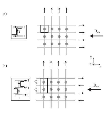
Figure 2: Basic configuration for the trapping of atoms in a periodic structure with 2 layers of wires. a) The currents in the layers are flowing in all wires in same direction. An additional bias field produces an array of Ioffe Pritchard type traps. The inset on the left side shows the unit cell in this lattice configuration (Configuration A). b) The currents in one layer are all flowing in the same direction, in the second layer the currents are bidirectional. With an additional bias field one gets an array of quadrupoles ($Q_{-}$,$Q_{+}$), which have different orientations of their quadrupole axis. The inset on the left side shows the unit cell in this lattice configuration (Configuration B).

Configuration A (currents in both layers unidirectional) has already been discussed in references Reichel2 ; Yin . We describe the concept using simple unit cells consisting of 3 wires segments crossing each other as marked in the box in fig. 2a. This unit cell has a central bar in the middle, enclosed by two wire segments in the upper and lower part of the unit cell. The size of the unit cell is given by the distance between the wires in each layer. The lattice is a simple square lattice. By applying an external bias field in the x-direction as indicated in fig. 2a each ”H” shaped unit cell contains a Ioffe Pritchard trap above the central bar. The basic properties of an individual trap can be calculated from the equations 5 and 6 given above for the ”Z”-trap plus a perturbation term, which will be calculated later.

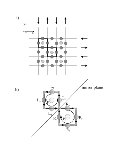
Figure 3: a) Lattice configuration with bidirectional currents in both layers. This gives a rich structure of quadrupoles in different directions. b) The simple unit cell for this array of wires consists of 6 wires. Without an external bias field this configuration yields 10 different quadrupoles as explained in the text (Configuration C).

In configuration B, the currents are unidirectional in one layer (y) and alternating in the second layer (x) (see fig 2 b). Here the simple unit cell consists of 4 wire segments as shown in fig. 2 b). The lattice is rectangular. By applying an external bias field in the x-direction two different quadrupole traps $Q_{-}$,$Q_{+}$, (see fig. 2b) are contained above the surface in the unit cell, which can be described by the equations 2 and 3 given for a quadrupole trap plus a perturbation term. The difference between the two quadrupoles in the unit cell is the orientation. At quadrupole $Q_{-}$ the axis is lying in the x,z plane under an angle of $-45^{\circ}$ with respect to the x-axis, and at quadrupole $Q_{+}$ the axis is under an angle of $45^{\circ}$ with respect to the x-axis. The quadrupoles can be used for magneto optical trapping to catch atoms in a reflection MOT Reichel2 ; Lee ; Schneble . Due to the fact that the two quadrupoles have different orientations, the circular polarisation of the MOT beams has to be different to either use the upper or the lower of the quadrupoles as will be shown in the experimental section.

In configuration C, the currents are alternating in both layers (fig. 3a). The unit cell consists of 8 wire segments. Even without an external bias field in this cell 10 different quadrupoles can be found. The bias field for all the different quadrupoles is given by the neighboring wires as mentioned before Thywissen , so no external bias field is necessary. Eight of the quadrupoles can be found above the wires ($R_{1}$..$R_{4}$ and $L_{1}$..${L_{4}}$, see fig. 3). The quadrupole axes of all of them are tilted by $45^{o}$ against the surface with respect to the wires and can be used for a reflection MOT Reichel2 ; Lee ; Schneble . Two other quadrupoles ($P_{1}$,$P_{2}$) are built up by two concentric wire squares Thywissen . The quadrupole axes of these two are oriented perpendicular to the surface, and thus they can not be used for a reflection MOT. The unit cell itself is symmetric under a mirror operation around the mirror plane as indicated in fig. 3 b). The lattice is a simple square lattice.

In all three configurations, the magnetic field $\vec{B}$ in the unit cell is given by the magnetic field produced by the wires in the unit cell $\vec{B}_{c}$ plus a perturbation term from the rest of the lattice $\vec{B}_{p}$

$$\vec{B}=\vec{B}_{c}+\vec{B}_{p}$$ (7)

For configuration A the perturbation in one cell can be expressed by the formula

$$\vec{B}_{p} = \frac{\mu_{0}I}{2\pi}\sum_{\begin{array}[]{c}n=-\infty\\ n\neq 0\end{array}}^{\infty}\frac{1}{(x-nd)^{2}+z^{2}}\cdot\left(\begin{array}[]{c}x-nd\\ 0\\ -z\end{array}\right)$$ (13)

$$+ \frac{\mu_{0}I}{2\pi}\sum_{\begin{array}[]{c}m=-\infty\\ m\neq 0\end{array}}^{\infty}\frac{1}{(y-md)^{2}+z^{2}}\cdot\left(\begin{array}[]{c}0\\ y-md\\ -z\end{array}\right)$$ (19)

and for configuration B

$$\vec{B}_{p} = \frac{\mu_{0}I}{2\pi}\sum_{\begin{array}[]{c}n=-\infty\\ n\neq 0\end{array}}^{\infty}\frac{(-1)^{n}}{(x-nd)^{2}+z^{2}}\cdot\left(\begin{array}[]{c}x-nd\\ 0\\ -z\end{array}\right)$$ (25)

$$+ \frac{\mu_{0}I}{2\pi}\sum_{\begin{array}[]{c}m=-\infty\\ m\neq 0\end{array}}^{\infty}\frac{1}{(y-md)^{2}+z^{2}}\cdot\left(\begin{array}[]{c}0\\ y-md\\ -z\end{array}\right)$$ (31)

where d is the distance between the wires and I the current flowing in the wires. The sums over n and m runs over all wires in the two horizontal directions. The terms for $n=m=0$ are excluded from the sum since only the perturbation from the rest of the lattice on a given unit cell should be considered here. An analogous situation is given in the third configuration. The perturbations to the magnetic field in one lattice cell will be small, if $d$ is much larger than the distance $z=r_{m}$ of the potential minimum from the surface.

For finite systems and $r_{m}\gg\ d$ the sum above is finite and one has to consider edge effects, which perturb the symmetry. This is analogous to finite-size magnetic mirrors used in atom optics Lau . The effect can be compensated by adding compensation wires, as proposed in Zabov .

III Experimental setup

To test the configurations proposed in section II.2 arrays of magnetic quadrupole traps are created by 2 layers of macroscopic wires mounted inside a vacuum chamber (see fig. 4). Each layer of wires consists of a ribbon UHV cable with a pitch of 1.27 mm (Caburn, Kapton Ribble Wire). The individual wires are kapton insulated with a diameter of the copper core of 0.25 mm. The cables are glued together with UHV compatible epoxy and are mounted on top of each other in a two layers configuration, where the upper layer consists of 10 wires in parallel and the lower layer consists of 8 parallel wires below the first one. The distance between the center of the wires in the two layers is 1.27 mm, given by the wire diameter. The whole wire assembly is attached to a Cu holder. The maximum current in the wires was about 5A. At higher currents, the pressure in the vacuum chamber started to increase probably due to outgasing of the insulating kapton layer. On top of the upper layer of wires a Si plate (thickness: 0.4 mm) covered with 10nm of Cr and 100 nm of Au is mounted, which serves as mirror. The whole setup is mounted upside down inside the chamber. The mirror at the surface is necessary, because we use the reflection MOT principle Reichel2 ; Lee ; Schneble to catch cold ${}^{87}Rb$ atoms. For this type of MOT two of the laser beams are parallel to the surface and two other lasers beams are reflected from the surface under an angle of $45^{\circ}$. The magnetic quadrupole field necessary for the MOT is generated by the two layers of wires plus an external bias field. This bias field can be adjusted between 0 G and 80 G. The circular polarisation of the four beams depends on the orientation of the magnetic quadrupole. The ${}^{87}Rb$ is provided by a Rb dispenser SAES ; Fortagh mounted approximately 4 cm away from the assembly. The optical access is provided by a large window below the sample.

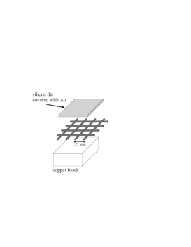
Figure 4: Experimental setup inside the vacuum chamber. Above a copper block 2 layers of kapton insulated wires are mounted under a gold covered silicon plate. The whole setup is mounted upside down inside the vacuum chamber.

To operate the MOT, we use as lasers two home built grating feedback stabilized diode lasers, operating at 780 nm. The cooling laser is locked on the $5S_{1/2},F=2\rightarrow 5P_{3/2},F^{\prime}=3$ cycling transition using polarisation spectroscopy in a vapor cell. The laser power in this laser is about 17 mW. The repumping laser is locked to the $5S_{1/2},F=1\rightarrow 5P_{3/2},F^{\prime}=2$ transition using the same locking scheme as for the MOT laser. This laser has a total power of 7 mW.

To detect the atoms in the MOT, we used a calibrated 8-bit CCD Camera, placed 8 cm under the surface outside the vacuum chamber. The imaging system is set up in a way, that atoms above the whole surface inside the chamber can be detected. One pixel on the camera corresponds to a $39\mu$m$\times$$36\mu m$ area in the trap region.

IV Experimental results

By using one wire in the upper one of the two layers together with the external bias field and turning on all the MOT beams one has the situation of a 2D MOT with additional optical molasses on the axis parallel to the surface (see fig. 5), upper left corner). This 2D-MOT can be extended to a 3D-MOT by using the wires of the lower layer transform the 2-D quadrupole to an 3-D quadrupole. In the experiments we used in the lower layer the two outermost wires of our experimental setup, which are at a distance of 10.1 mm (see fig. 5).

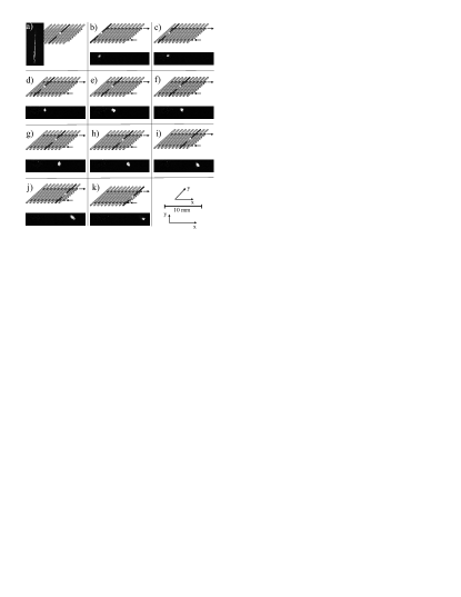
Figure 5: a) Two-dimensional MOT produced by the magnetic field of a single wire with a current of 4 A and an external bias field of 3 G. All MOT beams are turned on yielding a 2-D MOT with an optical molasses on the y-axis. b-k): MOTs with a magnetic quadrupole field produced by two layers of wires. By turning on the current in two wires in the x-direction MOTs at different position above the surface can be addressed by using different wires. The wires used are indicated above the images. The currents in the wires were 4 A with an external bias field of 3 G. The distance between the wires in the x-direction is 1.27 mm (left to right in the picture), the distance between the current-carrying wires in the y-direction is 10.2 mm.

We found that the position of the MOT can be precisely controlled by choosing the current carrying wire in the upper layer. The currents were set to 4 A and an external bias field of 3 G was applied. With these values the magnetic field gradients be calculated from equations 2 and 3 as $\frac{dB}{dx}=11G/cm$ and $\frac{dB}{dy}=1.9G/cm$. The calculated distance $r_{m}$ from the MOT to the surface is 1.6 mm.

In this configuration, a MOT was realized above every wire (see fig. 5). The average number of atoms for the different MOT positions was $3\cdot 10^{5}$. A situation where no external bias field was necessary was reached by using as bias field wires the neighboring wires on the left and on the right of the MOT wire in the upper layer with current flowing in the opposite direction. The number of atoms in such a MOT generated without external field was lower, due to the fact that the capture range was smaller. The reason for this is the fact that the bias field produced by the two neighboring wires is inhomogeneous. The quadrupoles resulting from this configuration extend over a smaller volume and so the capture range is reduced.

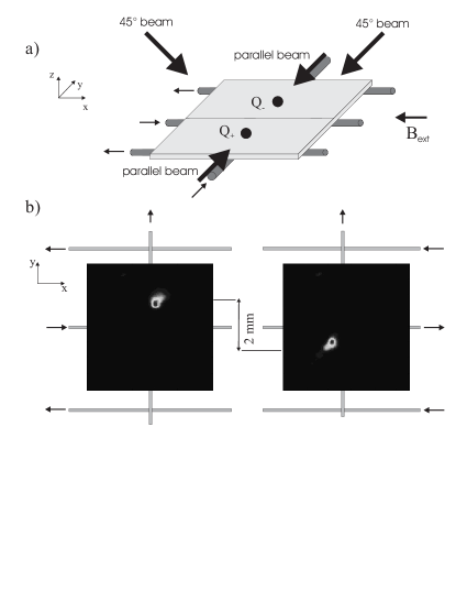
Figure 6: a) Experimental realization of the unit cell of configuration B. The wire configuration is consists of 4 wire segments. In the reflection-MOT configuration 2 MOT beams are reflected from the surface and 2 beams are parallel to the surface (arrows). b) Switching between the different MOTs by changing the circular polarisation of the beam parallel to the surface. The current in the wires was 4 A, the external bias field 3 G. The position displacement by changing the polarisation is about 2 mm in the y-direction and 0.2 mm in the x-direction. The change in position in x-direction is probably due to an imbalance in the MOT beams.

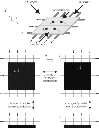
Figure 7: a) Experimental realization of the unit cell of configuration C. The wire configuration consists of 7 wires, of which for the experiments only 6 are used simultaneously. In the MOT configuration 2 MOT beams are reflected from the surface and 2 beams are parallel to the surface (arrows). b,c)-d,e) switching between the different MOTs by reversing the circular polarisation of the beams parallel to the surface. b,d)-c,e) switching between the MOTs by reversing the circular polarisation of the $45^{\circ}$ MOT beams. The current in the wires was 4 A, the external bias field 3 G.

In the proposed configuration B two quadrupoles which are different in orientation emerge above the middle wire segment of the unit cell. These two quadrupoles can be used to operate the MOT, if the respective polarisations of the MOT laser beams fit to the orientation of the quadrupoles. In our experimental setup, we realized the unit cell configuration consisting of 4 wires (see fig. 6a). The distance between the parallel wires was 5mm (upper - middle wire), respectively 3.8 mm (middle - lower wire). The current in each of the wires was chosen as 4 A and an external bias field of 3 G was applied. This yields a gradient of $\frac{dB}{dx}=11G/cm$ in the x- and $\frac{dB}{dy}=3.3G/cm$ in the y-direction. The distance $r_{m}$ above the surface is again $1.6mm$. By changing the polarisation of the MOT beams parallel to the surface from $\sigma^{+}$ to $\sigma^{-}$ the MOT changes its position due to the two different orientations of the two quadrupoles within the rectangular unit cell (see fig. 6 b).

In configuration C, 10 quadrupoles are created per unit cell without external fields. As explained before 8 of these quadrupoles are in principle suited to operate a reflection MOT, because the angle between the quadrupole axis and surface is $45^{\circ}$. In our experimental configuration only four of them can be seen due to the fact that only for four quadrupoles the axes coincide with the direction of a MOT beam. The accessible positions can again be addressed by changing the polarisation of the MOT beams, where the polarisation configuration is determined by the orientation of the magnetic quadrupoles for the different wire configurations (see fig. 7a). For the generation of the magnetic field in the unit cell we used 3 wires in the y-direction with alternating currents (distance wire-wire 2.5mm) and 3 wires in the x-direction (distance between the wires 5 mm, respectively 3.8 mm, as in configuration B). By building up only one such lattice cell, the quadrupoles at the edges of the lattice cells are not accessible, because only in the middle of the cell the bias field needed is produced by the neighboring wires. So we investigated in this configuration the quadrupoles in the middle of the unit cell ($R_{2}$,$L_{4}$). Then we switched off the current in the left wire, and turned on the current in the right wire to be able to observe the quadrupoles $R_{4}$ and $L_{2}$ (see configuration marked in fig. 7b-e). To reach a stable situation the current in the two middle wires was in both cases 3.5 A (y-direction) and in the outermost wires 5A. These values yield a distance of the quadrupole from the surface of 0.2 mm and a gradient $\frac{dB}{dx}=20G/cm$ in the x-direction. The currents in the x direction were 4A. This yields a gradient of $\frac{dB}{dy}=9.7G/cm$ in the y-direction. As shown in fig. 7b-e the different quadrupoles can be addressed by changing the polarisations of the MOT beams as expected. By changing the circular polarisation of the beams parallel to the surface we can switch between $L_{4}$ and $R_{2}$ (see fig. 7b,c) and $L_{2}$ and $R_{4}$ (see. fig. 7d,e) respectively. The distance change in the y-direction is 4.4 mm respectively 4 mm and in the x-direction 1 mm. By changing the circular polarisation of the $45^{\circ}$ beams (see fig. 7b,d, c,e) one can switch between $L_{4}$ and $L_{2}$, respectively between $R_{2}$ and $R_{4}$. Here the observed change in position in x direction is 2.2 mm. The number of atoms in the different MOTs is between $8\cdot 10^{4}$ and $2.4\cdot 10^{5}$ atoms. The main advantage of this configuration compared to configuration B is the fact that no external bias field in necessary.

Figure 8: a) Current distribution in the lattice to observe an 2x2 array of MOTs. In the y-direction 2 wires are used as indicated in the picture. In the x-direction two neighboring wires are used as one effective wire. b) 2x2 array of MOTs above the surface. By using 2 wires in the y and 4 effective wires in the x-direction a stable situation with 4 MOTs above the surface can be generated. The number of atoms in each individual MOT is about $2\cdot 10^{5}$ atoms. The distance between the different MOTs is 3.3 mm in the y- and 8 mm in the x-direction. c,d) By applying an additional laser beam to the positions of the MOTs these can be individually turned on and off by blowing the cold atoms away.

Up to now only single unit cells were observed. To built up lattices it is necessary to create arrays of unit cells. This can be done in the experiment by using more wires. For an array of MOTs, we arranged 4 unit cells in configuration B. As explained before it is necessary that the distance between the wires has to be large compared to the distance of the field minimum $r_{m}$ to the wire. To reach this, we used two wires in the x-direction with a distance of 10.16 mm from each other. In the y-direction we used two wires in pairs (current flowing in the same direction) as one effective wire with a current of about 3 A in each of the effective wires (see fig. 8a). The complete configuration in this direction is given by 4 of these wire pairs. The current in the wires of the upper layer was also 3 A, the bias field was 4 G. With this configuration, we could generate a stable situation with 4 MOTs operating above the surface (see fig. 8b). The gradient of the quadrupole in the x-direction is again $\frac{dB}{dx}=20G/cm$ and in the y-direction $\frac{dB}{dy}=4.3G/cm$. The calculated distance $r_{m}$ above the surface is about $1$ mm. The number of atoms in each individual MOT is about $2\cdot 10^{5}$. The distance between the different MOTs is 3.3 mm in the x- and 8 mm in the y-direction. To switch the MOTs individually, we applied a laser pulse split off from the MOT laser to turn the different MOTs on and off by blowing the atoms away (see fig. 8c,d). By turning off one MOT no significant change in atom number of the remaining MOTs could be detected.

V Summary

In this paper, we have proposed different lattice configurations consisting of magnetic quadrupoles which are generated by 2 orthogonal layers of wires. These quadrupoles could be detected in the different unit cells by operating MOTs with the required polarisation configuration. We could furthermore demonstrate the possibility to use this two layer configuration to trap atoms in a 2x2 MOT array above a surface. We were able to turn the MOTs on and off individually by using an extra laser beam. Such a system of multiple MOTs could be useful to load an array of magnetic microtraps from an array of separate MOTs. The current number of $10^{5}$ atoms in the single MOT will be increased in future experiments by using the Rb dispenser in our chamber in a pulsed operation with higher currents.

References

- (1) J.D. Weinstein and K.G. Libbrecht, Phys. Rev. A52, 4004 (1995).
- (2) J. Reichel, W. Hänsel and T.W. Hänsch, Phys. Rev. Lett. 83, 3398 (1999).
- (3) W. Hänsel, J. Reichel, P. Hommelhoff and T. W. Hänsch, Phys. Rev. Lett. 86, 608 (2001).
- (4) D. Cassettari, B. Hessmo, R. Folman, T. Maier and J. Schmiedmayer, Phys. Rev. Lett. 85, 5483 (2000).
- (5) H. Ott, J. Fortagh, G. Schlotterbeck, A. Grossmann and C. Zimmermann, Phys. Rev. Lett. 87, 230401 (2001).
- (6) W. Hänsel, P. Hommelhoff, T. W. Hänsch and J. Reichel, Nature 413, 498 (2001).
- (7) R. Folman, P. Krüger, J. Denschlag, C. Henkel and J. Schmiedmayer, Adv. At. Mol. Opt. Phys. 48, 263 (2002).
- (8) J. Reichel, Appl. Phys. B75, 469 (2002).
- (9) R. Frisch and E.Segrè, Z. Phys. 80, 610 (1933).
- (10) A. Haase, D. Cassettari, B. Hessmo and J. Schmiedmayer, Phys. Rev. A64, 043405 (2001).
- (11) J.H. Thywissen, M. Olsanii, G. Zabow, M. Drndić, K.S. Johnson, R.M. Westerwelt and M. Prentiss , Eur. Phys. J. D7, 361 (1999).
- (12) J. Reichel, W. Hänsel, P. Hommelhoff and T.W. Hänsch:, Appl. Phys. B72, 81 (2001).
- (13) J. Yin, W. Gao, J. Hu and Y. Wang, Opt. Commun. 206, 99 (2002).
- (14) E. A. Hinds, C. J. Vale and M. G. Boshier, Phys. Rev. Lett. 86, 1462 (2001).
- (15) D.C. Lau, A.I. Sidorov, G.I. Opat, R.J. McLean, W.J. Rowlands and P. Hannaford, Eur. Phys. J. D5, 193 (1999).
- (16) K. I. Lee, J. A. Kim, H. R. Noh and W. Jhe, Opt. Lett. 21, 1177 (1996).
- (17) D. Schneble, H. Gauck, M. Hartl, T. Pfau and J. Mlynek, in Proceedings of the International School of Physics ”Enrico Fermi” Course CXL, edited by M. Inguscio, S. Stringari, and C.E. Wieman (IOS Press Amsterdam, 1999), pp. 469-490.
- (18) G. Zabow, M. Drndić, J.H. Thywissen, K.S. Johnson, R.M. Westervelt and M. Prentiss, Eur. Phys. J. D7, 351 (1999).
- (19) SAES Getters S.p.A., 20151 Milano, Italy.
- (20) J. Fortagh, A. Grossmann, T. W. Hänsch and C. Zimmermann, J. Appl. Phys. 84, 6499 (1998).