Total suppression of a large spin tunneling barrier in quantum adiabatic computation

Abstract

We apply a quantum adiabatic evolution algorithm to a combinatorial optimization problem where the cost function depends entirely on the of the number of unit bits in a $n$-bit string (Hamming weight). The solution of the optimization problem is encoded as a ground state of the problem Hamiltonian $H_{p}$ for the $z$-projection of a total spin-$\frac{n}{2}$. We show that tunneling barriers for the total spin can be completely suppressed during the algorithm if the initial Hamiltonian has its ground state extended in the space of the $z$-projections of the spin. This suppression takes place even if the cost function has deep and well separated local minima. We provide an intuitive picture for this effect and show that it guarantees the polynomial complexity of the algorithm in a very broad class of cost functions. We suggest a simple example of the Hamiltonian for the adiabatic evolution: $H(\tau)=(1-\tau)\,\hat{S}_{x}^{2}+\tau\,H_{p}$, with parameter $\tau$ slowly varying in time between $0$ and $1$. We use WKB analysis for the large spin to estimate the minimum energy gap between the two lowest adiabatic eigenvalues of $H(\tau)$.

I Introduction

Recently a novel paradigm was suggested for the design of quantum algorithms for solving combinatorial search and optimization problems based on quantum adiabatic evolution Farhi . In the quantum adiabatic evolution algorithm (QAA) a quantum state closely follows a ground state of a specially designed slowly varying in time control Hamiltonian. At the initial moment of time the control Hamiltonian has a simple form with the known ground state that is easy to prepare; at the final moment of time it coincides with the “problem” Hamiltonian $H_{P}$ whose ground state encodes the solution of the classical optimization problem in question. It can also be chosen to reflect the bit-structure and cost spectrum of the problem. For example,

$$H_{P}=\sum_{\bf z}E_{\bf z}|{\bf z}\rangle\langle{\bf z}|$$ (1)

$$|{\bf z}\rangle=|z_{1}\rangle_{1}\,\otimes|z_{2}\rangle_{2}\,\otimes\cdots\otimes|z_{n}\rangle_{n}.$$

Here $E_{\bf z}$ is a cost function defined on a set of $2^{n}$ binary strings ${\bf z}=\{z_{1},\ldots,z_{n}\}$ $z_{j}=0,1$, each containing $n$ bits. The summation in (1) is over $2^{n}$ states $|{\bf z}\rangle$ forming the computational basis of a quantum computer with $n$ qubits. State $|z_{j}\rangle_{j}$ of the $j$-th qubit is an eigenstate of the Pauli matrix $\hat{\sigma}_{z}$ with eigenvalue $1-2z_{j}=\pm 1)$. If at the end of the QAA the quantum state is sufficiently close to the ground state of $H_{P}$ then the solution to the optimization problem can be retrieved by measurement.

Running of the algorithm for several NP-complete problems has been simulated on a classical computer using a large number of randomly generated problem instances that are believed to be computationally hard for classical algorithms FarhiSc ; FarhiSat ; FarhiCli . Results of these numerical simulations for relatively small size of the problem instances ( $n\leq$ 20) suggest a quadratic scaling law of the run time of the quantum adiabatic algorithm with $n$. Furthermore, it was shown in Vazirani02 that the previous query complexity argument that lead to the exponential lower bound for unstructured search Bennett cannot be used to rule out the polynomial time solution of NP-complete Satisfiability problem by QAA.

On the other hand, a set of examples of the 3-Satisfiability problem has been recently constructed Vazirani01 ; annealing ; Vazirani02 to test analytically the power of QAA in the situations where the optimization problem in question has multiple well-separated local minima.

In these examples the cost function $E_{\bf z}$ depends on a bit-string ${\bf z}$ with $n$ bits, ${\bf z}=\{z_{1},z_{2},\ldots,z_{n}\}$, only via the Hamming weight of the string, $w_{\bf z}=(z_{1}+z_{2}+\ldots+z_{n})$, so that $E_{\bf z}=f\left(w_{\bf z}\right)$. The function $f(w)$ is multi-modal, it has a local minimum separated from the global minimum by the barrier of an order-$n$ width in $w$. For that reason classical local search like simulating annealing provably fails to find a globally optimal solution in time polynomial in $n$. It annealing ; Vazirani02 a “standard” QAA was applied to this problem in which a quantum evolution begins in a uniform superposition state $\frac{1}{\sqrt{2^{n}}}\sum_{\bf z}|{\bf z}\rangle$, ends in a target (solution) state $|{\bf z}_{t}\rangle$, and the control Hamiltonian is a linear interpolation in time between the initial and final Hamiltonians.

For the above examples it was shown annealing ; Vazirani02 that the system can be trapped during the QAA in the local minimum of a cost function for a time that grows exponentially in the problem size $n$. It was also shown annealing that an exponential delay time in QAA can be computed in terms of a quantum-mechanical tunneling for an auxiliary large spin system.

It can also be inferred from Vazirani02 ; annealing that QAA will have an exponential complexity even if the cost function $E_{\bf z}$ no longer depends strictly on a Hamming weight but the deviation only occurs for states $|{\bf z}\rangle$ that have exponentially small (in $n$) overlap with the adiabatic ground state wavefunction $|\phi_{0}(t)\rangle$ at all times during the algorithm execution.

The above example has a significance more than just being a particular simplified case of the binary optimization problem with symmetized cost. Indeed one can argue that it shows one of the mechanisms for setting “locality traps” in the 3-Satisfiability problem Vazirani_talk . But most importantly, this example demonstrates that exponential complexity of QAA results from a collective phenomenon in which transitions between the bit-configurations with low-lying energies can only occur by the simultaneous flipping of large clusters containing order-n bits. In many cases these transitions can be analyzed as a tunneling of spin variables. A similar phenomenon related to the tunneling of magnetization was recently observed in the large-spin molecular nanomagnets Wernsdorfer .

However low-energy collective behavior is also well known in spin glass models, many of which are in one-to-one correspondence with random NP-complete problems Anderson . In particular, an important ingredient of the “replica symmetry breaking” picture of an infinite-range spin glass by Parizi Parizi is that there are collective spin exitations that are of the order of the system size $n$ whose energy is $({\cal O}(1)$, i.e., it does not grow with the size of the system. A similar picture may be applicable to random Satisfiability problems Monasson .

Therefore in connection to the above example, it is important to understand how to design a polynomial time QAA without a prior knowledge of a particular form of the cost function $f\left(w\right)$ (possibly multi-modal or even randomly sampled), so that a tunneling barrier between the local minima will be totally suppressed. This is a focus of the present paper footnote1 .

In Sec. III we present a theory of quantum adiabatic evolution of a large spin system introducing a control Hamiltonian that guarantees polynomial time complexity for QAA in the symmetrized 3-Satisfiability example mentioned. In Sec. IV we provide an estimate of the minimum gap between the two lowest eigenvalues of the control Hamiltonian that determines the complexity of QAA. Sec. V contains concluding remarks.

II Quantum Adiabatic Evolution Algorithm

In a standard QAA Farhi one specifies the time-dependent Hamiltonian $H(t)=\tilde{H}(t/T)$

$$\tilde{H}(\tau)=(1-\tau)\,H_{D}+\tau\,H_{P},$$ (2)

where $\tau=t/T$ is dimensionless “time”. This Hamiltonian guides the quantum evolution of the state vector $|\psi(t)\rangle$ according to the Schrödinger equation $i\,{\partial|\psi(t)\rangle\partial t}=H(t)|\psi(t)\rangle$ from $t=0$ to $t=T$, the run time of the algorithm (we let $\hbar=1$). $H_{P}$ is the “problem” Hamiltonian given in (1). $H_{D}$ is a “driver” Hamiltonian, that is designed to cause the transitions between the eigenstates of $H_{P}$. In this algorithm one prepares the initial state of the system $|\psi(0)\rangle$ to be a ground state of $\tilde{H}(0)=H_{D}$. It is typically constructed assuming ${\it no}$ knowledge of the solution of the classical optimization problem and related ground state of $H_{P}$. In the simplest case

$$H_{D}=-C\,\sum_{j=0}^{n-1}\hat{\sigma}_{x}^{j},\quad|\psi(0)\rangle=2^{-n/2}\sum_{\bf z}|{\bf z}\rangle,$$ (3)

where $\sigma_{x}^{j}$ is a Pauli matrix for $j$-th qubit and $C>0$ is some scaling constant. Consider instantaneous eigenstates $|\phi_{k}(\tau)\rangle$ of $\tilde{H}(\tau)$ with energies $E_{k}(\tau)$ arranged in nondecreasing order at any value of $\tau\in(0,1)$

$$\tilde{H}|\phi_{k}\rangle=E_{k}|\phi_{k}\rangle,\quad k=0,1,\ldots,2^{n}-1.$$ (4)

Provided the value of $T$ is large enough and there is a finite gap for all $t\in(0,T)$ between the ground and exited state energies, $\Delta E(\tau)=E_{1}(\tau)-E_{0}(\tau)>0$, quantum evolution is adiabatic and the state of the system $|\psi(t)\rangle$ stays close to an instantaneous ground state, $|\phi_{0}(t/T)\rangle$ (up to a phase factor). Because $H(T)=H_{P}$ the final state $|\psi(T)\rangle$ is close to the ground state $|\phi_{0}(\tau=1)\rangle$ of the problem Hamiltonian. Therefore a measurement performed on the quantum computer at $t=T\,(\tau=1)$ will find one of the solutions of combinatorial optimization problem with large probability. Quantum transition away from the adiabatic ground state occurs most likely in the vicinity of the point $\tau\approx\tau_{c}$ where the energy gap $\Delta E(\tau)$ reaches its minimum (avoided-crossing region). The probability of the transition, $1-|\langle\psi(t)|\phi_{0}(t/T)\rangle|^{2}_{t=T}$, is small provided that

$$T\gg\frac{|\langle\phi_{1}|\tilde{H}_{\tau}|\phi_{0}\rangle|_{\tau=\tau_{c}}}{\Delta E_{\rm min}^{2}},\quad\Delta E_{\rm min}=\min_{0\leq\tau\leq 1}\left[E_{1}(\tau)-E_{0}(\tau)\right],$$ (5)

($\tilde{H}_{\tau}\equiv d\tilde{H}/d\tau$). The fraction in (5) gives an estimate for the required runtime of the algorithm and the task is to find its asymptotic behavior in the limit of large $n\gg 1$. The numerator in (5) is less than the largest eigenvalue of $\tilde{H}_{\tau}=H_{P}-H_{D}$, typically polynomial in $n$ Farhi . However, $\Delta E_{\rm min}$ can scale down exponentially with $n$ and in such cases the runtime of quantum adiabatic algorithm will grow exponentially fast with the size of the input $n$.

II.1 Binary optimization problems with symmetrized cost function

Consider a cost function $E_{\bf z}$ in the following form:

$$E_{\bf z}=f\left(w_{\bf z}\right),\quad w_{\bf z}=\sum_{j=1}^{n}z_{j}.$$ (6)

This cost is symmetric with respect to the permutation of bits and $w_{\bf z}$ is a Hamming weight of a string ${\bf z}$. A particular example of this problem related to 3-Satisfiability was introduced in Vazirani01 ; annealing ; Vazirani02 (the discussion in this subsection closely follows annealing , Sec. 4). In this example

$$E_{\bf z}=\sum_{i<j<k}c(z_{i}+z_{j}+z_{k}),$$

$$c(m)=(1-\delta_{m,0})\,\left(1+\delta_{m,1}(q-1)\right),\quad m=0,1,2,3$$ (7)

where $\delta_{k,l}$ is a Kronecker delta. For this particular case function $f(w)$ in (6) takes the following form:

$$f(w)=\frac{q}{2}w(n-w)(n-w-1)+\frac{1}{2}w(w-1)(n-w)+\frac{1}{6}w(w-1)(w-2).$$ (8)

where $q$ is an integer greater than or equal to 3. In the leading order in $n\gg 1$ one can write:

$$f(w)=\left(\frac{n}{3}\right)^{3}\,g\left(\frac{w}{n}\right)+{\cal O}(n^{2}),$$ (9)

where

$$h(u)=4qu(1-u)^{2}+4u^{2}(1-u)+\frac{4}{3}u^{3}.$$ (10)

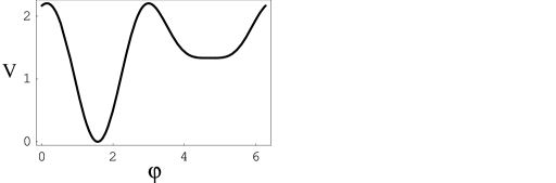
Figure 1: Multistable effective potential $V$ vs polar angle $\varphi$ for $q=3$.

$g(u)$ is a non-monotonic function with global minimum at $u=0$ corresponding to $z_{1},z_{2},\ldots,z_{n}=0$. It also has a local minimum at $u=1$ corresponding to $z_{1},z_{2},\ldots,z_{n}=1$ ( cf. Ref. annealing , Fig. 1).

In QAA the symmetrized cost function (8) corresponds to the following problem Hamiltonian $H_{P}$ of total spin-$n/2$ system (cf. Eq. (1) )

$$H_{P}=f\left(\frac{n}{2}-\hat{S}_{z}\right),$$ (11)

where

$$\hat{S}_{z}|{\bf z}\rangle=S_{z})|{\bf z}\rangle,\quad S_{z}=\frac{n}{2}-w_{\bf z}.$$ (12)

Here $\hat{S}_{z}$ is operator of $z$-projection of a total spin $\frac{n}{2}$ of a system of $n$ individual spins $1/2$. We used an obvious connection between the values of the Hamming weight function $w_{\bf z}$ and corresponding eigenvalues $S_{z}$ of the operator $\hat{S}_{z}$. In what following we use “hat” notation for the operators of a total spin.

It was shown annealing that if one uses $H_{D}$ in a form corresponding to (3)

$$H_{D}=\binom{n-1}{2}\left(\frac{n}{2}-\hat{S}_{x}\right).$$ (13)

then the minimum gap $\Delta E_{\rm min}$ scales down exponentially with $n$ implying the exponential complexity of QAA for this problem.

III Adiabatic Evolution of a Large Spin

III.1 Extended vs localized initial states

In this paper we show that the main reason for the exponentially small minimum gap for the problem (7) with $H_{D}$ given in (13) is the fact that the ground state of the driving Hamiltonian is localized in the space of the $z$-projections of a total spin. We construct an example of the driving Hamiltonian with extended ground state and show that in this case the evolution time of QAA is polynomial in the number of qubits.

In the following we adopt the notation for the total spin $\hat{\bf S}=\left\{\hat{S}_{j}\right\}$, with $j=x,y,z$, where $\hat{S}_{j}$ are the projections of the total spin operator on the $j$-th axis. The total spin operator’s components equal $\hat{S}_{j}=\sum_{k=1}^{n}\hat{S}_{j}^{\left(k\right)}$ and are symmetric in all one-qubit spin operators $\left\{\hat{S}_{j}^{\left(k\right)}\right\}$ for $k=1,...n$. We use $S_{j}$ for the eigenvalues of the operator $\hat{S}_{j}$.

We now introduce a new driver Hamiltonian

$$H_{D}=\hat{S}_{x}^{2}.$$ (14)

Consider, for example, its ground state in the case when the total number of qubits $n=2s$ is even and therefore the total spin $l=n/2=s$ is an integer. Then the ground state is a state with $S_{x}=0$ in a basis where $x$ is chosen as a quantization axis. Making use of Wigner’s rotation matrix $d_{m,m^{\prime}}^{l}\left(\theta\right)$ LANDAU1 , one easily projects this state onto the computational (problem) basis with the $z$ quantization axis and $m=S_{z}$. This gives us the ground state wave function in the problem basis as $\Psi_{0}\left(m\right)=d_{m,0}^{l}\left(\pi/2\right)$. In the limit of large spin (which is the case of interest for us), the wave function is given by

$$\Psi_{0}\left(m\right)\approx\frac{\left(-1\right)^{k}}{\sqrt{2\pi}}\frac{1}{\left(l^{2}-m^{2}\right)^{1/4}}\delta_{l-m,2k},\qquad l=\frac{n}{2}\quad(n\,\,{\rm is\,\,even}).$$ (15)

Note that $\Psi_{0}\left(m\right)=0$ for the odd difference $l-m=2k+1$ and is given by (15) for $l-m=2k$. From (15), it follows that the ground state of $S_{x}^{2}$ is delocalized in the $m$- space and spread over the whole interval, $-l\leq m\leq l$.

On the other hand, the ground state of the operator (13) used in annealing as a driver, is localized in the $m$-space. Indeed, that ground state is a state with $S_{x}=l$ in the $x$ basis. This gives us the ground state wave function in the problem basis, $\Psi^{\prime}_{0}\left(m\right)=d_{m,l}^{l}\left(\pi/2\right)$. In the limit of large spin one has

$$\Psi^{\prime}_{0}\left(m\right)\approx\frac{1}{\sqrt{\pi l}}\exp\left(-\frac{m^{2}}{l}\right),$$ (16)

which is clearly localized on the scale $m^{2}\simeq l$. The same conclusion holds for the case when $n$ is odd and $l$ take half-integer values.

As we will show below, the adiabatic evolution of the delocalized states is fundamentally different from the localized ones. In particular, the localized ground states in general result in macroscopic tunneling. This gives the exponentially small in $n$ ground state energy gaps and consequently the exponentially large complexity of QAA. Using the delocalized states one can avoid macroscopic tunneling. We argue that in a general situation when the information about the ground state is not used for constructing the driver Hamiltonian, the driver with extended ground state should lead to polynomial complexity of adiabatic algorithms independently of the specific form of the problem Hamiltonian provided that it is expressed as a function (in general, nonlinear) of the total spin operators, $\hat{S}_{j}$ (cf. Eq. (11)).

III.2 WKB approximation for the large spin

To be specific, we refer to the same problem Hamiltonian as in Eq. (11). The full Hamiltonian takes the following form in the limit of large $n$

$$H\left(\tau\right)=\left(1-\tau\right)n\hat{S}_{x}^{2}+\tau\left(\frac{n}{2}\right)^{3}h\left(\hat{u}\right),$$ (17)

$$\hat{u}=\frac{1}{2}\left(1-\frac{\hat{S}_{z}}{l}\right),\qquad l=\frac{n}{2},$$

where $\tau=t/T$ ; $0\leq\tau\leq 1$ and function $h(u)$ is given in (10).

In order to get a simple physical picture, we will refer to the WKB-type approach commonly used in the theory of quantum spin tunneling in magnetics (QTM) CHUD1 , GARG1 , GARG2 . This approach is applicable for large spins $(l>>1)$, which is the case of interest for us. We choose $x$ as a quantization axis and following the standard procedure obtain the effective quasi-classical Hamiltonian in polar coordinates $\left\{\theta,\varphi\right\}$ with $\theta\in\left[0,\pi\right]$ and $\varphi\in\left[0,2\pi\right]$. In doing this, we make use of the following relations valid in the limit $(l>>1)$

$$S_{z}^{n}\approx\left(l\sin\theta\sin\varphi\right)^{n}.$$

As it was shown in GARG2 , in the quasi-classical limit we have

$$\hat{S}_{x}^{2}\approx-\frac{\partial^{2}}{\partial\varphi^{2}}\equiv\hat{p}^{2},\quad\theta\approx\frac{\pi}{2},$$ (18)

which means that the motion of the quasi-classical spin can be described as a 1D motion of a massive particle on a unit radius ring in the appropriate effective potential $V(\phi)$. We also have

$$u=\frac{1}{2}\left(1-\sin\varphi\right).$$ (19)

Substituting this into (17), we finally obtain the effective quasi-classical Hamiltonian in the form

$$H\left(\tau\right)=n\left(1-\tau\right)\hat{p}^{2}+\tau\left(\frac{n}{2}\right)^{3}\,V(\varphi),$$

$$\quad V(\varphi)=h\left(\frac{1-\sin\varphi}{2}\right).$$ (20)

One should note that the driver $H_{D}=n\hat{S}_{x}^{2}$ does not change the effective potential caused by $H_{P}$ and only introduces the effective kinetic energy into the problem. As we show below, this driver has extended eigenstates in the space of the $z$-projections $m$ of a total spin, as opposed to the case $H_{D}=n^{2}S_{x}$ considered in annealing , where the eigenstates are localized in $m$. As we will see below, this leads to the absence of tunneling and polynomial gap in our case as opposed to the exponentially small tunneling amplitude arising in annealing . The adiabatic wave functions $\Psi_{k}\left(\varphi\right)$ satisfy

$$\left[-\left(1-\tau\right)\frac{\partial}{\partial\varphi^{2}}+\tau\frac{n^{2}}{8}\,V(\varphi)\right]\Psi_{k}\left(\varphi\right)=\widetilde{E}_{k}\left(\tau\right)\Psi_{k}\left(\varphi\right),$$ (21)

where $\widetilde{E}_{k}\left(\tau\right)=E_{k}\left(\tau\right)/n$ is a rescaled energy. The first term in the l.h.s. of (21) corresponds to the driving Hamiltonian $H_{D}$ and presents the kinetic energy of the particle moving in the effective potential due to the problem Hamiltonian $H_{P}.$ At initial moment $\tau=0$, the total Hamiltonian reduces to the driver $H_{D}$ which describes a free massive particle on a ring and its eigenstates are well known LANDAU1 . In this case, the Schrödinger equation (21) gives exact wavefunctions and spectrum. Namely, we have

$$\Psi_{k}\left(\varphi\right) = \frac{1}{\sqrt{2\pi}}\exp\left(ik\varphi\right),$$ (22)

$$\widetilde{E}_{k}\left(0\right) = k^{2},$$

where $k$ is an integer number $k=0,\pm 1,\pm 2,...$ for even $n$ when the total spin $l=n/2$ is integer, and a half-integer number $k=\pm 1/2,\pm 3/2,...$ for an odd number of qubits $n$, when $l=[n/2]+1/2$. One should note that in case of integer spin $l$ , all eigenstates are twofold degenerate except for the ground state corresponding to $k=0$ and for the half-integer spin, all states including the ground state are twofold degenerate. This is a particular case of the Kramers’ degeneracy LANDAU1 , GARG1 , which occurs due to the symmetry with respect to the spin-flip transformation. Note that since from (19) it follows that $m=l\sin\varphi$, the states (22) are indeed delocalized in the $m$-space.

From (21), it follows that the problem Hamiltonian is of the same order of magnitude as the driving one only for sufficiently short times $\tau n^{2}\simeq 1$. This means that the problem Hamiltonian is of the order of the level separation of the kinetic term only for sufficiently small times. Since the eigenstates of the driving Hamiltonian are extended (delocalized) in $m$, this implies the following qualitative picture of adiabatic evolution of the ground energy level with $\tau$ . At sufficiently small times $\tau n^{2}\ll 1$, the term due to $H_{P}$ can be considered as a perturbation to the driver term and the energy levels are not strongly distorted. The eigenstates are delocalized in the $m$ space. As $\tau$ increases, the ground state is affected by the perturbation and the ground state energy increases.

III.3 Minimum gap analysis

If the ground state is not degenerate (this is the case when the total number of qubits $n=2s$ is even), the gap may have a non-monotonic behavior in $\tau$ in the range $\tau n^{2}\simeq 1$. Qualitatively, this can be described as follows. For sufficiently small times $\tau n^{2}\ll 1$, the ground state energy is increasing in $\tau$ due to the diagonal matrix elements of the problem Hamiltonian until compensated by the level repulsion from the first excited state. After this, the ground state is pushed down and gradually approaches the ground state of $H_{P}$ (which is $E_{g}=0$ in the present case). Since the upper levels are not as strongly affected by the perturbation as the ground state and since the number of upper levels is very large, ${\cal O}(n)$, the system of upper levels behaves as a rigid one. For this reason the strong interaction between the ground and first excited states occurs in the range of energies $\Delta E$ corresponding to the the level separation in the driver Hamiltonian and is linear in $n$. Therefore

$$\Delta E={\cal O}\left(n^{-2}\Delta E_{P}\right),$$ (23)

where $\Delta E_{P}$ denotes the separation between the two lowest eigenvalues of $H_{P}$. Clearly, the energy scale of the minimal gap is polynomial in the number of qubits $n$ provided that $\Delta E_{P}$ is polynomial.

As we have discussed above, in case of an odd number of qubits, all initial eigenstates of $H_{D}$ have a twofold degeneracy (Kramers’ degeneracy). In this case, the degeneracy is removed by the effective potential (Zeeman splitting) and there is no avoided-crossing between the ground state and the first excited states of the total Hamiltonian $H(\tau)$. One can easily show that in this case the level separation $E_{1}(\tau)-E_{0}(\tau)$ grows monotonically in $\tau$ LANDAU1 (it is linear in $\eta$ for $\eta\ll 1$).

Apart from the features occurring in the range of small $\tau\simeq n^{-2}$, the evolution of the ground state on the large time scale $\tau\simeq 1$ is the same for both even and odd number of qubits. Most importantly, the estimate (23) holds globally in both cases. As we will see below, this is confirmed by numerical simulations.

IV Minimal Gap Estimate

As we discussed above, the ground state energy may have a non-monotonic time dependence on $\tau$ when the total number of qubits is even and the ground state of $H_{D}$ is not degenerate. Because the eigenvalues of the driver Hamiltonian, $n\,k^{2}$, grow rapidly with the quantum number $k$ it is possible to obtain a minimum gap estimate analyzing how $H_{P}$ affects the two lowest eigenvalues of the driver. Making use of (2), we obtain the adiabatic gap as a function of time in the range $\tau n^{2}\lesssim 1$

$$E_{1}(\tau)-E_{0}(\tau)\approx\sqrt{\left[\left(1-\tau\right)n-\tau\left(H_{P}\right)_{e_{1},e_{2}}\right]^{2}+8\tau^{2}\left|\left(H_{P}\right)_{g,e}\right|^{2}},$$ (24)

Here we explicitely take into account that the first excited level of $H_{D}$ is twofold degenerate. Ssubscripts $g$, $e_{1,2}$ above denote the ground state of $H_{D}$ and the two lowest exited states, respectively. Matrix elements of $H_{P}$ on these states satisfy the following relations:

$$\left(H_{P}\right)_{g,g}=\left(H_{P}\right)_{e,e},\qquad\left(H_{P}\right)_{g,e_{1}}=\left(H_{P}\right)_{g,e_{2}}\equiv\left(H_{P}\right)_{g,e}.$$ (25)

From (24), we obtain an estimate for the time when the minimal gap is achieved

$$\tau_{c}=\frac{n\left[\left(H_{P}\right)_{e_{1},e_{2}}+n\right]}{\left|\left(H_{P}\right)_{g,e}\right|^{2}+\left[\left(H_{P}\right)_{e_{1},e_{2}}+n\right]^{2}},$$ (26)

In the limit $n\gg 1$ we can write

$$\eta_{c}=\tau_{c}n^{2}\approx\frac{n^{3}\left(H_{P}\right)_{e_{1},e_{2}}}{\left|\left(H_{P}\right)_{g,e}\right|^{2}+\left[\left(H_{P}\right)_{e_{1},e_{2}}\right]^{2}}.$$ (27)

Since matrix elements of $H_{P}\varpropto n^{3}$, it can be easily verified that the scaled quantity $\eta_{c}$ does not depend on $n$. The matrix elements can be calculated either in the quasiclassical basis given by (22) or exactly using (17) (see Appendix). For the Hamiltonian (17), the quasiclassical matrix elements yield

$$\left[\left(H_{P}\right)_{e_{1},e_{2}}\right]^{2}=\frac{9}{1024}n^{6}.$$ (28)

(for $q=3$). Therefore, we have $\eta_{\min}=\frac{64}{9}\approx 7.1$. This is in a qualitative agreement with $\eta_{\min}\approx 5.0$ obtained in our numerical simulations. Substituting into (24), we obtain the estimate for the minimal gap

$$\Delta E_{\min}=\Delta E\left(\tau_{c}\right)=n\left(\frac{2}{3}\right)^{1/2}.$$ (29)

The corresponding value of the slope $\Delta E_{\min}/n=\sqrt{\frac{2}{3}}\approx 0.82$ is again in a qualitative agreement with the value $0.86$ obtained in the numerical simulations (Fig.5).

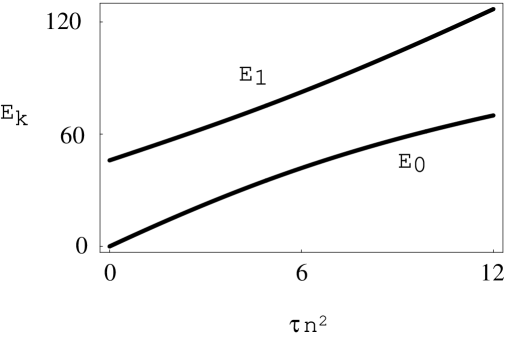
Figure 2: Two lowest eigenvalues of $H(\tau)$ (17): $E_{0,1}$ vs $\tau\,n^{2}$ in the vicinity of avoided crossing for $n=46$ and $q=3$.

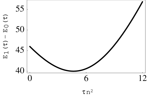
Figure 3: Difference between the two lowest eigenvalues of $H(\tau)$ (17): $E_{1}-E_{0}$ vs $\tau\,n^{2}$ $n=46$ and $q=3$.

IV.1 Numerical analysis

We also performed numerical simulations of the adiabatic spectrum with Hamiltonian (17). In Fig. 2, we plot the ground state and the first excited state energies as functions of the dimensionless ”time” $\eta=\tau n^{2}$ for even values of $n$. According to the above discussion, in this case the ground state is not degenerate and the energy level differnce exhibits a non-monotonic behavior (cf. Fig. 3) leading to the polynomial minimal gap $\Delta E_{\min}\sim n$ at $\eta\sim 1$.

Figure 4: Eigenvalues of the Hamiltonian $H(\tau)$ (17) at the avoided-crossing, $\tau=\tau_{c}$; $n=46$, $q=3$.

In Fig. 4 we plot an eigenvalue spectrum of the Hamiltonian $H(\tau)$ at the avoided crossing point, $\tau=\tau_{c}$ for an even value of $n$. For $k\gg 1$ $E_{k}={\cal O}(n^{3}\,k^{2})$ which corresponds to the scaling analysis in Eqs. (31),(32). Zeeman splitting of a doublet of the two lowest exited energy levels in Fig. 4 is of the order of $n^{3}\tau_{c}={\cal O}(n)$.

In Fig.3 we plot the dependence of minimal gap $\Delta E_{\min}$ vs $n$ for even values of $n$ . The insert to this plot corresponds to the dependence of the avoided crossing point $\tau_{c}$ vs $n$.

Using the simple quasi-classical picture presented above it is not difficult to compute the minimum gap in the case of the driver Hamiltonian (13) in terms of the appropriate tunneling exponent and recover the answer given in annealing .

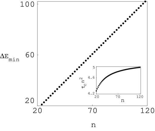
Figure 5: Minimum gap vs $n$ for even $n$. The slope of the graph is 0.86 corresponding approximately to the analytical estimate for $\Delta E_{\min}=(2/3)^{1/2}$ (29). Insert: Scaled position of the avoided crossing point $\tau_{c}n^{2}$ vs $n$. The assymptotic result is $\tau_{c}\,n^{2}\approx 4.98$ at $n\gg 1$.

V Conclusion

We show that macroscopic tunneling in QAA with the symmetrized cost function can be totally suppressed using a driver Hamiltonian with the ground state extended in the space of a total spin projection onto the direction of computational basis. This leads to a polynomial time complexity of QAA. We give a simple form of a driver Hamiltonian (14) that has the aforementioned property and therefore makes the algorithm polynomial.

We developed a simple intuitive picture of this phenomenon based on WKB approximation for large spins. It follows from the analysis that the results will hold for any form of $f(w)$ that is sufficiently smooth on the scale $w\sim 1$. We conjecture that this phenomenon holds even if the cost function $E_{\bf z}$ is symmetrical with respect to the permutation of bits but is not expressed only throught the Hamming weight of a string.

We also argue using a picture of QAA as a quantum local search Vazirani02 ; ST that suppression of tunneling barriers with the operator $S_{x}^{2}$ changes the global neighborhood properties for QAA in a very profound way that can have an effect on the algorithm complexity for a larger class of cost functions, $E_{\bf z}=f(w_{\bf z})+\Delta f_{\bf z}$ where $\Delta f_{\bf z}$ breaks the symmetry between the bits. In particular, it can be large for those states $|{\bf z^{\prime}}\rangle$ that have exponentially small overlap $|\langle{\bf z^{\prime}}|\Psi_{0}(\tau)\rangle|$ with adiabatic ground states at all times (cf. Sec. 7.3 of Vazirani02 ).

A possible generalization of the above analysis is related to random optimization problems with frustration, such as NP-hard problems and corresponding spin glass models. Exponential complexity of quantum adiabatic evolution algorithms for these problems is not necessarily related to tunneling but rather to the quantum diffusion phenomenon associated with the rapid falloff of correlations in the bit-structure with growing size of neighborhood around a given string ST . The role of the tunneling and collective phenomena involving the low cost configurations in the performance of the quantum adiabatic evolution algorithms in random NP-hard is yet to be analyzed.

VI Acknowledgments

We wish to thank Edward Farhi, Samuel Gutmann, Andrew Childs ( MIT), and Umesh Vazirani ( UC Berkley) for stimulating discussions. We also wish to thank Alex Burin (Northwestern University) for turning our attention to Refs. GARG1 ; GARG2 . This research was supported by NASA Intelligent Systems Revolutionary Computing Algorithms program (project No:749-40).

VII Note Added

Shortly after this work was completed, we learned about the work of E.Farhi, J. Goldstone, S. Gutmann farhi_paths wherein another approach was suggested to achieve polynomial complexity of the quantum adiabatic evolution algorithm for the same optimization problem with the symmetrized cost function (8). The algorithm proposed in Ref. farhi_paths is quite different from our algorithm. We believe that the proposal in farhi_paths for random generation of interpolating “paths” $H(t)$ in different trials of the algorithm is a very promising tool. It can perhaps be modified, by including intermediate measurents farhimeas , to become an efficient adaptive algorithm for random NP-hard optimization problems.

However we believe the particular method of achieving polynomial complexity presented in farhi_paths is less robust than ours in the problems with $n$ qubits where the dynamics of the total spin $n/2$ is a key. The difference between the two algorithms is that in our approach a simple universal form of the driver Hamiltonian guarantees that the minimum gap scales polynomially in the problem size for a broad class of symmetrized cost functions $f(w)$. Also, by construction our method does not require a specific knowledge of the solution, or even a specific form of the cost function $f(w)$.

We also believe that simple quasi-classical approach presented above enables one to study analytically a “volume” in the space of possible interpolating paths farhi_paths that find a solution in polynomial time. Detailed study of this issue will be presented elsewhere.

VIII Appendix: Minimum gap estimate using matrix representation

The eigenstates and eigenvectors of the Hamiltonian (17) can be obtained solving from the matrix representation. Choosing $x$ as a quantization axis, we have $S_{z}=\left(-i\right)\left(S_{+}-S_{-}\right)$ and

$$\left(S_{x}^{2}\right)_{m,m} = m^{2},\quad m=-l,-l+1,\ldots,l,$$

$$\left(S_{+}\right)_{m,m-1} = \left(S_{-}\right)_{m-1,m}=\frac{1}{2}\sqrt{\left[l\left(l+1\right)-m\left(m-1\right)\right]}.$$

The full Hamiltonian (17) is given by

$$H\left(\tau\right) = \left(1-\tau\right)nS_{x}^{2}+\tau\left(\frac{n}{2}\right)^{3}h\left(S_{z}\right),$$

$$h\left(S_{z}\right) = \frac{1}{2}\left[\left(q+\frac{4}{3}\right)+\frac{\left(2-q\right)}{l}S_{z}-\frac{q}{l^{2}}S_{z}^{2}+\frac{\left(q-2/3\right)}{l^{3}}S_{z}^{3}\right],$$

and has the following matrix elements

$$\left(H\right)_{m,m} = \left(1-\tau\right)n\ m^{2}+\tau\left(\frac{n}{2}\right)^{3}\frac{1}{2}\left(q+\frac{4}{3}-q\Lambda_{0}\right),$$

$$\left(H\right)_{m,m-1} = \frac{1}{2}\tau\left(\frac{n}{2}\right)^{3}\left[\left(2-q\right)\Lambda_{1}+\left(q-2/3\right)\Lambda_{2}\right],$$ (30)

$$\left(H\right)_{m,m-2} = \frac{1}{2}\tau\left(\frac{n}{2}\right)^{3}\left(-q\right)\Lambda_{3},$$

$$\left(H\right)_{m,m-3} = \frac{1}{2}\tau\left(\frac{n}{2}\right)^{3}\left(q-2/3\right)\Lambda_{4},$$

with

$$\Lambda_{0}\left(l,m\right) = \frac{1}{2l^{2}}\left[l\left(l+1\right)-m^{2}\right],$$

$$\Lambda_{1}\left(l,m\right) = \frac{\left(-i\right)}{2l}\sqrt{l\left(l+1\right)-m\left(m-1\right)},$$

$$\Lambda_{2}\left(l,m\right) = \frac{3i}{4l^{3}}\sqrt{l\left(l+1\right)-m\left(m-1\right)}\left[l\left(l+1\right)-m\left(m-1\right)-1\right],$$

$$\Lambda_{3}\left(l,m\right) = -\frac{1}{4l^{2}}\sqrt{\left[l\left(l+1\right)-m\left(m-1\right)\right]\left[l\left(l+1\right)-\left(m-1\right)\left(m-2\right)\right]},$$

$$\Lambda_{4}\left(l,m\right) = -\frac{i}{2l}\sqrt{\left[l\left(l+1\right)-\left(m-2\right)\left(m-3\right)\right]}\Lambda_{3}\left(l,m\right).$$

One should note that the coefficients $\left\{\Lambda_{k}\right\}$ do not scale with $l=2n$, i.e. $\Lambda_{k}={\cal O}(1)$ for $n\gg 1$. From (30), it follows that the eigenvalue problem $H\left(\tau\right)\Psi_{k}=E_{k}\left(\tau\right)\Psi_{k}$ is rescaled for $n\gg 11$ in terms of dimensionless variables $\eta=\tau n^{2}$ and $\widetilde{E}_{k}\left(\tau\right)=E_{k}\left(\tau\right)/n$ as

$$\widetilde{H}\left(\tau\right)\Psi_{k}=\widetilde{E}_{k}\left(\tau\right)\Psi_{k},$$ (31)

with

$$\left(\widetilde{H}\right)_{m,m} = m^{2}+\frac{\eta}{16}\left(q+\frac{4}{3}-q\Lambda_{0}\right),$$

$$\left(\widetilde{H}\right)_{m,m-1} = \frac{\eta}{16}\left[\left(2-q\right)\Lambda_{1}+\left(q-2/3\right)\Lambda_{2}\right],$$ (32)

$$\left(\widetilde{H}\right)_{m,m-2} = \frac{\eta}{16}\left(-q\right)\Lambda_{3},$$

$$\left(\widetilde{H}\right)_{m,m-3} = \frac{\eta}{16}\left(q-2/3\right)\Lambda_{4},$$

implying that matrix elements of $\widetilde{H}$ do not scale with $n$ and neither do the eigenvalues of $\widetilde{H}$. It is strighforward to obtain an estimate for the minimum gap from the above equation using a Brillouin-Wigner perturbation theory in parameter $\eta$. If one uses a 3-level truncation scheme, ($m=0,\pm 1$), and sets $q=3$ then a quasi-classical estimate (29) can be recovered to the leading order in $n$.

References

- (1) E. Farhi, J. Goldstone, S. Gutmann, and M. Sipser, “Quantum Computation by Adiabatic Evolution”, arXiv:quant-ph/0001106, (2002).
- (2) E. Farhi, J. Goldstone, S. Gutmann, J. Lapan, A. Lundgren, and D. Preda, “A quantum adiabatic evolution algorithm applied to random instances of NP-complete problem”, Science, 292, 472 (2001).
- (3) E. Farhi, J. Goldstone, and S. Gutmann, “A numerical study of the performance of a quantum adiabatic evolution algorithm for Satisfiability”, arXiv:quant-ph/0007071.
- (4) A. M. Childs, E. Farhi, J. Goldstone, and S. Gutmann, “Finding cliques by quantum adiabatic evolution”, arXiv:quant-ph/0012104.
- (5) W. Van Dam, M. Mosca, U. Vazirani, ”How Powerful is adiabatic Quantum Computation?”, arXiv:quant-ph/0206003.
- (6) C. Bennett, E. Bernstein, G. Brassard, and U. Vazirani,”Sterngths and weaknesses of quantum computing”, SIAM Journal of Computing, 26, pp. 1510-1523 (1997); arXiv:quant-ph/9701001
- (7) E. Farhi, J. Goldstone, S. Gutmann, “Quantum adiabatic evolution algorithms versus aimulated annealing”, arXiv:quant-ph/0201031.
- (8) W. Van Dam, M. Mosca, U. Vazirani, ”How Powerful is Idiabatic Quantum Computation?”, FOCS 2001.
- (9) U. Vazirani, ”Quantum Adiabatic algorithms”, talk on ITP Conference on Quantum Information, (UC Berkley, Desember, 2001), http://online.itp.ucsb.edu/ online/qinfoc01
- (10) W. Wernsdorfer, R. Sessoli, “Quantum phase interference and parity effects in magnetic molecular clusters”, Science, 284, p.133 (1999).
- (11) Y. Fu and P.W. Anderson, “Application of statistical mechanics to NP-complete problems in combinatorial optimization”, J. Phys. A: Math. Gen. 19, 1605-1620 (1986).
- (12) M. Mezard, G. Parizi, and M.A. Virasoro, Spin Glass Theory and Beyond, (Wold Scientific, Singapore, 1987).
- (13) R. Monasson and R. Zecchina, “Entropy of the K-Satisfiability problem”, Phys. Rev. Lett, 76, p.3881 (1996); ibid, “Statistical mechanics of the random K-satisfiability problem”, Phys. rev. E 56, p.1357 (1997).
- (14) When this work was completed we read the paper farhi_paths in which a quite different proposal for the polynomial time QAA was suggested for the same type of optimization problems. We provide a brief discussion and comparision of the approaches in Sec. VII.
- (15) E. Farhi, J. Goldstone, S. Gutmann, “Quantum adiabatic evolution algorithms with different paths”, arXiv:quant-ph/0208135.
- (16) V. N. Smelyansky and U. V. Toussaint, ”Number Partitioning via Quantum Adiabatic Computation”, arXiv:quant-ph/0202155.
- (17) E. M. Chudnovsky and D. A. Garanin, “Quantum tunneling of Magnetization in small ferromagnetic particles”, Phys. Rev. Lett., v.79, 4469 (1997).
- (18) A. Garg, Europhys. Lett., v.22, 205 (1993).
- (19) M. Stone, K. Park, and A. Garg, Journ. Math. Phys., v.41, 8025 (2000).
- (20) L. D. Landau and E. M. Lifshitz, Quantum Mechanics, (Pergammon, 1992).
- (21) A. M. Childs, E. Deotto, E. Farhi, J. Goldstone, S. Gutmann, A. J. Landhal, “Quantum search by measurment”, arXiv:quant-ph/0204013.