Abstract

It is shown how the phase-damping master equation, either in Markovian and nonMarkovian regimes, can be obtained as an averaged random unitary evolution. This, apart from offering a common mathematical setup for both regimes, enables us to solve this equation in a straightforward manner just by solving the Schrödinger equation and taking the stochastic expectation value of its solutions after an adequate modification. Using the linear entropy as a figure of merit (basically the loss of quantum coherence) the distinction of four kinds of environments is suggested.

1 Introduction

The principle of quantum superposition is at the base both of important issues concerning the conceptual foundations of quantum mechanics [1] and of potential direct technological applications of quantum theory [2, 3]. In particular the preservation and dissapearance of these quantum superpositions play a central role in topics like the quantum-to-classical transition [4] and the performance of some quantum information processing tasks [5]. Physically this decoherence has its origins in the pervasive effect of the surrounding environment. Mathematically it is expressed by means of master equations (ME hereafter), that is evolution equations for the reduced density operator of the system which are usually obtained after some careful assumptions [6].

By and large two main approaches can be followed to study these master equations [7], namely a constructive and an axiomatic approach. In the former one begins considering the joint system-environment degrees of freedom and finally pursues reasonable and manageable approximations to obtain the master equation of the system. This approach usually falls into mathematical difficulties hard to deal with, though some limit situations have been satisfactorily dealt with [8, 9]. On the other hand, the latter approach poses a set of reasonable and physically motivated assumptions [10, 11] and then derive the general form for the master equation of systems satisfying that set of axioms. Though most of ME of practical relevance fall into this category (see e.g. [12]), the range of applicability of this approach is limited by definition, especially regarding one of its fundamental axioms, namely the semigroup condition (Markovianity).

In an attempt to embrace also nonMarkovian situations we have combined well-known stochastic methods jointly with common tools of functional analysis employed in quantum mechanics [13, 14] to state the following result: Any Lindblad-type evolution with selfadjoint Lindblad operators, whether Markovian or nonMarkovian, can be understood as an averaged random unitary evolution. This result, whose fully-fledged mathematical proof is provided elsewhere [15], reveals the fact that the Lindblad structure of ME for the case of selfadjoint Lindblad operators is beyond the Markov approximation and can also be recovered in nonMarkovian situations.

Here we exploit the mathematical advantages of this approach to study the loss of coherence described by the phase-damping ME and identify different types of environments using the linear entropy as a figure of merit.

2 The Phase-Damping Master Equation as an Averaged Random Evolution

The generalized phase-damping ME reads

$$\frac{d\rho(t)}{dt}=-i[H,\rho(t)]-\frac{\dot{\lambda}(t)}{2}[H,[H,\rho(t)]]$$ (1)

where $H$ denotes the Hamiltonian of the system and we have allowed $\dot{\lambda}(t)$ to be any nonnegative real function. In general eq. (1) denotes a nonMarkovian evolution reducing to a Markovian one only when $\dot{\lambda}(t)=\lambda\equiv\textrm{const}$. Eq. (1) is a Lindblad-type ME with selfadjoint Lindblad operators and consequently following the result stated above can be obtained as an averaged random unitary evolution. The proof for this case is straighforward. Let $U(t)=e^{-itH}$ $(\hbar=1)$ be the unitary evolution operator of the quantum system under study. Let us now define the random unitary evolution operator $U_{st}(t)=e^{-itH-iH\int_{0}^{t}\sigma(s)d\mathcal{B}_{s}}$, where $\sigma(t)$ denotes an arbitrary real function and $\mathcal{B}_{t}$ denotes standard real Brownian motion [16], thus $\int_{0}^{t}\sigma(s)d\mathcal{B}_{s}$ will denote the well-known Ito integration. Now let the density operator $\rho(t)$ be defined as

$$\rho(t)=\mathbb{E}[U_{st}(t)\rho(0)U_{st}^{\dagger}(t)]$$ (2)

where $\mathbb{E}$ denotes expectation value with respect to the probability measure of $\mathcal{B}_{t}$. Then after making some calculations one can see that $\rho(t)$ satisfies the ME (1) with $\dot{\lambda}(t)=\sigma^{2}(t)$.

3 Interference Damping for Plane Waves

One of the immediate consequences of the above procedure arises by realizing that the solutions to the ME (1) can be obtained by performing the substitution $t\to t+\int_{0}^{t}\sigma(s)d\mathcal{B}_{s}$ in the unitary solutions and then taking the stochastic expectation value.

We will illustrate these ideas with the study of the interference pattern between two equally-weighted plane waves with momentum $k_{1}$ and $k_{2}$ respectively evolving under the ME (1). The unitary solution can be obtained elementarily either by solving the Schrödinger equation for the state vector or by solving the Liouville-von Neumann equation for the density operator or by resorting to the Wigner characteristic function [17] $\chi(\lambda,\mu)=\textrm{Tr}[\rho(t)e^{i(\mu p+\lambda q)}]$ where $q$ and $p$ are the position and momentum operators (cf. also [18]). The interference pattern is provided by the well-known expression

$$I(x,t)=1+\cos[(k_{1}-k_{2})x-\frac{k_{1}^{2}-k_{2}^{2}}{2m}t]$$ (3)

This pattern is changed when the initial superposition evolves under eq. (1) and accordingly the solution is more involved. One can again resort to the Wigner characteristic function $\chi(\lambda,\mu)$ to obtain the solution [18], but using our previous result one can immediately arrive at the desired expression:

$$I(x,t)\to\bar{I}(x,t)=\mathbb{E}[I(x,t+\int_{0}^{t}\sigma(s)d\mathcal{B}_{s})]$$ (4)

Then knowing that (cf. appendix)

$$\mathbb{E}\left[\cos\left[\frac{k_{1}^{2}-k_{2}^{2}}{2m}\left(t+\int_{0}^{t}\sigma(s)d\mathcal{B}_{s}\right)\right]\right] = e^{-\frac{1}{2}\left(\frac{k_{1}^{2}-k_{2}^{2}}{2m}\right)^{2}\int_{0}^{t}\sigma^{2}(s)ds}\cos\left[\frac{k_{1}^{2}-k_{2}^{2}}{2m}t\right]$$

$$\mathbb{E}\left[\sin\left[\frac{k_{1}^{2}-k_{2}^{2}}{2m}\left(t+\int_{0}^{t}\sigma(s)d\mathcal{B}_{s}\right)\right]\right] = e^{-\frac{1}{2}\left(\frac{k_{1}^{2}-k_{2}^{2}}{2m}\right)^{2}\int_{0}^{t}\sigma^{2}(s)ds}\sin\left[\frac{k_{1}^{2}-k_{2}^{2}}{2m}t\right]$$

we get

$$\bar{I}(x,t)=1+e^{-\frac{1}{2}\left(\frac{k_{1}^{2}-k_{2}^{2}}{2m}\right)^{2}\int_{0}^{t}\sigma^{2}(s)ds}\cos[(k_{1}-k_{2})x-\frac{k_{1}^{2}-k_{2}^{2}}{2m}t]$$ (6)

Different interference patterns are obtained corresponding to different types of environments. Note that since the Markovian approximation is not assumed, we have now gained some generality.

4 Different Types of Environment

We will investigate the time evolution of the linear entropy in order to study the progressive loss of coherence of systems driven by the ME (1). To avoid mathematical nuisances because of the lack of normalizability of plane waves, let us focus upon an initial gaussian wave packet

$$\psi(x,0)=\frac{1}{(2\pi\sigma^{2}_{0})^{1/4}}e^{-\frac{x^{2}}{4\sigma^{2}_{0}}}$$

Under equation (1) the linear entropy $S_{lin}(t)$ of the system can be calculated:

$$S_{lin}(t)=1-\frac{1}{\sqrt{16\pi}}\frac{4m\sigma_{0}^{2}}{\lambda^{1/2}(t)}\int_{0}^{\infty}\frac{dy}{y}e^{-\frac{4m\sigma_{0}^{2}}{\lambda^{1/2}(t)}y}\textrm{erf}(y)dy$$ (7)

where $\lambda(t)=\int_{0}^{t}\sigma^{2}(s)ds$. Note that the previous integral exists for all possible choices of $\sigma(t)$ since the integrand ($\equiv g(y,t)$) is continuous in $\mathbb{R}^{+}$ and

$$\lim_{y\to 0}g(y,t) = \frac{2}{\sqrt{\pi}}$$

$$\lim_{y\to\infty}g(y,t) = 0$$

$$g(y,t) \sim \frac{e^{-\frac{4m\sigma_{0}^{2}}{\lambda^{1/2}(t)}y}}{y}\quad y\gg 1$$

Also notice that the second term in (7) $(\equiv I(t))$ is bounded from above and from below:

$$0\leq I(t)\leq 1\Rightarrow 0\leq S_{lin}(t)\leq 1$$ (8)

In particular $S_{lin}(t)=0$ if and only if $\lambda(t)=0$, i.e. one always obtains a decohering process. Immediately one can distinguish four different kinds of situations:

• $\lambda(t)=\lambda t$. This is the usual Markovian approximation. In this case (cf. also [4])

  $$S_{lin}(t)\stackrel{{\scriptstyle t\to\infty}}{{\longrightarrow}}1$$ (9)

• $\lambda(t)\stackrel{{\scriptstyle t\to\infty}}{{\longrightarrow}}\lambda_{0}$. Let us call it SubMarkovian regime. Now the linear entropy reaches a maximum value $S_{0}<1$, thus the initial coherence is partially preserved.

• $\lambda(t)\stackrel{{\scriptstyle t\to\infty}}{{\longrightarrow}}\infty$ but $\frac{\lambda(t)}{t}\stackrel{{\scriptstyle t\to\infty}}{{\longrightarrow}}0$. Let us call it type-I SuperMarkovian regime. Now as in the Markovian case $S_{lin}(t)\to 1$ but at a slower pace. This allows the system to preserve a higher degree of coherence at a given time.

• $\lambda(t)\stackrel{{\scriptstyle t\to\infty}}{{\longrightarrow}}\infty$ and $\frac{\lambda(t)}{t}\stackrel{{\scriptstyle t\to\infty}}{{\longrightarrow}}\infty$. Let us call it type-II SuperMarkovian regime. This is the most destructive case since $S_{lin}(t)\to 1$, that is coherence is completely lost and even faster than in the usual Markovian case.

The four situations are qualitatively represented in Fig. 1.

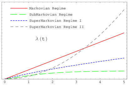
Figure 1: Decoherence functions for different types of environment. See text.

5 Conclusions

We have derived the phase-damping master equation using stochastic calculus and subsequently solve it using the advantages of this procedure. These advantages run from embracing under the same mathematical formalism both Markovian and nonMarkovian evolutions (thus allowing us to deal with more general physical situations) to providing a new method to solve this equation. The great advantage of this procedure comes out from the fact that you only need to solve the unitary evolution equation, which can be done for the state vector instead of dealing with the density operator. This represents a computational advantage. Once the unitary solution is known all one has to do is to find the stochastic expectation value of this solution after modifying it with the appropiate random factor (see above).

Using then the linear entropy as a figure of merit we have found four types of environments according to the rate of loss of coherence they induce upon the system. In particular it may be concluded that what we have called SubMarkovian and Type-I SuperMarkovian regimes appear as better choices to perform quantum-informational and quantum-computational tasks than the usual Markovian environment. Now the physical conditions should be provided to properly identify what these kinds of environment are.

It should be noticed that as a by-product of this approach, independently of the function $\sigma(t)$ used to describe the system-environment response, a positive and nondecreasing rate of decoherence is always obtained, which indicates that it is an irreversible process. Thus under the conditions in which the phase-damping master equation is valid to describe the evolution of a system, coherence can never be recovered from the environment, whether this is Markovian or nonMarkovian.

Appendix A Some Computational Notes

In order to compute the expectation values (LABEL:ExpValCos) and (LABEL:ExpValSin) it is necesarry to know the nth order moments of the real-valued stochastic process $X_{t}=t+\int_{0}^{t}\sigma(s)d\mathcal{B}_{s}$. It is simple to find $\beta_{n}(t)\equiv\mathbb{E}[X_{t}^{n}]$ using Ito’s formula [16] upon $\phi(X_{t})=X_{t}^{n}$:

$$d\phi(X_{t}) = (nX_{t}^{n-1}+\frac{n(n-1)}{2}X_{t}^{n-2}\sigma^{2}(t))dt+nX_{t}^{n-1}\sigma(t)d\mathcal{B}_{t}\Rightarrow$$

$$\Rightarrow\frac{{d\beta}_{n}(t)}{dt} = n\beta_{n-1}(t)+\frac{n(n-1)}{2}\beta_{n-2}(t)\sigma^{2}(t)\quad n\geq 2$$ (10)

Since $\beta_{0}(t)=1$ and $\beta_{1}(t)=0$ it is straighforward to recursively arrive at

$$\beta_{2n}(t) = \frac{(2n)!}{2^{n}n!}\lambda^{n}(t)$$ (11a)

$$\beta_{2n+1}(t) = 0$$ (11b)

where $\lambda(t)\equiv\int_{0}^{t}\sigma^{2}(s)ds$.

To arrive at (7) the following integral is needed which can be obtained by means of already tabulated integrals [19]:

$$\int_{0}^{\pi}e^{-z\cos^{2}\theta}d\theta=\sqrt{\frac{\pi}{z}}\textrm{erf}(\sqrt{z})$$ (12)

References

- [1] B. d’Espagnat. Conceptual Foundations of Quantum Mechanics. 2nd compl. rev. and enl. ed. Addison-Wesley, New York, 1976.
- [2] H.-K. Lo, S. Popescu, and T. Spiller, editors. Introduction to Quantum Computation and Information. World Scientific, Singapore, 1998.
- [3] D. Bouwmeester, A. Ekert, and A. Zeilinger (eds.). The Physics of Quantum Information. Springer, Berlin, 2000.
- [4] D. Giulini, E. Joos, C. Kiefer, J. Kupsch, I.-O. Stamatescu, and H.D. Zeh. Decoherence and the appearance of a classical world in quantum theory. Springer-Verlag, Berlin, 1996.
- [5] I.L. Chuang and M.A. Nielsen. Quantum Computation and Quantum Information. Cambridge University Press, Cambridge, 2000.
- [6] C. Cohen-Tannoudji, J. Dupont-Roc and G. Grynberg. Atom-Photon Interactions. Basic Processes and Applications. Wiley Interscience, New York, 1992.
- [7] R. Alicki. Lecture given at the 38th Winter School of Theoretical Physics, Ladek, Poland, 2002.
- [8] E.B. Davies. Quantum Theory of Open Systems. Academic Press, London, 1976.
- [9] V. Gorini, A. Frigerio, M. Verri, A. Kossakowski, and E.C.G. Sudarshan. Rep. Math. Phys. 13, 149 (1978).
- [10] G. Lindblad. Commun. Math. Phys. 48, 119 (1976).
- [11] V. Gorini, A. Kossakowski, and E.C.G. Sudarshan. J. Math. Phys. 17, 821 (1976).
- [12] A. Isar, A. Sandulescu and W. Scheid. J. Math. Phys. 34, 3887 (1993).
- [13] E. Prugovecki. Quantum Mechanics in Hilbet Space. Academic Press, New York, 2nd edition, 1981.
- [14] N.T. Dunford and J.T. Schwartz. Linear Operators. Part II: Spectral Theory. Interscience, New York, 1963.
- [15] D. Salgado and J.L. Sánchez-Gómez, quant-ph/0208175.
- [16] B. Oksendal. Stochastic Differential Equations. 5th ed. Springer, Berlin, 1998.
- [17] W.H. Louisell. Quantum Statistical Properties of Radiation. Wiley, New York, 1973.
- [18] C.M. Savage and D.F. Walls. Phys. Rev. A, 32, 3487 (1985).
- [19] I.S. Gradshteyn and I.M. Rizhik. Table of Integrals, Series and Products. 5h ed. Academic Press, London, 1994.