Continuous quantum nondemolition feedback and unconditional atomic spin squeezing

Abstract

We discuss the theory and experimental considerations of a quantum feedback scheme for producing deterministically reproducible spin squeezing. Continuous nondemolition atom number measurement from monitoring a probe field conditionally squeezes the sample. Simultaneous feedback of the measurement results controls the quantum state such that the squeezing becomes unconditional. We find that for very strong cavity coupling and a limited number of atoms, the theoretical squeezing approaches the Heisenberg limit. Strong squeezing will still be produced at weaker coupling and even in free space (thus presenting a simple experimental test for quantum feedback). The measurement and feedback can be stopped at any time, thereby freezing the sample with a desired amount of squeezing.

1 Introduction

Squeezed spin systems [1] of atoms and ions have attracted considerable attention in recent years due to the potential for practical applications, such as in the fields of quantum information [2] and high precision spectroscopy [3]. The basic principle is that the quantum correlations of squeezed spin states will outperform classical states in the same fashion as squeezed optical fields. Moreover, spin squeezing is related to the fundamental concept of entanglement [4] and specifically represents many-particle entanglement [5, 6]. There have been a number of proposals for spin squeezing and a variety of experimental results are now being observed.

One area of research involves the use of broadband squeezed light [7], in which case the squeezed spin state is generated via quantum state transfer between nonclassical light and an atomic ensemble. This method has recently produced weakly squeezed states [8]. In analogy with nonlinear optics, another proposal is the collisional interactions in a Bose-Einstein condensate (BEC). These represent a nonlinearity which will dynamically generate spin squeezing in the trapped state [5, 9] and also any out-coupled beams [10]. There are also schemes for direct coupling to the entangled state through intermediate states such as collective motional modes for ions [11] or molecular states for atoms [12]. A related proposal is the photodissociation of molecular condensates [13] in analogy with the down-conversion process in quantum optics. There has also been experimental evidence that the ground state of a BEC confined in an optical lattice can be produced in an atom-number squeezed state [14].

Production of spin squeezed states via quantum nondemolition (QND) detection has also been considered [15] and spin noise reduction using this method has been experimentally observed [16]. QND measurements are also involved in the proposal [17] for the entanglement of two macroscopic atomic samples, which has recently been achieved [18]. These schemes represent conditional squeezing of the atomic ensembles. However, it would be preferable to develop unconditional, i.e., deterministically reproducible, squeezing especially in regard to the field of quantum information. The ideal would be to prepare the same squeezed spin state regardless of the measurement record.

In this work, we develop the idea introduced in Ref. [19] of achieving deterministic spin squeezing via quantum feedback, in analogy with optical squeezing via quantum feedback [20]. Monitoring the output of a probe field sensitive to atoms in a particular internal state will conditionally squeeze the collective angular momentum of the sample. Unconditional squeezing is then obtained by using the measurement results to continuously drive the system into the desired, deterministic, squeezed spin state. We show (not done previously) that measurement schemes based in an optical cavity or free space both lead to the same system dynamics, i.e., that due to a QND measurement of one collective spin operator.

It has been shown that a series of QND measurements followed by feedback can ensure perfect agreement between the number of atoms in two internal sates [21]. However this analysis does not take into account the quantum effects of the measurement back-action and feedback dynamics. The QND detection in our scheme will conditionally produce quantum correlations between the atoms, but it is not clear whether the feedback dynamics (introduced to produce unconditional squeezing) will adversely affect these correlations. In this paper, we perform a full quantum analysis to look at this question, and find the quantum limit to squeezing for the ideal situation of no atom losses. Further, we qualitatively explore how this limit is affected by losses and what this implies experimentally.

In Sec. 2 we briefly review the definition of squeezed spin states and the types of nonlinear interactions which produce them. The main body of this paper, Sec. 3, details the quantum dynamics of the continuous measurement and feedback scheme (3.1 and 3.2) and determines an experimentally feasible approach to implementing the required feedback. It also includes the effective nonlinear interactions produced by this scheme (3.3), details the numerical work (3.4), and a discussion of experimental considerations (3.5). Sec. 4 concludes and an appendix covers the results of inefficient measurement.

2 Squeezed spin systems

The collective properties of $N$ two-level atoms are conveniently described by a spin-$J$ system [22]. This is a collection of $2J=N$ spin-$\frac{1}{2}$ particles where the internal states $|{1}\rangle$ and $|{2}\rangle$ of the $k$th atom represent the two states of the $k$th spin-$\frac{1}{2}$ particle. The collective angular momentum operators, ${\mathbf{J}}$, are given by $J_{\alpha}=\sum_{k=1}^{N}j^{(k)}_{\alpha}(\alpha=x,y,z)$, where $j^{(k)}_{\alpha}=\sigma_{\alpha}^{(k)}/2$ and $\sigma_{\alpha}^{(k)}$ are the Pauli operators for each particle. ${\mathbf{J}}$ obey the cyclic commutation relations $[J_{x},J_{y}]=i\epsilon_{xyz}J_{z}$ and the corresponding uncertainty relation $(\Delta J_{y})^{2}(\Delta J_{z})^{2}\geq\mbox{$\frac{1}{4}$}|\left\langle{J_{x}}\right\rangle|^{2}$.

Equivalently, defining the operators $a^{\dagger}_{i}~{}(i=1,2)$ for creating atoms in a particular internal state, we have $J_{z}=\mbox{$\frac{1}{2}$}(a^{\dagger}_{2}a_{2}-a^{\dagger}_{1}a_{1}),J_{+}=a^{\dagger}_{2}a_{1},J_{-}=a^{\dagger}_{1}a_{2}$ and the total number operator $a^{\dagger}_{1}a_{1}+a^{\dagger}_{2}a_{2}$ equals a constant, i.e., $N$. $J_{z}$ represents half the total population difference and is a quantity which can be measured, for example by dispersive imaging techniques [23]. $J_{x}\equiv(J_{+}+J_{-})/2$ and $J_{y}\equiv(J_{+}-J_{-})/2i$ represent the two quadrature-phase amplitudes of the collective dipole moment.

For a coherent spin state (CSS) of a spin-$J$ system, all the elementary spins are pointing in the same mean direction. Such a state satisfies the minimum uncertainty relationship with the variance of the two components normal to the mean direction equal to $J/2$. If quantum-mechanical correlations are introduced among the atoms it is possible to reduce the fluctuations in one direction at the expense of the other. This is the idea of a squeezed spin state (SSS) introduced by Kitagawa and Ueda [1], i.e. the spin system is squeezed when the variance of one spin component normal to the mean spin vector is smaller than the standard quantum limit (SQL) of $J/2$.

There are many ways to characterize the degree of spin squeezing in a spin-$J$ system. We will use the criteria of Sørensen and co-workers [5] and Wang [24], where the squeezing parameter is given by

$$\xi^{2}_{{\mathbf{n}}_{1}}=\frac{N(\Delta J_{{\mathbf{n}}_{1}})^{2}}{\left\langle{J_{{\mathbf{n}}_{2}}}\right\rangle^{2}+\left\langle{J_{{\mathbf{n}}_{3}}}\right\rangle^{2}},$$ (1)

where $J_{\mathbf{n}}\equiv{\mathbf{n}}\cdot{\mathbf{J}}$ and ${\mathbf{n}}_{i}(i=1,2,3)$ are orthogonal unit vectors. Systems with $\xi^{2}_{\mathbf{n}}<1$ are spin squeezed in the direction ${\mathbf{n}}$ and it has also been shown that this indicates the atoms are in an entangled state [5, 6]. This parameter also has the appealing property that $\xi^{2}_{x}=\xi^{2}_{y}=\xi^{2}_{z}=1$ for a CSS [24].

It is well known that quadrature squeezing in optical or bosonic systems can be generated in a nonlinear Kerr ($\chi^{(3)}$) medium. Kitagawa and Ueda [1] identified similar nonlinear Hamiltonians that lead to squeezing in spin systems, namely

$$H_{1} = \chi J_{z}^{2},$$ (2)

$$H_{2} = \chi(J_{+}^{2}-J_{-}^{2})/2i=\chi(J_{x}J_{y}+J_{y}J_{x}),$$ (3)

which can be seen as third-order nonlinear processes if we write $\mathbf{J}$ in terms of the atomic creation and annihilation operators. $H_{1}$ can be thought of as twisting the $z$ axis of the quasiprobability distribution. $H_{2}$ is then “two-axis countertwisting”, where the two axes bisecting the $x$ and $y$ axes are simultaneously twisted in opposite directions. Several recent studies have shown that $H_{1}$ describes the nonlinear spin interactions in a two-component Bose condensate [5, 9].

As indicated in Ref. [1], the variance of the squeezed spin component, and hence Eq. (1), decreases to a minimum value corresponding to the maximally squeezed spin state before increasing again. The nonlinear interactions of Eqs. (2) and (3) twist the quasiprobability distribution of the spin state into, and then past, the optimally squeezed distribution. This is because the interactions can not simply be “turned off” when the optimal squeezing is reached. In the limit of large sample size, the minimum squeezing parameter for these interactions scale, respectively, as $H_{1}:\xi^{2}\propto N^{-2/3}$ and $H_{2}:\xi^{2}\propto N^{-1}$.

In our proposal the required nonlinear interactions between atoms are introduced by a continuous measurement and feedback scheme. We not only find that the minimum squeezing parameter scales as $N^{-1}$ (in the appropriate coupling regime), but that due to the nature of the scheme, the atomic sample could essentially be frozen in this maximally squeezed state (or less squeezed states) simply by ceasing the measurement and feedback.

3 Quantum feedback scheme

Let the two internal states of each atom, $|{1}\rangle$ and $|{2}\rangle$, be the degenerate magnetic sublevels of a $J=\mbox{$\frac{1}{2}$}$ state, for example, the ground state of an alkali atom. For such atoms, transitions to the $J=\mbox{$\frac{1}{2}$}$ excited states could then be employed for the QND measurement, as shown in Fig. 1$(b)$. This figure shows an idealized experimental schematic for our QND measurement and feedback scheme $(a)$, and the corresponding probe and driving transitions for each atom $(b)$. The details of this scheme are presented in the following two sub-sections.

We assume the atomic sample is prepared such that all the atoms are in one of their internal states and the temperature is very low ($T\approx 0$) such that we can separate out (and ignore) the spatial degrees of freedom. A fast $\pi/2$-pulse is then applied, coherently transferring all atoms into an equal superposition of the two internal states, which is an eigenstate of the $J_{x}$ operator with eigenvalue $J$. As described earlier, the CSS is a minimum uncertainty state so in this case variances of both $J_{z}$ and $J_{y}$ are $J/2$.

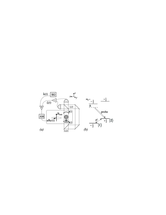
Figure 1: $(a)$ Schematic experimental configuration. A cavity field (equally damped at rate $\kappa/2$) of amplitude $i|\beta|$ interacts with the atomic sample. The photocurrent $I_{c}(t)$ from the homodyne detection of the cavity output is combined with $\lambda(t)$ produced by a signal generator (SG). The combined signal controls the amplitude (AM) of an rf magnetic field that, together with a static field, drives $J_{y}$. $(b)$ Single atom diagram. A static B-field lifts the degeneracy of the magnetic sublevels. The far-detuned probe field monitors the collective population in state $|{2}\rangle$ (and hence $J_{z}$). The radio frequency (rf) driving field, applied perpendicularly to the static field direction, induces magnetic dipole transitions between $|{1}\rangle$ and $|{2}\rangle$ (thus driving $J_{y}$).

3.1 Measurement

The feedback scheme is based on a quantum nondemolition measurement of the atom number difference between the states $|{1}\rangle$ and $|{2}\rangle$. The quantity to be measured is thus represented by the operator $J_{z}$. Firstly, we consider placing the atomic sample in a strongly driven, heavily damped, optical cavity, as shown in Fig. 1$(a)$. The cavity field is assumed to be far off resonance with respect to transitions probing state $|{2}\rangle$, see Fig. 1$(b)$. This dispersive interaction causes a phase shift of the cavity field proportional to the number of atoms in $|{2}\rangle$. Thus, a QND measurement of $J_{z}$ (since $N$ is conserved) is effected by the homodyne detection of the light exiting the cavity [25].

In general, the interaction of a single atom with this far-detuned probe field is given by the Hamiltonian

$$V=\hbar\Omega^{2}(j_{z}+\mbox{$\frac{1}{2}$})/4\Delta$$ (4)

where $\Omega$ is the Rabi frequency and $\Delta$ is the detuning. In the cavity configuration with $N$ atoms this becomes $\hbar\chi(J_{z}+N/2)b^{\dagger}b$, where $\chi=g^{2}/4\Delta$, and $g$ is the one-photon Rabi frequency [25], and $b$,$b^{\dagger}$ are the cavity field operators normalized such that $\left\langle{b^{\dagger}b}\right\rangle$ is the mean photon number in the cavity. Note that we can choose an initial cavity detuning $-N\chi/2$ to eliminate the $N$ dependent term. For strong coherent driving we can use the semiclassical approximation $b\to i|\beta|+b$, where $b$ now represents small quantum fluctuations around the classical amplitude $i|\beta|$. The interaction is thus

$$H_{\rm cav}=\hbar\chi|\beta|J_{z}(-ib+ib^{\dagger}),$$ (5)

where we have ignored the $\hbar\chi|\beta|^{2}J_{z}$ term by choosing an initial atomic detuning of $-\chi|\beta|^{2}$.

We assume that the cavity field is damped through both mirrors at rate $\kappa/2$, as shown in Fig. 1$(a)$. The master equation for the combined atom-field system due to the interaction in Eq. (5) is thus given by

$$\dot{\rho}_{\rm tot}=-\chi|\beta|[J_{z}(b-b^{\dagger}),\rho_{\rm tot}]+\kappa{\cal D}[b]\rho_{\rm tot},$$ (6)

where ${\cal D}[r]\rho\equiv r\rho r^{\dagger}-(r^{\dagger}r\rho+\rho r^{\dagger}r)/2$. Following the procedure of Sec. VII in Ref. [20] we can adiabatically eliminate the cavity dynamics if the cavity decay rate $\kappa\gg\chi|\beta|\Delta J_{z}$, which requires $\kappa\gg\chi|\beta|\sqrt{N}$ (since initial $\Delta J_{z}=\sqrt{J/2}$). The evolution of the atomic system alone is then given by

$$\dot{\rho}=M{\cal D}[J_{z}]\rho,$$ (7)

where $M=4\chi^{2}|\beta|^{2}/\kappa=8\chi^{2}P/\hbar\omega\kappa^{2}$ and $P=\hbar\omega|\beta|^{2}\kappa/2$ is the input local oscillator power and $\omega$ the frequency. The measurement strength $M$ is equivalent to $2D$ in Eq. (22) of Ref. [25]. Equation (7) represents decoherence of the atomic system due to photon number fluctuations in the cavity field, with the result of increased noise in the spin components normal to $J_{z}$.

In the alternative case of a free space QND measurement, the analysis follows more closely that of Sec. IV A in Ref. [26]. From Eq. (4), the interaction for many atoms in the free space limit is $\hbar\theta(J_{z}+N/2)p^{\dagger}p$. Here $\theta$ is the phase shift of the probe field due to a single atom in state $|{2}\rangle$, and is given by $\theta=\hbar\omega\gamma^{2}/8A\Delta I_{\rm sat}$, where $\omega(=2\pi c/\lambda)$ is the probe frequency, $A$ the cross-sectional area, $\gamma$ the spontaneous emission rate and $I_{\rm sat}=2\pi^{2}\hbar\omega\gamma/\lambda^{2}$ for a two-level atom [27]. Note that the field annihilation operators $p,p^{\dagger}$ are normalised such that $\hbar\omega p^{\dagger}p$ is the probe power, i.e., $p^{\dagger}p$ is the photon flux operator with units of $s^{-1}$. The total interaction Hamiltonian (subtracting a phase shift of $\theta/2$ for each atom) is in this case given by

$$H_{\rm free}=\hbar\theta J_{z}p^{\dagger}p.$$ (8)

The back-action on the atomic sample due to this interaction can be evaluated using the techniques of Sec. III B in Ref. [28]. Assuming the probe field is a coherent state of amplitude $i|\varrho|$, the system evolution is

$$\dot{\rho}=|\varrho|^{2}{\cal D}\left[{e^{-i\theta J_{z}}}\right]\rho\simeq M{\cal D}[J_{z}]\rho-i|\varrho|^{2}\theta[J_{z},\rho],$$ (9)

where the approximation requires $\theta\Delta J_{z}\ll 1$, which is equivalent to the requirement that $\theta\sqrt{N}\ll 1$. The measurement strength is now $M=|\varrho|^{2}\theta^{2}=P\theta^{2}/\hbar\omega$, where $P=\hbar\omega\left\langle{p^{\dagger}p}\right\rangle$ is the mean power. The second term above simply causes a frequency shift in the atomic energy level difference, and can be ignored by choosing an initial atomic detuning of $-|\varrho|^{2}\theta$.

In both cases, the evolution of the system due to this type of interaction is given by the same expression $M{\cal D}[J_{z}]\rho$, i.e Eq. (7). The only difference is in the measurement strength, which is given by $M=8\chi^{2}P/\hbar\omega\kappa^{2}$ for a cavity field and $M=\theta^{2}P/\hbar\omega$ for free space. We can specifically look at the conditioned evolution of the system due to the homodyne detection of the probe field (this achieves the measurement of $J_{z}$).

Continuing the analysis for the cavity regime as in [20], the conditioned density operator for the combined systems evolves as

$$d\rho_{\rm tot} = \{-\chi|\beta|[J_{z}(b-b^{\dagger}),\rho_{\rm tot}]+\kappa{\cal D}[b]\rho_{\rm tot}\}dt$$ (10)

$${+}\,dW(t)\sqrt{\eta\kappa}{\cal H}[b]\rho_{\rm tot},$$

where $dW(t)$ is an infinitesimal Wiener increment defined by the Itô rules ${\rm E}[dW(t)]=0$; $[dW(t)]^{2}=dt$, and ${\cal H}[r]\rho\equiv r\rho+\rho r^{\dagger}-\Tr[(r+r^{\dagger})\rho]\rho$. We have also introduced a measurement efficiency $\eta$. For the setup in Fig. 1$(a)$, only one cavity mirror is monitored thus giving $\eta=1/2$ (assuming perfect photodetectors). In principle, however, one could monitor the output of both mirrors (using, e.g., a Faraday isolator at the input mirror) to obtain a perfect measurement, in which case $\eta=1$. We will continue the analysis here with this assumption, and leave the treatment of $\eta\neq 1$ to the Appendix.

Adiabatic elimination as before gives the stochastic master equation (SME) for the conditioned evolution of atomic system:

$$d\rho_{c}=M{\cal D}[J_{z}]\rho_{c}dt+\sqrt{M}dW(t){\cal H}[J_{z}]\rho_{c}.$$ (11)

In this equation $\rho_{c}$ is the density matrix for the atomic system conditioned on a particular realization of the homodyne signal given by

$$I_{c}(t)=2\sqrt{M}\left\langle{J_{z}}\right\rangle_{c}+\zeta(t)$$ (12)

where $\zeta(t)=dW(t)/dt$ is a white noise term satisfying ${\rm E}[\zeta(t)\zeta(t^{\prime})]=\delta(t-t^{\prime})$ and E indicates the ensemble average. The average or unconditioned evolution is simply recovered by averaging over all possible realizations of the current, i.e. $\rho(t)={\rm E}[\rho_{c}(t)]$. Note that these equations (11) and (12) also apply for the perfect homodyne detection of the free space field, with the appropriate $M$.

The dominant effects of the conditioned evolution (11) on the initial CSS are a decrease in the uncertainty of $J_{z}$ (since we are measuring $J_{z}$) with corresponding noise increases in $J_{y}$ and $J_{x}$, and a stochastic shift of the mean $J_{z}$ away from its initial value of zero. The latter shift can be calculated exactly (since $d\left\langle{J_{z}}\right\rangle_{c}\equiv\Tr[J_{z}d\rho_{c}]$):

$$d\left\langle{J_{z}}\right\rangle_{c} = 2\sqrt{M}dW(t)(\Delta J_{z})^{2}_{c}$$ (13)

$$\approx 2\sqrt{M}I_{c}(t)dt\left\langle{J_{z}^{2}}\right\rangle_{c},$$

where the approximation assumes that $\left\langle{J_{z}}\right\rangle_{c}\approx 0$ (such that $I_{c}(t)\approx dW/dt$) which will apply in the next section. In effect, Eq. (13) is equivalent to a stochastic rotation of the mean spin about the $y$ axis by an angle $d\phi\approx d\left\langle{J_{z}}\right\rangle_{c}/J$.

3.2 Feedback

Monitoring the results of the measurement reduces the uncertainty in $J_{z}$ below the SQL of $J/2$ and increases the uncertainty in $J_{y}$, but [as shown in Eq. (13)] the mean of $J_{z}$ stochastically varies from zero. The atomic system conditioned on a particular measurement result is thus a squeezed spin state, but the direction of the mean spin is stochastically determined. The unconditioned system evolution $\dot{\rho}=M{\cal D}[J_{z}]\rho$ is obtained by averaging over all the possible conditioned states, and this leads to a spin state with $(\Delta J_{z})^{2}=J/2$, i.e. the unmonitored measurement does not affect $J_{z}$. In other words, the squeezed character of individual conditioned system states is lost in the ensemble average. This is illustrated by the states 2 and 3 in Fig. 2.

To retain the reduced fluctuations of $J_{z}$ in the average evolution we need a way of locking the conditioned mean spin direction. This can be achieved by feeding back the measurement results to continuously drive the system into the same squeezed state. The idea is to cancel the stochastic shift of $\left\langle{J_{z}}\right\rangle_{c}$ due to the measurement. This simply requires a rotation of the mean spin about the $y$ axis equal and opposite to that caused by Eq. (13). This is illustrated by state 4 in Fig. 2.

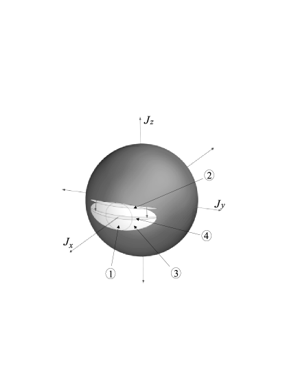
Figure 2: Schematic quasiprobability distributions for the spin state. The spin states are represented by ellipses on a sphere of radius $J$. The initial CSS, spin polarized in the $x$ direction is given by state 1. State 2 is one particular conditioned spin state after a measurement of $J_{z}$, while state 3 is the corresponding unconditioned state due to averaging over all possible conditioned states. The effect of the feedback is shown by state 4: A rotation about the $y$ axis shifts the conditioned state 2 back to $\left\langle{J_{z}}\right\rangle_{c}=0$. The ensemble average of these conditioned states will then be similar to state 4.

To make a rotation about the $y$ axis proportional to the measured photocurrent $I_{c}(t)$, we require a Hamiltonian of the form

$$H_{\rm fb}(t)=\hbar\lambda(t)I_{c}(t)J_{y}/\sqrt{M}=\hbar F(t)I_{c}(t),$$ (14)

where $F(t)=\lambda(t)J_{y}/\sqrt{M}$ and $\lambda(t)$ is the feedback strength. We have assumed instantaneous feedback because that is the form required to cancel Eq. (13). Such a Hamiltonian can be effected, for example, by applying either the combination of a static and an amplitude-controlled rf magnetic field [29], as shown in Fig. 1, or two-photon excitation by amplitude-controlled optical Raman fields. In either case, the amplitude of the driving field is controlled by the combined signal $\lambda(t)I_{c}(t)$ [see Fig. 1$(a)$].

The conditioned evolution of the system due to the feedback, Eq. (14), and measurement, Eq. (11), is given by [28]

$$\rho_{c}(t+dt)=e^{{\cal K}I_{c}(t)dt}\{\rho_{c}+M{\cal D}[J_{z}]\rho_{c}dt+\sqrt{M}dW(t){\cal H}[J_{z}]\rho_{c}\},$$ (15)

where ${\cal K}\rho\equiv-i[F(t),\rho]$. The feedback terms of this conditioned evolution lead to a shift in the mean $J_{z}$ by an amount equal to

$$d\left\langle{J_{z}}\right\rangle_{\rm fb} = -\lambda(t)dW(t)\left\langle{J_{x}}\right\rangle_{c}/\sqrt{M}-\lambda(t)^{2}dt\left\langle{J_{z}}\right\rangle_{c}/2M$$ (16)

$${}\,~{}~{}~{}~{}-\lambda(t)dt\left\langle{J_{x}J_{z}+J_{z}J_{x}}\right\rangle_{c}$$

$$\approx -\lambda(t)I_{c}(t)dt\left\langle{J_{x}}\right\rangle_{c}/\sqrt{M}.$$

As before the approximation assumes that $\left\langle{J_{z}}\right\rangle_{c}=0$ and also that the correlation between $J_{z}$ and $J_{x}$ is unchanged by the feedback. This is reasonable because it is initially zero due to the symmetry of the CSS and the conditioned states will remain symmetrical as shown in Fig. 2.

Since the idea is to produce $\left\langle{J_{z}}\right\rangle_{c}=0$ via the feedback, the approximations above and in Eq. (13) apply and we can find a feedback strength such that Eq. (13) is cancelled by Eq. (16). The required feedback strength for our scheme is thus

$$\lambda(t)=2M\left\langle{J_{z}^{2}}\right\rangle_{c}/\left\langle{J_{x}}\right\rangle_{c},$$ (17)

which is obviously dependent on conditioned averages. The feedback control, as expressed by Eqs. (14) and (17), is essentially a form of state-estimation based feedback and has similarities to the method of Doherty et al [30]. Although it appears that the feedback depends directly on the instantaneous measurement current $I_{c}(t)$, the strength of this feedback is determined by the conditioned state expectation values. The current only appears directly in $H_{\rm fb}$ because of the assumptions we make about the conditioned state.

Although Eq. (17) is the ideal form of the feedback strength required to produce $\left\langle{J_{z}}\right\rangle_{c}=0$, it may be not experimentally practical since it is dependent on conditioned expectation values. This requires classical processing of measurement signal in real time to continually obtain the best estimates of the system variables $J_{x}$ and $J_{z}^{2}$, which are then fedback to the system via Eq. (17) and the Hamiltonian (14). What would be preferable is a series of data points or ideally an equation for $\lambda(t)$ that can be stored in a signal generator, as shown in Fig. 1$(a)$, without having to do these side calculations during the feedback process.

Applying the Markovian theory of Sec. IVA in Ref. [28], we obtain the continuous QND measurement and feedback master equation for arbitrary $\lambda(t)$. It is given by

$$\dot{\rho}=M{\cal D}[J_{z}]\rho-i\lambda(t)[J_{y},J_{z}\rho+\rho J_{z}]+\frac{\lambda(t)^{2}}{M}{\cal D}[J_{y}]\rho.$$ (18)

The terms in this equation describe, respectively, the measurement back-action, the feedback driving, and the noise introduced by the feedback. The master equation can also be rewritten in Lindblad form [28]:

$$\dot{\rho}=-i\mbox{$\frac{1}{2}$}[c^{\dagger}F(t)+F(t)c,\rho]+{\cal D}[c-iF(t)]\rho\equiv{\cal L}\rho,$$ (19)

where the system operator $c=\sqrt{M}J_{z}$ and $F(t)=\lambda(t)J_{y}/\sqrt{M}$ as before. Note that these equations describe the exact unconditioned evolution of the atomic system where the feedback strength is arbitrarily defined by $\lambda(t)$. Equation (17) thus describes one particular feedback scheme.

To find an experimentally suitable expression for $\lambda(t)$ we first assume the feedback is successful in shifting the conditioned squeezed states to $\left\langle{J_{z}}\right\rangle_{c}=0$. This can be tested by looking at the purity, ${\rm Tr}[\rho^{2}]$, of the ensemble and conditioned states. Assuming perfect measurement, the conditioned spin state will remain in a pure state. Thus, if the ensemble average also has a high purity, it must comprise of nearly identical highly pure conditioned states. Solving the master equation, Eq. (18), we find that the unconditional state does have a purity very close to one (see the numerical results section for details), and we are justified in applying the approximations $\left\langle{J_{x}}\right\rangle_{c}\simeq\left\langle{J_{x}}\right\rangle$ and $\left\langle{J_{z}^{2}}\right\rangle_{c}\simeq\left\langle{J_{z}^{2}}\right\rangle$ for the feedback strength.

We can now proceed to find analytical expressions for $\left\langle{J_{x}}\right\rangle$ and $\left\langle{J_{z}^{2}}\right\rangle$ and hence $\lambda(t)$. To find an expression for $\left\langle{J_{x}}\right\rangle$ we note that its decrease from $J$ is due to the increase of $(\Delta J_{y})^{2}$ from $J/2$. The only contributions to this increase are due to the measurement, i.e., the first term in Eq. (18), since the feedback operator ($\propto J_{y}$) commutes with $J_{y}$. Now, for $\left\langle{\mathbf{J}}\right\rangle\sim\Or(J)$, the uncertainty in $J_{y}$ has not increased greatly and we can use the approximation $\left\langle{J_{x}}\right\rangle\approx J\left\langle{\cos(\Delta J_{y}/J)}\right\rangle\approx J\exp[{-\left\langle{J_{y}^{2}}\right\rangle/2J^{2}}]$. Here the first approximation assumes that the angle defining the extent of the spin state in the $xy$ plane is $\sim\Delta J_{y}/J$, which requires $J\gg 1$, and the second approximation assumes near Gaussian statistics for $J_{y}$.

To find an expression for $\left\langle{J_{z}^{2}}\right\rangle$ we use assume that, for $\left\langle{\mathbf{J}}\right\rangle\sim\Or(J)$, the atomic sample will approximately remain in a minimum uncertainty state. This is equivalent to assuming that the feedback, apart from maintaining $\left\langle{J_{z}}\right\rangle=0$, does not significantly alter the decreased variance of $J_{z}$ that was produced by the measurement. This gives $\left\langle{J_{z}^{2}}\right\rangle\approx J^{2}/4\left\langle{J_{y}^{2}}\right\rangle$, where we have also used $\left\langle{J_{x}}\right\rangle\approx J$. This last step is essentially a linear approximation represented by replacing $J_{x}$ with $J$ in the commutator $[J_{y},J_{z}]=iJ_{x}$. From $d_{t}\left\langle{J_{y}^{2}}\right\rangle\equiv{\rm Tr}[J_{y}^{2}\dot{\rho}]$ we obtain $\left\langle{J_{y}^{2}}\right\rangle\approx J^{2}Mt+J/2$, where the linear commutator has been used instead of the usual cyclic commutator.

Substituting the approximation for $\left\langle{J_{y}^{2}}\right\rangle$ into the expressions for $\left\langle{J_{x}}\right\rangle$ and $\left\langle{J_{z}^{2}}\right\rangle$ we obtain

$$\left\langle{J_{z}^{2}}\right\rangle \approx (4Mt+2/J)^{-1},$$ (20)

$$\left\langle{J_{x}}\right\rangle \approx J\exp(-Mt/2),$$ (21)

and hence for the feedback strength we have

$$\lambda(t)\approx Me^{Mt/2}(1+NMt)^{-1}.$$ (22)

So we now have a form of the feedback strength which can be applied experimentally. The question is - how well does it work?

We can analytically approximate the degree of squeezing produced by the particular feedback scheme represented by Eq. (22). For our model $({\mathbf{n}}_{1},{\mathbf{n}}_{2},{\mathbf{n}}_{3})=(z,x,y)$ and the squeezing parameter, Eq. (1), becomes

$$\xi^{2}_{z}=\frac{N\left\langle{J_{z}^{2}}\right\rangle}{\left\langle{J_{x}}\right\rangle^{2}}\simeq\frac{N\lambda(t)}{2M\left\langle{J_{x}}\right\rangle}\approx e^{Mt}(1+NMt)^{-1}.$$ (23)

This leads to a minimum at $t_{*}\approx 1/M$ of

$$\xi^{2}_{\rm min}\approx e/N,~{}~{}N\gg 1.$$ (24)

Thus, the minimum attainable squeezing parameter asymptotically approaches an inverse dependence on the sample size, i.e., the Heisenberg limit. This dependence is verified numerically in Sec. 3.4.

3.3 Effective nonlinear interaction

The quantum correlations of our scheme can be compared with those obtained via the different nonlinear Hamiltonians introduced earlier, Eqs. (2) and (3). This requires the effective nonlinear Hamiltonian for our measurement and feedback scheme. The master equation in Lindblad form, Eq. (19), is by definition separated into reversible (Hamiltonian) and irreversible (diffusive) terms. The nonlinear spin interactions produced in our scheme are thus given by the Hamiltonian

$$H=\mbox{$\frac{1}{2}$}(c^{\dagger}F(t)+F(t)c)=\mbox{$\frac{1}{2}$}\lambda(t)(J_{z}J_{y}+J_{y}J_{z}).$$ (25)

This is equivalent to the Hamiltonian $H_{2}$ if we note that, for an initial CSS with mean spin in the $z$ direction, Eq. (3) produces a squeezed state in the $xy$ plane [1]. Thus, the appropriate “two-axis countertwisting” to squeeze the $J_{z}$ variance of of an initial CSS with mean spin in the $x$ direction, has the form of Eq. (25). It is therefore not surprising that our scheme, since it has essentially the same nonlinear effect on the collective spin as $H_{2}$, also gives a $1/N$ dependence for the minimum attainable squeezing parameter.

The advantage of our scheme is that it does not rely on internal nonlinear spin interactions of the sample, such as those produced by collisions in a Bose-Einstein condensate. In addition to creating the squeezed state, these nonlinear interactions proceed to destroy the squeezing at later times. As opposed to internal spin interactions, which can not easily be “switched off”, the measurement laser and applied magnetic fields in our scheme can. This is simply represented by setting $M=0$ in our equations, which gives $\lambda(t)=0$ and therefore the master equation becomes $\dot{\rho}=0$. Thus, no further evolution of the atomic system (in the rotating frame) occurs, and the spin is essentially “frozen” in the squeezed state.

The exact timing for this procedure can be calculated prior to the run if all experimental parameters are known. For Heisenberg-limited squeezing the measurement and feedback should be applied continuously for a time $t_{*}=1/M$. On the other hand, if weaker squeezing is desired, the time is found by solving Eq. (23). For short times and $N\gg 1$ this becomes $t\sim 1/MN\xi^{2}$. In practice the limiting factor to squeezing will be the time for significant atom losses, as discussed in Sec. 3.5. In any case, the degree of spin squeezing can simply be controlled by varying the duration of the nonlinear interaction.

3.4 Numerical results

In this section we will justify the approximations leading up to Eq. (22), as well as verifying the $N^{-1}$ dependence of $\xi^{2}_{\rm min}$. Regardless of the approximations, which were only used to determine the experimentally suitable form of $\lambda(t)$, the numerical results of this section are exact for the given feedback scheme. By this we mean that the master equation (18) [or Eq. (19)] is solved exactly for a feedback strength determined by Eq. (22). This can be done, for example, by using the Matlab quantum optics toolbox [31].

The first approximation was that the conditioned averages could be replaced by ensemble averages. As stated earlier, this can be tested by looking at the purity of the unconditioned state due to the analytical $\lambda(t)$. By iteratively solving the master equation (18) while updating $\lambda(t)$ at each time step [using Eq. (22)], we find the time evolution of the purity ($=\Tr[\rho^{2}]$) and the expectation values ($\left\langle{A}\right\rangle=\Tr[A\rho]$). In this way the exact solution for the squeezing parameter,

$$\xi^{2}_{z}=N\left\langle{J_{z}^{2}}\right\rangle/\left\langle{J_{x}}\right\rangle^{2},$$ (26)

is also found.

The results of this simulation are shown in Fig. 3, where the purity is given by the central curve, the expectation values are given by curves A and B, and the squeezing parameter is given by curve C. We can clearly see that the purity remains near unity for the times of interest; at the numerical minimum of the squeezing parameter it equals $0.978$. This implies that the measurement and feedback scheme has worked to produce nearly identical conditioned states. As discussed in Sec. 3.2, this justifies the replacement of the conditioned averages of Eq. (17) with ensemble averages and also the further approximations to obtain Eq. (22).

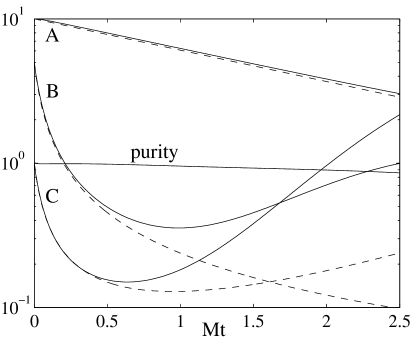
Figure 3: Time dependence of the purity $={\rm Tr}[\rho^{2}]$ (central curve), the expectation values $\left\langle{J_{x}}\right\rangle$ (A) and $\left\langle{J_{z}^{2}}\right\rangle$ (B), and the squeezing parameter $\xi^{2}_{z}$ (C) for $N=20$. The solid lines represent the exact numerical solutions of the master equation with Eq. (22) for the feedback strength. The dashed lines are the corresponding analytical expressions given by Eqs. (20), (21) and (23).

The analytical expressions for the expectation values, Eqs. (20) and (21), and the squeezing parameter, Eq. (23), are also included in Fig. 3 (dashed lines). As can be seen the analytical approximation (dashed curve A) for $\left\langle{J_{x}}\right\rangle$ is quite good, while the approximation (dashed curve B) for $\left\langle{J_{z}^{2}}\right\rangle$ is only good for times up to the $\xi_{z}^{2}$ minimum. Since we are only interested in applying the scheme up until this point, this is acceptable. As a result though, the analytical minimum for the squeezing parameter is not a perfect fit to the exact numerical results. However, it is the correct order of magnitude and so we expect the analytical scaling predicted by Eq. (24), i.e. $N^{-1}$, to be correct.

To reiterate, the analytical equation (22) for the feedback strength succeeds in maintaining the conditional squeezing (produced by the measurement) in a constant mean spin direction (hence the high values for the purity of the ensemble average state). It is also of a suitable form for experimental realization. We now proceed to study the limit to the squeezing produced by this scheme. In Fig. 4 the squeezing parameter is plotted for three different sample sizes. The dotted line refers to the case of no measurement and no feedback. As can be seen, the squeezing becomes stronger as the number of atoms in the sample is increased.

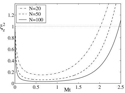
Figure 4: Typical time dependence of the squeezing parameter $\xi^{2}_{z}$ for the continuous measurement and feedback scheme for three different sample sizes $N=20$, $N=50$, and $N=100$. The dotted line represents no measurement and no feedback, i.e., the sample remains in the CSS.

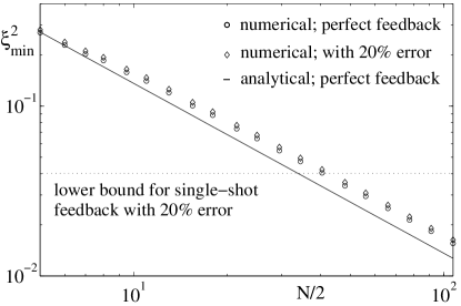
Figure 5: Atom number dependence of the squeezing parameter minimum, $\xi^{2}_{\rm min}$. This figure presents the results of numerical solutions of the ME, and hence Eq. (26), with $\lambda(t)$ given by Eq. (22) (circles) and $\lambda(t)\times 120\%$ (diamonds). These values approach $3.33/N$ and $3.49/N$ respectively. The dotted line is the lower-bound for single-shot feedback also with a $20\%$ error, while the analytical result for perfect continuous feedback $e/N$, Eq. (24), is the solid line.

To find how the minimum of $\xi^{2}_{z}$ scales with increasing sample size, we extract $\xi^{2}_{\rm min}$ numerically from the above simulation. The minimum attainable squeezing parameter approaches an inverse dependence on $N$ as the sample size increases, as shown in Fig. 5. In this figure, the analytical result for $\xi^{2}_{\rm min}$, given by Eq. (24), is plotted along with the minima obtained from the numerical simulation. The analytical coefficient ($e\approx 2.72$) represents an error of $\sim 18\%$ compared to the numerical fit ($3.33/N$), which is to be expected from Fig. 3. Nevertheless, these errors only apply to scaling coefficients, not to the scalings themselves. Thus, for our continuous measurement and feedback scheme, we can conclude that the minimum attainable squeezing parameter scales as $N^{-1}$ and occurs after a time of the order of $M^{-1}$. The exact values for a given sample size can be obtained by numerical simulation.

3.5 Experimental considerations

Our continuous scheme, as opposed to a single-shot method, is very robust to any experimental errors in the feedback strength, as is shown in Fig. 5. The latter approach consists of a single (integrated) measurement pulse (see e.g., [17]), followed by a single feedback pulse. If there is a relative error of $\epsilon$ in the feedback strength, this will induce an error term $(\Delta J_{z}^{\rm err})^{2}\sim\epsilon^{2}N/4$, which will dominate the total variance for $N\gg 1$. Thus $\xi^{2}_{\rm min}$ will have a lower bound of $\epsilon^{2}$, and will never scale as $N^{-1}$. On the other hand, as shown in Fig. 5, a large ($20\%$) error in $\lambda(t)$ for continuous feedback does not affect the $N^{-1}$ scaling.

Although the analysis presented in this paper is based on instantaneous feedback (in order to determine analytically the limit to squeezing), including a finite delay time will have a limited effect as long as it is of the order of $\tau_{\rm fb}\sim(NM)^{-1}$. This is the fastest timescale in the equation (22) for the feedback strength, and we discuss below the implications this time has for practical application. Furthermore, we have found the theoretical $N^{-1}$ scaling of the squeezing parameter, $\xi_{z}^{2}$, to be unaffected by inefficient measurements. This is detailed in the Appendix.

Experimentally, the limit to squeezing will most likely be dominated by spontaneous atom losses due to absorption (and hence scattering) of QND probe light. For a detailed study of the effects of photon scattering in optical phase-shift measurements see the recent work by Bouchoule and Mølmer [32]. Since the scattered photons carry information about the atoms that is not recorded, this process can also be treated in the same way as detector inefficiency (a discussion of this is presented in the Appendix, where we show similar scalings for $\xi^{2}_{\rm min}$ to that of Ref. [32]).

In the present discussion we take the more extreme approach of looking at atom losses from the spin-$J$ system due to absorption of the probe light. In this way we estimate the limiting values of the spin squeezing parameter for both cavity and free space situations. From Eq. (4) it can be seen that the single atom loss rate in the far-detuned limit will be $\Gamma=\gamma\Omega^{2}/4\Delta^{2}$, where $\gamma$ is the spontaneous emission rate, $\Omega$ is the Rabi frequency and $\Delta$ the detuning. For the cavity field interaction, $\Omega^{2}=g^{2}|\beta|^{2}$, $M=8\chi^{2}P/\hbar\omega\kappa^{2}$ and $\chi=g^{2}/4\Delta$, and so $\Gamma=\kappa\gamma M/g^{2}$. For the free space model, $\Omega^{2}=\gamma^{2}I/2I_{\rm sat}$, $P=IA$, and $M=P\theta^{2}/\hbar\omega$ where $\theta$ and $I_{\rm sat}$ are defined before Eq. (8), and so we obtain $\Gamma=16\pi^{2}AM/\lambda^{2}$. The single atom loss rate can therefore be expressed in general as

$$\Gamma=\alpha M,$$ (27)

where $\alpha=\kappa\gamma/g^{2}$ for the cavity and $16\pi^{2}A/\lambda^{2}$ for free space, and so the number of atoms lost by time $t$ can be estimated by

$$\Delta N=\Gamma Nt=\alpha MNt.$$ (28)

Therefore, by the time ($\sim 1/M$) to reach the Heisenberg limit we have lost $\Delta N\sim\alpha N$ atoms. From Sec. 3.3, the time to reach an arbitrary amount of squeezing is $t\sim 1/NM\xi^{2}$, so we can say that the total number of atoms lost scales as $\Delta N\sim\alpha/\xi^{2}$.

Determining the maximum number of atoms that can be lost before destroying a given value of squeezing will thus give us some realistic constraints that should be placed on $\alpha$. Recently, André and Lukin analyzed the squeezing produced by the counter-twisting Hamiltonian, Eq. (3), including the effects of dissipation [34]. They showed that for a given amount of spin squeezing $\xi^{2}=1/s$, where $1<s\leq N$, the maximum number of atoms that can be lost without destroying the squeezing scales as $\Delta N_{\rm max}\sim(N/s)\ln s$ [34]. In other words, to achieve the desired level of squeezing, we need to set $\Delta N\sim\Delta N_{\rm max}$. This becomes $\alpha/\xi^{2}\sim N\xi^{2}\ln(1/\xi^{2})$. Given an arbitrary $\alpha$, the amount of squeezing produced including atom losses therefore scales as

$$\xi^{2}\sim\sqrt{\alpha/N}.$$ (29)

So to produce any squeezing we need $\alpha<N$, for $\xi^{2}\sim 1/\sqrt{N}$ we need $\alpha\sim 1$, and for the Heisenberg limit we need $\alpha\sim 1/N$.

For the case of the cavity field interaction, $\alpha=\kappa\gamma/g^{2}$, so the requirement for Heisenberg limited squeezing becomes $g^{2}\sim N\kappa\gamma$. This can only be fulfilled in the very strong coupling regime, which, although difficult, has been achieved experimentally [33]. Looking at the other regimes, we find that $\xi^{2}\sim 1/\sqrt{N}$ squeezing will be observed for $g^{2}\sim\kappa\gamma$, and the generation of any squeezing, i.e., $\xi^{2}<1$, will be observed for $g^{2}N>\kappa\gamma$. These are the same results as found in Ref. [34]. As might be expected, the free space model will not reach the Heisenberg limit. In this case $\alpha=16\pi^{2}A/\lambda^{2}$, so the requirement becomes $A\sim\lambda^{2}/16\pi^{2}N$ which is not possible. The limiting value for squeezing in this case would be near $1/\sqrt{N}$, since this would be produced if $A\sim\lambda^{2}/16\pi^{2}$, and to achieve any squeezing we only require $A<N\lambda^{2}/16\pi^{2}$. So for the free space regime we still expect a significant amount of squeezing to be possible.

We can also determine the constraints that need to be placed on the probe laser by recognizing that our analysis is based on a far-detuned optical probe with $\Delta\gg\Omega$. This implies that $\Gamma\ll\gamma$, and thus from Eq. (27), $M\ll\gamma/\alpha$. The measurement strength for both schemes can be re-expressed as

$$M=\gamma^{2}P/\hbar\omega\Delta^{2}\alpha^{2},$$ (30)

and hence our laser requirements are

$$P/\Delta^{2}\ll\hbar\omega\alpha/\gamma.$$ (31)

Take for example $N=10^{7}$ Cesium atoms, where $\lambda=852$ nm ($\omega/2\pi=352$ THz) and $\gamma=5$ MHz. Then to obtain spin squeezing in either the free space or cavity regimes, we only need $P\ll 10^{-18}\Delta^{2}$. On the other hand, to reach Heisenberg limited squeezing ($\alpha\sim 1/N$) we have the added requirement that $P\ll 10^{-33}\Delta^{2}$ as well as strong cavity coupling. Looking at a detuning of $\Delta=1$ GHz, this restricts the laser power to femtoWatts, which should be possible [35].

Finally, realistic feedback delay times will give some additional restrictions on the possible squeezing. As mentioned earlier, the feedback needs to act on a timescale of order $1/NM$, which becomes $\tau_{\rm fb}\sim\hbar\omega\Delta^{2}\alpha^{2}/NP\gamma^{2}$ using the general expression for $M$. For $P=1$ fW and $\Delta=1$ GHz, this time is of the order $10\alpha^{2}/N$ s. Typical feedback delay times are of order $10^{-7}$ s [35], so unless the number of atoms is restricted to a few hundred, the Heisenberg limit (where $\alpha\sim 1/N$) will not be feasible.

During the preparation of this paper we became aware of an analysis of the entanglement in bad cavities by Sørensen and Mølmer [36]. Although the scheme described in that work is very different from ours (in fact it is similar to Ref. [34]), it also reaches similar results. All three schemes require very strong cavity couplings to produce Heisenberg limited squeezing, but weaker (and perhaps more useful) squeezing can be produced in bad cavities and free space.

4 Conclusion

In conclusion we have detailed a scheme for achieving, and controlling, the spin squeezing of an atomic sample by a continuous quantum feedback mechanism using an optical probe. This scheme has the advantage over previous schemes involving QND measurement [15, 16] in that it produces unconditional, or deterministically reproducible, squeezing. This means that the same squeezed spin state, which is also an entangled state [5, 6], will be produced regardless of the particular measurement record. It is therefore a more practical state for use in quantum information.

The theoretical squeezing (or entanglement) parameter approaches the Heisenberg limit of $\xi^{2}\sim 1/N$ for very strong cavity couplings, a limited number of atoms, very large detuning and small laser power. This $1/N$ scaling indicates a stronger squeezing mechanism than collisional interactions in a Bose-Einstein condensate where the scaling is $N^{-2/3}$ [5, 9]. By ceasing the measurement and feedback interactions when the desired squeezing parameter has been reached, the squeezed state could be maintained indefinitely. Thus, once this state is generated, there will be no further decoherence due to the interactions of its production.

Significant squeezing will still be produced at weaker cavity couplings, and even in free space, with correspondingly less stringent experimental requirements. The free space QND measurement regime therefore presents a relatively simple, and interesting, experimental implementation of quantum feedback, an area which is still in its infancy. Also, the weaker the squeezing the less vulnerable the state is to further decoherence after its production. The Heisenberg-limited squeezed state will be severely affected by the loss of a few atoms, whereas less strongly squeezed states can lose many without serious damage [34]. The states produced in a free space scheme might therefore be adequate for practical quantum information, where other experimental factors could destroy the more sensitive states. Then, if necessary, one can devise entanglement purification procedures for atomic samples [37]. Finally, achieving and controlling a spin squeezed state could also be useful in obtaining tomographic phase space pictures of nonclassical states of atomic samples [38].

Appendix A Inefficient measurements

In real experiments there is a finite efficiency involved in the measurement process. We now include this in our analysis to see whether the degree of spin squeezing is significantly affected. Basically, only a certain proportion ($\eta$) of the probe beam is actually detected and then used for feedback, but the undetected proportion ($1-\eta$) still causes back-action on the system. This could be due to only monitoring the output of one side of a cavity [as in Fig. 1$(a)$], or imperfect photodetectors, or even undetected photons scattered off the atomic sample (which is treated more rigorously in Ref. [32]).

Let us first look at the effect of an inefficient measurement of $J_{z}$, before adding the feedback. The stochastic master equation $d\rho_{c}$ is now made up of two contributions: the actual homodyne detection of a proportion $\eta$ of the probe light

$$\eta{\cal D}[c]\rho_{c}dt+\sqrt{\eta}dW(t){\cal H}[c]\rho_{c},$$ (32)

plus the back-action due to the probe light that wasn’t detected

$$(1-\eta){\cal D}[c]\rho_{c}dt,$$ (33)

where $c=\sqrt{M}J_{z}$ as before. Similarly, the homodyne photocurrent is now given by

$$I_{c}(t)=\eta\left\langle{c+c^{\dagger}}\right\rangle_{c}+\sqrt{\eta}\xi(t).$$ (34)

The stochastic shift in $\left\langle{J_{z}}\right\rangle_{c}$ due to an inefficient measurement is therefore $2\sqrt{\eta M}dW(t)(\Delta J_{z})^{2}_{c}$. If we again assume $\left\langle{J_{z}}\right\rangle_{c}\approx 0$ (which will be true when the feedback is included) then $I_{c}(t)\approx\sqrt{\eta}dW/dt$ and so we again obtain the approximation in Eq. (13).

Including feedback to cancel this stochastic shift, we obtain the same feedback Hamiltonian (14) as before, although note that the current $I_{c}(t)$ is now defined by Eq. (34). Thus, the shift in the mean $J_{z}$ due to feedback is still given by Eq. (16) and the optimal feedback strength is therefore also unchanged from the form given in Eq. (17). It is the assumptions made for obtaining the analytical expression for $\lambda(t)$ that are now complicated.

The master equation for the inefficient measurement and feedback is given by

$$\dot{\rho}=(1-\eta+\eta){\cal D}[c]\rho-i[F,c\rho+\rho c^{\dagger}]+\frac{1}{\eta}{\cal D}[F]\rho,$$ (35)

where $c=\sqrt{M}J_{z}$ and $F=\lambda(t)J_{y}/\sqrt{M}$ as before. Thus, the total back-action due to the probe does not depend on the detection efficiency since it is made up of both the detected ($\eta$) and undetected ($1-\eta$) contributions. The Lindblad form of the master equation, Eq. (19), now also has the additional term $[(1-\eta)/\eta]{\cal D}[F]\rho$.

To simplify the form of $\lambda(t)$ in Eq. (17) we again assume the feedback is successful and replace the conditioned averages with ensemble averages. To find $\left\langle{J_{z}^{2}}\right\rangle$ we earlier assumed a near minimum uncertainty state, but this cannot be true for imperfect measurements. To use $\left\langle{J_{z}^{2}}\right\rangle\approx J^{2}/4\left\langle{J_{y}^{2}}\right\rangle$ for $\eta<1$ we must therefore calculate the average $J_{y}^{2}$ only using the evolution due to the actual measurement and feedback, i.e. we ignore $(1-\eta){\cal D}[c]\rho$. This gives $\left\langle{J_{y}^{2}}\right\rangle\approx J^{2}\eta Mt+J/2$ and then $\left\langle{J_{z}^{2}}\right\rangle\approx(4\eta Mt+2/J)^{-1}$. To find $\left\langle{J_{x}}\right\rangle$ we earlier noted that it decreased indirectly due to the measurement back-action. As shown above, the total back-action due to the probe beam is independent of detection efficiency and so we can keep the earlier approximation (21) for $\left\langle{J_{x}}\right\rangle$.

These approximations for the averages this time lead to a feedback strength of

$$\lambda(t)\approx Me^{Mt/2}(1+\eta NMt)^{-1}.$$ (36)

The approximate squeezing parameter then becomes

$$\xi^{2}_{z}\approx e^{Mt}(1+\eta NMt)^{-1},$$ (37)

which has a minimum at $t_{*}\approx 1/\eta M$ of

$$\xi^{2}_{\rm min}\approx e^{1/\eta}/N,~{}~{}N\gg 1.$$ (38)

So for $\eta<1$, the minimum attainable squeezing parameter is greater than that for $\eta=1$. However, finite efficiency only affects the coefficient of this minimum - the $N^{-1}$ dependence is unaffected. Note that this is the same scaling with the number of atoms as found in Eq. (59) of Ref. [32], which confirms that photon scattering can also be regarded as a measurement inefficiency.

References

References

- [1] M. Kitagawa and M. Ueda, Phys. Prev. A 47, 5138 (1993).
- [2] Special issue on Quantum Information, Phys. World 11, 33 (1998).
- [3] D. J. Wineland, J. J. Bollinger, W. M. Itano, and D. J. Heinzen, Phys. Rev. A 46, R6797 (1992); D. J. Wineland, J. J. Bollinger, W. M. Itano, F. L. Moore, and D. J. Heinzen, Phys. Rev. A 50, 67 (1994); P. Bouyer and M. Kasevich, Phys. Rev. A 56, R1083 (1997).
- [4] J. S. Bell, Speakable and Unspeakable in Quantum Mechanics (Cambridge University Press, 1988).
- [5] A. Sørensen, L.-M. Duan, J. I. Cirac, and P. Zoller, Nature 409, 63 (2001).
- [6] A. Sørensen and K. Mølmer, Phys. Rev. Lett. 86, 4431 (2001).
- [7] A. Kuzmich, K. Mølmer, and E. S. Polzik, Phys. Rev. Lett. 79, 4782 (1997); E. S. Polzik, Phys. Rev. A 59, 4202 (1999); A. E. Kozhekin, K. Mølmer, and E. S. Polzik, Phys. Rev. A 62, 033809 (2000).
- [8] J. Hald, J. L. Sørensen, C. Schori, and E. S. Polzik, Phys. Rev. Lett. 83, 1319 (1999).
- [9] C. K. Law, H. T. Ng, and P. T. Leung, Phys. Rev. A 63, 055601 (2000); U. V. Poulsen and K. Mølmer, Phys. Rev. A 64, 013616 (2001); A. Sørensen, cond-mat/00110372.
- [10] H. Pu and P. Meystre, Phys. Rev. Lett. 85, 3987 (2000); L.-M. Duan, A. Sørensen, J. I. Cirac, and P. Zoller, Phys. Rev. Lett. 85, 3991 (2000).
- [11] K. Mølmer and A. Sørensen, Phys. Rev. Lett. 82, 1835 (1999).
- [12] K. Helmerson and L. You, Phys. Rev. Lett. 87, 170402 (2001).
- [13] U. V. Poulsen and K. Mølmer, Phys. Rev. A 63, 023604 (2001).
- [14] C. Orzel, A. K. Tuchman, M. L. Fenselau, M. Yasuda, and M. A. Kasevich, Science 291, 2386 (2001).
- [15] A. Kuzmich, N. P. Bigelow, and L. Mandel, Europhys. Lett. 42, 481 (1998).
- [16] A. Kuzmich, L. Mandel, and N. P. Bigelow, Phys. Rev. Lett. 85, 1594 (2000).
- [17] L.-M. Duan, J. I. Cirac, P. Zoller, and E. S. Polzik, Phys. Rev. Lett. 85 5643 (2000).
- [18] B. Julsgaard, A. Kozhekin, and E. S. Polzik, Nature 413, 400 (2001).
- [19] L. K. Thomsen, S. Mancini, and H. M. Wiseman, Phys. Rev. A 65, 061801(R) (2002).
- [20] H. M. Wiseman and G. J. Milburn, Phys. Rev. A 49, 1350 (1994).
- [21] K. Mølmer, Eur. Phys. J. D 5, 301 (1999).
- [22] R. H. Dicke, Phys. Rev. 93, 99 (1954).
- [23] M. R. Andrews, M.-O. Mewes, N. J. van Druten, D. S. Durfee, D. M. Kurn, and W. Ketterle, Science 273, 84 (1996).
- [24] X. Wang, J. Opt. B: Q. Semiclass. Opt. 3, 93 (2001); X. Wang, quant-ph/0109125.
- [25] J. F. Corney and G. J. Milburn, Phys. Rev. A 58, 2399 (1998).
- [26] L. K. Thomsen and H. M. Wiseman, Phys. Rev. A 56, 063607 (2002).
- [27] A. Ashkin, Phys. Rev. Lett. 25, 1321 (1970).
- [28] H. M. Wiseman, Phys. Rev. A 49, 2133 (1994); 49, 5159(E) (1994); 50, 4428(E) (1994).
- [29] R. T. Sang, G. S. Summy, B. T. H. Varcoe, W. R. MacGillivray, and M. C. Standage, Phys. Rev. A 63, 023408 (2001).
- [30] A. C. Doherty, S. Habib, K. Jacobs, H. Mabuchi, and S. M. Tan, Phys. Rev. A 62, 012105 (2000).
- [31] S. M. Tan, J. Opt. B: Q. Semiclass. Opt. 1, 424 (1999).
- [32] I. Bouchoule and Klaus Mølmer, quant-ph/0205082.
- [33] P. W. H. Pinkse et al., J. Mod. Opt. 47, 2769 (2000); C. J. Hood et al., Phys. Rev. A 64, 033804 (2001).
- [34] A. Andre and M. D. Lukin, Phys. Rev. A 65, 053819 (2002).
- [35] M. A. Armen, J. K. Au, J. K. Stockton, A. C. Doherty, and Hideo Mabuchi, quant-ph/0204005.
- [36] A. S. Sørensen and K. Mølmer, quant-ph/0202073.
- [37] J. A. Dunningham, S. Bose, L. Henderson, V. Vedral, and K. Burnett, Phys. Rev. A 65, 064302 (2002).
- [38] S. Mancini and P. Tombesi, Europhys. Lett. 40, 351 (1997); E. L. Bolda, S. M. Tan, and D. F. Walls, Phys. Rev. Lett. 79, 4719 (1998); R. Walser, Phys. Rev. Lett. 79, 4724 (1998); E. L. Bolda, S. M. Tan, and D. F. Walls, Phys. Rev. A 57, 4686 (1998); S. Mancini, M. Fortunato, P. Tombesi and G. M. D’Ariano, J. Opt. Soc. Am. A 17, 2529 (2000).