Conditional phase shifts using trapped atoms

Abstract

We describe a scheme for producing conditional nonlinear phase shifts on two-photon optical fields using an interaction with one or more ancilla two-level atomic systems. The conditional field state transformations are induced by using high efficiency fluorescence shelving measurements on the atomic ancilla. The scheme can be nearly deterministic and is of obvious benefit for quantum information applications.

It has recently been shown KLM that nonlinear phase shifts on two photon states can be produced by coupling the mode of interest to ancilla modes via a beam splitter and making photon counting measurements on the ancilla modes. Such conditional nonlinear phase shifts can be used to perform two qubit operations for logical states encoded in photon number states. If such conditional gates are used to prepare entangled states for teleportation, efficient quantum computation can be performed which with suitable error correcting codes can be made fault tolerant KLM . In this paper we show that if the ancilla modes are replaced with a two level atom similar conditional nonlinear phase shifts can be achieved by near deterministic postslection on atomic measurements. The atomic measurements can made with fluorescence shelving techniques which are very much more efficient than single photon counting measurements, thus reducing the need for new photon counting technologies inherent in the KLM scheme. Recently, a different scheme for conditional quantum gates based on atomic systems was presneted by Protsenko et al.protsenko

Consider a single optical mode prepared in an arbitrary two photon state

$$|\psi\rangle=c_{0}|0\rangle+c_{1}|1\rangle+c_{2}|2\rangle$$ (1)

Our objective is to find a way to produce the nonlinear phase shift transformation defined by

$$|\psi\rangle\rightarrow c_{0}|0\rangle+c_{1}|1\rangle-c_{2}|2\rangle$$ (2)

To achieve this result we assume that at some fixed time an interaction between the field mode and a single two level atom is switched on. After some interaction time $t$ the interaction is turned off and the atomic state is measured by fluorescence shelving. The resulting conditional state of the field will then depend on the initial state of the two-level atom and the interaction time. We will show that these can be so arranged as to effect the nonlinear phase shift required.

We have in mind a quantum computing communication protocol in which the optical field mode is derived from a transform limited pulsed field which is rapidly switched into the cavity mode containing the atomic systems at fixed times determined by the pulse repetition rate. Similar systems have been proposed as a quantum memory for optical information processing Pittman2002 . When the atomic measurement yields the required result the field may be switched out again for further analysis or subsequent processing through linear and conditional elements.

Once the cavity field is prepared, we need to switch on the interaction with the atomic system. In order that we can switch this interaction at predetermined times we propose that an effective two level transition connected by a Raman process with one classical field and the quantised signal field, be used. A similar scheme has recently been proposed as the basis of a high efficiency photon counting measurement Imamoglu ; James_Kwiat . The process is also used in the EIT schemes for storing photonic information Lukin2000 and for quantum state transfer between distant cavities Cirac1997 . The level diagram is shown in figure 1. The nearly degenerate levels $|1\rangle$ and $|2\rangle$ are connected by a stimulated Raman transition to level $|3\rangle$. The detuning of the Raman pulse from the excited state $|3\rangle$ is $\Delta$, which is approximately the same as the detuning of the signal mode form the same transition. An advantage of using a stimulated Raman process of this kind is that the excited state $|2\rangle$ can be a metastable, long lived level. We thus do not need to consider spontaneous emission from this level back to the ground state. The readout of the atomic system may be achieved by using a cycling transition between the excited state $|2\rangle$ and another probe level $|4\rangle$. Such measurements are routinely performed in ion trap studies Rowe2000 and can have efficiencies greater than 99%.

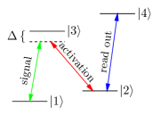
Figure 1: Level scheme for an effective two-level transition controlled by a stimulated Raman process.

The interaction between the single mode field and a two-level atom is described by the effective Hamiltonian

$$\mbox{\boldmath$\hat{H}$}=\kappa(\mbox{\boldmath$\hat{a}$}^{\dagger}\mbox{\boldmath$\hat{\sigma}$}^{-}+\mbox{\boldmath$\hat{a}$}\mbox{\boldmath$\hat{\sigma}$}^{+})$$ (3)

The interaction strength is given by $\kappa=\Omega g/2\Delta$ where $\Omega$ is the Rabi frequency for the Raman pulse and $g$ is the one photon Rabi frequency for the signal field. The unitary transformation that acts when this interaction is applied for a time $t$ is

$$\mbox{\boldmath$\hat{U}$}(\tau)=\exp[-i\tau(\mbox{\boldmath$\hat{a}$}^{\dagger}\mbox{\boldmath$\hat{\sigma}$}^{-}+\mbox{\boldmath$\hat{a}$}\mbox{\boldmath$\hat{\sigma}$}^{+})]$$ (4)

where $\tau=\kappa t$.

If the atom is prepared in the ground state and found in the ground state after the interaction, the conditional state of the field is given by

$$\mbox{\boldmath$\hat{\Upsilon}$}_{gg}(\tau)\mbox{$|\psi\rangle$}=\cos(\tau\sqrt{\mbox{\boldmath$\hat{a}$}^{\dagger}\mbox{\boldmath$\hat{a}$}})\mbox{$|\psi\rangle$}$$ (5)

On the other hand if the atom is prepared in the exited state and found in the excited state after the interaction, the conditional state is given by

$$\mbox{\boldmath$\hat{\Upsilon}$}_{ee}(\tau)\mbox{$|\psi\rangle$}=\cos(\tau\sqrt{\mbox{\boldmath$\hat{a}$}\mbox{\boldmath$\hat{a}$}^{\dagger}})\mbox{$|\psi\rangle$}$$ (6)

There is considerable practical advantage to using the excited state preparation rather than the ground state as there is always a signal for correct operation, however the analysis is the same.

Now suppose we send in a generic two photon state

$$\mbox{$|\psi\rangle$}=c_{0}\mbox{$|0\rangle$}+c_{1}\mbox{$|1\rangle$}+c_{2}\mbox{$|2\rangle$}$$ (7)

which interacts with a single two level atom, prepared in the ground state, and after the interaction the atom is found still to be in the ground state. In this case we need to apply the measurement operator $\mbox{\boldmath$\hat{\Upsilon}$}_{gg}$, and the resulting state of the field is

$$\mbox{$|\phi_{g}\rangle$}=A_{0}c_{0}\mbox{$|0\rangle$}+A_{1}c_{1}\mbox{$|1\rangle$}+A_{2}c_{2}\mbox{$|2\rangle$}$$ (8)

where $A_{0}=1$, $A_{1}=\cos(\tau)$ and $A_{2}=\cos(\sqrt{2}\tau)$. Note that the frequencies of the $A_{1}$ and $A_{2}$ terms are irrational multiples of each other. As we sweep $\tau$, $A_{1}$ and $A_{2}$ should explore their entire phase space. It should be possible to find values of $\tau$ for which $(A_{1},A_{2})$ approaches arbitrarily close to $(1,-1)$. These solutions can be found trivially for small $\tau$ by plotting $A_{1}$ and $-A_{2}$ and visually inspecting for intersections near 1. Some high-probability solutions are summarised in table 1.

$\tau$	$A_{0}$	$A_{1}$	$A_{2}$
6.5064	1	0.97519	-0.97516
37.73742	1	0.9992663	-0.9992665
219.918	1	0.999979	-0.999978

Table 1: High-probability results for a single atom initially in a ground state and measured in a ground state after an interaction time $\tau$.

With two atoms, one initially prepared in the ground state and the second prepared in the excited state, the conditional state given that both atoms are found in their initial state after the interaction is

$$|\phi_{ge}\rangle = \mbox{\boldmath$\hat{\Upsilon}$}_{gg}(\tau_{1})\mbox{\boldmath$\hat{\Upsilon}$}_{ee}(\tau_{2})\mbox{$|\psi\rangle$}$$ (9)

$$= A_{0}c_{0}\mbox{$|0\rangle$}+A_{1}c_{1}\mbox{$|1\rangle$}+A_{2}c_{2}\mbox{$|2\rangle$}$$ (10)

where $A_{0}=\cos(\tau_{2})$, $A_{1}=\cos(\tau_{1})\cos(\sqrt{2}\tau_{2})$ , and $A_{2}=\cos(\sqrt{2}\tau_{1})\cos(\sqrt{3}\tau_{2})$.

By using two atoms, each with a different interaction time, we have more freedom in locating solutions for which the magnitude of the $A_{i}$’s are closer together. This occurs at the expense of a more complex experimental scheme. To find solutions we employed a simulated annealing algorithm on an initial ensemble of randomly chosen points. After the points where suitably ‘cooled’ relative to a penalty function, we applied a simplex minimisation method on the top contenders to find the local minima. Some interaction times that result in implementing nearly ideal nonlinear-sign gates with high probability are given in table 2.

$\tau_{1},\tau_{2}$	$A_{0}$	$A_{1}$	$A_{2}$
477.60911391, 197.78326606	-0.9906204535	-0.9906204532	+0.9906204537
37.79300921, 197.78109842	-0.9903219354	-0.9903219357	+0.9903219350

Table 2: High-probability results for two atoms, one initially in a ground state the other in an exited state and detected in their initial states after interaction times $\tau_{1}$ and $\tau_{2}$.

In an experiment it would be necessary to find a way to calibrate the interaction time until the desired phase shift had been reached. One way to do this is depicted in figure 2. Two single modes, each prepared in a one photon state are incident on a 50/50 beam splitter. The two photon interference then results in the state $|2\rangle|0\rangle-|0\rangle|2\rangle$. The conditional phase shift can then be inserted on one arm so that the state is transformed to $|2\rangle|0\rangle-e^{i\theta}|0\rangle|2\rangle$. This state is then run through an identical 50/50 beam splitter to the first and the probability for coincidence counts is sampled. This probability is given by $P_{c}=\cos^{2}\theta/2$. The coincidence detection rate then drops to zero at the required conditional phase shift of $\theta=\pi$.

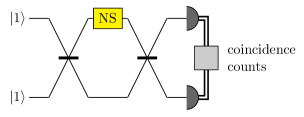
Figure 2: An interferometric scheme for calibrating the conditional nonlinear sign shift gate (NS) by searching for coincidence counts from the photon detectors (PD).

We now estimate some typical values for the parameters. In a recent experiment a similar stimulated Raman process was observed using single rubidium atoms falling through a high finesse optical cavity Henrich2000 . The following parameters are typical of that experiment: $g=2\pi\times 4.5$ MHz, $\Omega=2\pi\times 30$ MHz and $\Delta=2\pi\times 6$ MHz. This gives a coupling constant of the order of $70$ Mhz. To achieve effective interaction constants of the order of those in the table 1 requires interaction times of the order of $0.1-5$ $\mu$s. In this paper we have neglected cavity decay which obviously needs to be kept small over similar time scale, which while difficult is not impossible.

We would like to thank the Computer Science department of the University of Waikato for making available their computing resources. AG was supported by the New Zealand Foundation for Research, Science and Technology under grant UQSL0001. GJM was supported by the Cambridge-MIT Institute while a visitor at University of Cambridge.

References

- (1) E. Knill, R. Laflamme and G.J. Milburn, Nature,409, 46 (2001).
- (2) I.E.Protsenko, G.Reymond, N. Schlosser and P.Grangier, quant-ph/0206007 (2002) .
- (3) A. Imamoglu,arXiv:quant-ph/0205196 (2002).
- (4) D.F. James and P.G. Kwiat arXiv:quant-ph/0206049 (2002).
- (5) M. Fleischhauer and M.D. Lukin, Phys. Rev. Letts. 84, 5094, (2000).
- (6) J.I. Cirac, P. Zoller, H.J. Kimble and M. Mabuchi, Phys. Rev. Letts. 78, 3221 91997).
- (7) T.B. Pittman and J.D. Franson, arXiv:quant-ph/0207041 (2002).
- (8) M.A. Rowe et al., Nature, 409, 791 (2000).
- (9) M. Henrich, T. Legero, A. Kuhn and G. Rempe, Phys. Rev. Letts. 85, 4872 (2000).