Quantum computation with unknown parameters

Abstract

We show how it is possible to realize quantum computations on a system in which most of the parameters are practically unknown. We illustrate our results with a novel implementation of a quantum computer by means of bosonic atoms in an optical lattice. In particular we show how a universal set of gates can be carried out even if the number of atoms per site is uncertain.

Scalable quantum computation requires the implementation of quantum gates with a very high fidelity. This implies that the parameters describing the physical system on which the gates are performed have to be controlled with a very high precision, something which it is very hard to achieve in practice. In fact, in several systems only very few parameters can be very well controlled, whereas other posses larger uncertainties. These uncertainties may prevent current experiments from reaching the threshold of fault tolerant quantum computation (i.e. gate fidelities of the order of $0.9999$ tolerancia ), that is, the possibility of building a scalable quantum computer. For example, in quantum computers based on trapped ions or neutral atoms cold-atoms , the relative phase of the lasers driving a Raman transition can be controlled very precisely, whereas the corresponding Rabi frequency $\Omega$ has a larger uncertainty $\Delta\Omega$. If we denote by $T$ the time required to execute a gate (of the order of $\Omega^{-1}$), then a high gate fidelity requires $T\Delta\Omega\ll 1$ (equivalently, $\Delta\Omega/\Omega\ll 1$), which may very hard to achieve, at least to reach the above mentioned threshold.

In this letter we show how to achieve a very high gate fidelity even when most of the parameters describing the system cannot be adjusted to precise values. Our method is based on the technique of adiabatic passage, combined with some of the ideas of quantum control theory. We will illustrate our method with a novel implementation of quantum computing using atoms confined in optical lattices QC-mott . If the number of atoms in each of the potential well is uncertain, which is one of the problems with this kind of experiments, most of the parameters will have an uncertainty of the order of the parameter itself (e.g. $|\Delta\Omega|\sim\Omega$), which under normal circumstances will give rise to very poor fidelities and even impede the performance of quantum gates. As we will show, using our method not only quantum computation is possible but even very high fidelities could be achieved.

The use of adiabatic passage techniques to implement quantum gates is, of course, not a new idea. In fact, several methods to perform certain quantum gates using Berry phases have been put forward recently holonomias2 ; holonomias ; Duan . Furthermore, adiabatic passage techniques have been proposed as a way of implementing a universal set of holonomies Duan , i.e. quantum gates which are carried out by varying certain parameters and whose outcome only depends on geometrical properties of the paths in parameter space holonomias2 . In all these proposals, physical implementations of standard quantum computation have been adapted so that the quantum gates are performed in an adiabatic way giving rise to holonomies. Despite its clear fundamental interest, it is not clear yet if such a novel way of implementing the quantum gates may offer real benefits with respect to the original proposals. In contrast, in our illustrative example adiabatic passage is required to perform quantum gates and therefore it is an essential tool not only to achieve the desired precision but also to build a quantum computer at all.

The outline of the paper is as follows. First we will show how to produce a universal set of gates (Hadamard, phase, and CNOT) starting from two Hamiltonians in which only one parameter is precisely controlled. Then we will show that this method eliminates an important obstacle in a particular physical scenario that has been proposed for quantum computation QC-mott , namely a set of atoms in optical lattices interacting via cold collisions.

Let us consider a set of qubits that can be manipulated according to the single qubit Hamiltonian

$$H_{1}=\frac{\Delta}{2}\sigma_{z}+\frac{\Omega}{2}(\sigma_{+}e^{i\varphi}+\sigma_{-}e^{-i\varphi}),$$ (1)

and the two–qubit Hamiltonian

$$H_{2}=\tilde{\Delta}|{11}\rangle\langle{11}|+\frac{\tilde{\Omega}}{2}\;\hbox{$\mathrm{I}$\kern-6.00006pt$\mathrm{1}$}\otimes(\sigma_{+}e^{i\varphi}+\sigma_{-}e^{-i\varphi}).$$ (2)

As mentioned above, we will assume that most of the parameters appearing in these Hamiltonians are basically unknown. On the other hand, we will not consider any randomness in these parameters (the corresponding errors could be corrected with standard error correction methods Nielsen , as long as they are small). In particular we will assume that only $\varphi$ can be precisely controlled. For the other parameters we will assume that: (1) they are given by an unknown (single valued) function of some experimentally controllable parameters; (2) they can be set to zero. For example, we may have $\Omega=f(I)$, where $I$ is a parameter that can be experimentally controlled, and we only know about $f$ that $f(0)=0$ and that we can reach some value $\Omega_{m}\equiv f(I_{m})\neq 0$ for some $I_{m}$ unknown . Below we analyze a particular physical scenario which exactly corresponds to this situation. However, we want to stress that this situation can be naturally found in more general scenarios. For example, for atomic qubits the states $|0\rangle$ and $|1\rangle$ may correspond to two degenerate atomic (ground state) levels which are driven by two lasers of the same frequency and different polarization. The corresponding Hamiltonian is given by (1), where the parameters $\varphi,\Omega,\Delta$ describe the relative phase of the lasers, the Rabi frequency and detuning of the two-photon Raman transition, respectively. The Rabi frequency can be changed by adjusting the intensity of the lasers, and the detuning and the phase difference by using appropriate modulators. In practice, $\Omega$ ($\Delta$) can be set to zero very precisely by switching off the lasers (modulators) and $\varphi$ can be very precisely controlled to any number between 0 and $2\pi$. However, fixing $\Omega$ or $\Delta$ to a precise value (for example, $23.098$ kHz) may be much more challenging.

Figure 1: Schema of how the parameters of Hamiltonian (1) have to be changed in order to perform a phase gate (a), and Hadamard gate (b). In Fig. (c) we show a possible evolution of the parameters $\Delta$ and $\Omega$ for the Hadamard gate.

The idea of obtaining perfect gates with unknown parameters relies on the combination of adiabatic passage techniques holonomias2 and ideas of quantum control Bang . Let us recall the basic idea of adiabatic passage. Suppose we have a Hamiltonian that depends parametrically on a set of parameters, denoted by $p$, which are changed adiabatically with time along a given trajectory $p(t)$. After a time $T$, the unitary operator corresponding to the evolution is given by

$$U(T)=\sum_{\alpha}e^{i(\phi_{\alpha}+\psi_{\alpha})}|\Phi_{\alpha}[p(T)]\rangle\langle\Phi_{\alpha}[p(0)]|.$$ (3)

Here, $|\Phi_{\alpha}(p)\rangle$ are the eigenstates of the Hamiltonian for which the parameters take on the values $p$. The phase $\phi_{\alpha}$ is a dynamical phase that explicitly depends on how the parameters $p$ are changed with time, whereas the phase $\psi_{\alpha}$ is a purely geometrical phase ands depends on the trajectory described in the parameter space. Our basic idea to perform any given gate is first to design the change of the parameters in the Hamiltonians (1)-(2) such that the eigenvectors evolve according to the desired gate, and then to repeat the procedure changing the parameters appropriately in order to cancel the geometric and dynamical phases.

Let us first show how to perform the phase gate $U=e^{i\theta\sigma_{z}/2}$. We set $\Delta=0$ for all times. The parameters $(\Omega,\varphi)$ have to be changed as follows [see Fig. 1(a)] :

$$(0,0) \stackrel{{\scriptstyle(i)}}{{\rightarrow}} (\Omega_{m},0)\stackrel{{\scriptstyle(ii)}}{{\rightarrow}}(\Omega_{m},\theta/2)\stackrel{{\scriptstyle(iii)}}{{\Rightarrow}}(\Omega_{m},\theta/2+\pi)$$ (4)

$$\stackrel{{\scriptstyle(iv)}}{{\rightarrow}} (\Omega_{m},\theta+\pi)\stackrel{{\scriptstyle(v)}}{{\rightarrow}}(0,\theta+\pi)$$

Steps (i,ii) and (iv,v) are performed adiabatically and require a time $T$. The double arrow of step (iii) indicates a sudden change of parameters. Note that $\Omega(0)=\Omega(2T)=0$, $\Omega(t)=\Omega(2T-t)$ and $\varphi(t)=\pi+\theta-\varphi(2T-t)$, which does not require the knowledge of the function $f$ but implies a precise control of the phase. A simple analysis shows that (i-v) achieve the desired transformation $|{0}\rangle\to e^{i\theta/2}|{0}\rangle$, $|{1}\rangle\to e^{-i\theta/2}|{1}\rangle$. Note also that the dynamical and geometrical phases acquired in the adiabatic processes (i-v) cancel out.

The Hadamard gate can be performed in a similar fashion. In the space of $[\Delta,\Omega_{x}=\Omega\cos(\varphi)]$, the protocol is

$$(0,\Omega_{m}) \stackrel{{\scriptstyle(i)}}{{\rightarrow}} (\Delta_{m},\Omega_{m})\stackrel{{\scriptstyle(ii)}}{{\rightarrow}}(\Delta_{m},0)\stackrel{{\scriptstyle(iii)}}{{\rightarrow}}(\Delta_{m},\Omega_{m})\stackrel{{\scriptstyle(iv)}}{{\rightarrow}}$$

$$(0,\Omega_{m}) \stackrel{{\scriptstyle(v)}}{{\Rightarrow}} (0,-\Omega_{m})\stackrel{{\scriptstyle(vi)}}{{\rightarrow}}(\Delta,-\Omega_{m})\stackrel{{\scriptstyle(vii)}}{{\rightarrow}}(\Delta,0),$$ (5)

as shown in Fig. 1(b-c). In order to avoid the dynamical phases, we have to make sure that steps (i-v) are run in half the time as (vi-vii). More precisely, if $t<T$, we must ensure that $\Delta(t)=\Delta(T-t)$, $\Omega_{x}(t)=\Omega_{x}(T-t)$, $\Delta(T+t)=\Delta(t/2)$ and $\Omega_{x}(T+t)=\Omega_{x}(t/2)$. With this requisite we get $\frac{1}{\sqrt{2}}(|{0}\rangle+|{1}\rangle)\to|{0}\rangle$, $\frac{1}{\sqrt{2}}(|{0}\rangle-|{1}\rangle)\to-|{1}\rangle$. Again, the whole procedure does not require us to know $\Omega$ or $\Delta$, but rather to control the evolution of the experimental parameters which determine them.

The C-NOT gate requires the combination of two two-qubit processes using $H_{2}$ and one local gate. The first process involves changing the parameters $[\tilde{\Delta},\tilde{\Omega}_{x}=\tilde{\Omega}\cos(\varphi)]$ of Eq. (2) according to

$$(\tilde{\Delta}_{m},0) \stackrel{{\scriptstyle(i)}}{{\rightarrow}} (\tilde{\Delta}_{m},\tilde{\Omega}_{m})\stackrel{{\scriptstyle(ii)}}{{\rightarrow}}(0,\tilde{\Omega}_{m})\stackrel{{\scriptstyle(iii)}}{{\Rightarrow}}(0,-\tilde{\Omega}_{m})$$ (6)

$$\stackrel{{\scriptstyle(iv)}}{{\rightarrow}} (\tilde{\Delta}_{m},-\tilde{\Omega}_{m})\stackrel{{\scriptstyle(v)}}{{\rightarrow}}(\tilde{\Delta}_{m},0).$$

This procedure gives rise to the transformation

$$U_{1}=|{0}\rangle\langle{0}|\otimes\hbox{$\mathrm{I}$\kern-6.00006pt$\mathrm{1}$}+e^{i\xi}|{1}\rangle\langle{1}|\otimes i\sigma_{y},$$ (7)

where $\xi=\int_{0}^{T}\delta(t)dt$ is an unknown dynamical phase. The second operation required is a NOT on the first qubit $U_{2}=(|{0}\rangle\langle{1}|+|{1}\rangle\langle{0}|)\otimes\hbox{$\mathrm{I}$\kern-6.00006pt$\mathrm{1}$}$. Finally, if $\tilde{\Delta}^{(1)}(t)$ denotes the evolution of $\tilde{\Delta}$ in Eq. (6), we need to follow a path such that $\tilde{\Delta}^{(3)}(t)=\tilde{\Delta}^{(1)}(t)$, $\tilde{\Omega}^{(3)}(t)=0$. If the timing is correct, we achieve the transformation

$$U_{3}=(|{0}\rangle\langle{0}|+e^{i\xi}|{1}\rangle\langle{1}|)\otimes\hbox{$\mathrm{I}$\kern-6.00006pt$\mathrm{1}$}.$$ (8)

Everything combined gives us the CNOT up to a global unimportant phase $U_{cnot}=|{0}\rangle\langle{0}|\otimes\hbox{$\mathrm{I}$\kern-6.00006pt$\mathrm{1}$}+|{1}\rangle\langle{1}|\otimes i\sigma_{y}=e^{-i\xi}U_{2}U_{3}U_{2}U_{1}$.

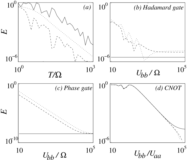
Figure 2: Log-log plot of the gate error, $E=1-{\cal F}$, for different local and nonlocal gates. (a) Realization based on Hamiltonians (1)-(2), with fixed parameters and varying time. We plot the error for the Hadamard (solid), phase (dashed) and CNOT gates (dotted). (b-d) Errors for our proposal with atomic ensembles. We fix the the total time all parameters except the interaction constant $U_{bb}$. In (b-c) we plot realizations for $n=1$ (solid) and $n=3,5$ (dashed) atoms per lattice site. In (d) we plot simulations with a difference of atoms of $|n-m|=0,1,2$ between both wells (solid, dash and dotted lines). The vaues of the parameters are given in the text.

In Fig. 2(a) we illustrate the performance of our method, as well as its sensitivity against non–adiabatic processes. As a figure of merit we have chosen the gate fidelity Nielsen ${\cal F}=|\mathrm{Tr}\{U_{ideal}^{\dagger}U_{real}\}|^{2}/d^{2}$, where $d$ is the dimensionality of the space ($2$ for local gates, $4$ for two-qubit gates), $U_{ideal}$ is the gate that we wish to produce and $U_{real}$ is the actual operation performed. As expected, for fixed parameters $\{\Delta_{m}/\Omega_{m}=\tilde{\Delta}_{m}/\tilde{\Omega}_{m}=1/10,\varphi_{m}=\pi/4\}$, the adiabatic theorem applies when the processes are performed with a sufficiently slow speed. Typically a time $T\sim 300/\Omega_{m},300/\tilde{\Omega}_{m}$ is required for the desired fidelity ${\cal F}=1-10^{-4}$.

Let us now consider a set of bosonic atoms confined in a periodic optical lattice at sufficiently low temperature (such that only the first Bloch band is occupied). The atoms have two relevant internal (ground) levels, $|a\rangle$ and $|b\rangle$, in which the qubit is stored. This set-up has been considered in Ref. QC-mott where it has been shown how single quantum gates can be realized using lasers and two–qubit gates by displacing the atoms that are in a particular internal state to the next neighbor location. The basic ingredients of such a proposal have been recently realized experimentally Bloch2 . However, in this and all other schemes so far williams it is assumed that there is a single atom per lattice site since otherwise even the concept of qubit is no longer valid. In present experiments, in which the optical lattice is loaded with a Bose-Einstein condensate Jaksch1 ; Bloch1 , this is not the case (since zero temperature is required and the number of atoms must be identical to the number of lattice sites). We show now a novel implementation in which, with the help of the methods presented above, one overcomes this problem.

For us a qubit will be formed by an aggregate of atoms at some lattice site. The number of atoms forming each qubit is completely unknown. The only requirement is that there is at least one atom per site superfluid . We will denote by $n_{k}$ the number of atoms in the $k$–th well and identify the states of the corresponding qubit as

$$|{0}\rangle_{k}=\frac{a_{k}^{\dagger n_{k}}}{\sqrt{n!}}|{{\text{v}ac}}\rangle,\quad|{1}\rangle_{k}=b^{\dagger}_{k}\frac{a_{k}^{\dagger(n_{k}-1)}}{\sqrt{(n_{k}-1)!}}|{{\text{v}ac}}\rangle,$$ (9)

where $a_{k}^{\dagger}$ ($b_{k}^{\dagger}$) are the creation operators for one atom in levels $|a\rangle$ and $|b\rangle$, respectively. The quantum gates will be realized using lasers, switching the tunneling between neighboring sites, and using the atom–atom interaction.

In the absence of any external field, the Hamiltonian describing our system is

$$H=-J^{(b)}_{k}\sum_{k}(b^{\dagger}_{k+1}b_{k}+b^{\dagger}_{k}b_{k+1})+\frac{U_{bb}}{2}\sum_{k}b^{\dagger}_{k}b^{\dagger}_{k}b_{k}b_{k}.$$ (10)

Here, $U_{bb}$ and $J^{(b)}_{k}$ describe the interactions between and the tunneling of atoms in state $|b\rangle$. We will assume that $J^{(b)}_{k}$ can be set to zero and increased by adjusting the intensities of the lasers which create the optical lattice. We have assumed that the atoms in state $|a\rangle$ do not interact at all and do not hop, something which may be achieved by tuning the scattering lengths and the optical lattice. Both restrictions will be relaxed later on. The Hamiltonian (10) possesses a very important property when all $J^{(b)}_{k}=0$, namely it has no effect on the computational basis (i.e. $H|\Psi\rangle=0$ for all states $|\Psi\rangle$ in the Hilbert space generated by the qubits). Otherwise, it would produce a non–trivial evolution that would spoil the computation.

We show now how a single qubit gate on qubit $k$ can be realized using lasers. First, during the whole operation we set $J^{(b)}_{k}=0$ in order to avoid hopping. The laser interaction is described by the Hamiltonian

$$H_{las}^{(k)}=\frac{\Delta_{k}}{2}(a^{\dagger}_{k}a_{k}-b^{\dagger}_{k}b_{k})+\frac{\Omega_{k}}{2}(e^{i\varphi}a^{\dagger}_{k}b_{k}+e^{-i\varphi}b^{\dagger}_{k}a_{k}).$$ (11)

For $U_{bb}\gg|\Delta_{k}|,|\Omega_{k}|$, we can project the total Hamiltonian acting on site $k$ by an effective Hamiltonian acting on the qubit which resembles (1), with $\Delta=\Delta_{k}$ and $\Omega=\Omega_{k}\sqrt{n_{k}-1}$. Thus, using the methods exposed above we can achieve the Hadamard and phase gates with a high precision, even though the coupling between the bosonic ensemble and light depends on the number of atoms.

For the realization of the two-qubit Hamiltonian (2) we need to combine several elements. First of all we need the Raman coupling of Eq. (11) to operate on the second well. Second, we need to tilt the lattice using a magnetic field Bloch1 which couples to states $|{a}\rangle$ and $|{b}\rangle$ differently, $H_{tilt}=\sum_{k}kg(a^{\dagger}_{k}a_{k}-b^{\dagger}_{k}b_{k})$. And finally we must allow virtual hopping of atoms of the type $|{b}\rangle$ ($J^{(b)}\ll|U_{bb}-g|$). After adiabatic elimination we find that the effective Hamiltonian depends on the number of particles in the second site, $n_{2}$,

$$H_{2}^{eff}=\frac{J_{b}^{2}}{g-U_{bb}}|{11}\rangle\langle{11}|+\sqrt{n_{2}-1}\tilde{\Omega}\;\hbox{$\mathrm{I}$\kern-6.00006pt$\mathrm{1}$}\otimes\sigma_{x}.$$ (12)

The identification with Eq. (2) is evident, and once more the use of adiabatic passage will produce gates which are independent of the number of particles.

We have studied the different sources of error which may affect our proposal: (i) $U_{bb}$ is finite and (ii) atoms in state $|{a}\rangle$ may hop and interact. These last phenomena are described by additional contributions to Eq. (10) which are of the form $J^{(a)}_{k}(a^{\dagger}_{k}a_{k+1}+a^{\dagger}_{k+1}a_{k})$, $U_{aa}a^{\dagger}_{k}a^{\dagger}_{k}a_{k}a_{k}$, and $U_{ab}a^{\dagger}_{k}b^{\dagger}_{k}a_{k}b_{k}$. The consequences of both imperfections are: (i) more than one atom per well can be excited, (ii) the occupation numbers may change due to hopping of atoms and (iii) by means of virtual transitions the effective Hamiltonian differs from (1) and (2). The effects (i)-(ii) are eliminated if $(\Omega/U_{bb})^{2}\ll 1$ and $(J^{(a)}_{k}/U_{bb})^{2}\ll 1$. Once these conditions are met, we may analyze the remaining errors with a perturbative study of the Hamiltonians (11) and (10) plus the terms ($J^{(a)},U_{ab},U_{aa}$) that we did not consider before. In Eq. (11), the virtual excitation of two atoms increments the parameter $\Delta$ by an unknown amount, $\Delta_{eff}\sim\Delta+2\Omega^{2}n_{k}/(\Delta+U_{ab}-U_{bb})$. If $U_{ab}\ll U_{bb}$ and $\Omega^{2}n_{k}T/U_{bb}\ll 1$, this shift may be neglected. In the two-qubit gates the energy shifts are instead due to virtual hopping of all types of atoms. They are of the order of $\max(J^{(b)},J^{(a)})^{2}/g^{2}\sim J^{2}/U_{bb}$, and for $J^{2}T/U_{bb}\ll 1$ they also may be neglected.

To quantitatively determine the influence of these errors we have simulated the evolution of two atomic ensembles with an effective Hamiltonian which results of applying second order perturbation theory to Eq. (10), and which takes into account all important processes. The results are shown in Figs. 2(c-d). For the two-qubit gate we have assumed $U_{aa}=U_{ab}$, $J^{(a)}=J^{(b)}=J$, $J_{m}=0.05U_{ab}$, $\Omega_{m}=J_{m}^{2}/10$, $g=U_{bb}+U_{ab}/2$ and operation time, $T=200/\Omega_{m}$, while changing the ratio $U_{bb}/U_{ab}$ and the populations of the wells. For the local gates we have assumed $\Delta_{m}=1$, $\Omega_{m}=U_{bb}/10$ and different occupation numbers $n_{k}$, and we have also changed $U_{bb}/\Omega_{m}$.

We extract several conclusions. First, the stronger the interaction between atoms in state $|{b}\rangle$, the smaller the energy shifts. Typically, a ratio $U_{bb}=10^{4}U_{ab}$ is required to make ${\cal F}=1-10^{-4}$. Second, the larger the number of atoms per well, the poorer the fidelity of the local gates [Figs. 2(b-c)]. And finally, the fidelity of the two-qubit gate presents a small dependence on the population imbalance between wells.

In this work we have shown that it is possible to perform quantum computation even when the constants in the governing Hamiltonians are unknown. We have developed a scheme based on performing adiabatic passage with one-qubit (1) and two-qubit (2) Hamiltonians. With selected paths and appropriate timing, it is possible to perform a universal set of gates (Hadamard gate, phase gate and a CNOT). These procedures cannot only be used for quantum computing but also for quantum simulation Guifre . Finally, based on the preceding ideas, we have proposed a scheme for quantum computing with cold atoms in a tunable optical lattice. Our scheme works even when the number of atoms per lattice site is uncertain. Note that, these ideas also apply to some other setups like the microtraps recently realized in Ref. Ertmer .

We thank D. Liebfried and P. Zoller for discussions and the EU project EQUIP (contract IST-1999-11053).

References

- (1) Note that, in principle, one could measure the dependence of these parameters (function ). However in many realistic implementations this is not possible, since the measurements are destructive (lead to heating or the atoms escape the trap), and in different realizations the dependence is different.
- (2) A. M. Steane, arXiv:quant-ph/0207119; P. W. Shor, in Proc. 35th Annual Symposium on Fundamentals of Computer Science (IEEE Press, Los Alamitos, 1996), p. 56, arXiv:quant-ph/9605011; E. Knill, R. Laflamme, and W. H. Zurek, Science 279, 342 (1998); D. Aharonov and M. Ben-Or, SIAM Jour. Comput. (submitted) arXive:quant-ph/9906129.
- (3) J. I. Cirac, and P. Zoller Phys. Rev. Lett. 74, 4091 (1995); C. Monroe et al. Phys. Rev. Lett. 75, 4714 (1995).
- (4) M. Greiner et al., Nature 415, 39 (2002).
- (5) See, for example, M. A. Nielsen and I. L. Chuang, Quantum Computation and Quantum Information (Cambridge Univ. Press, Cambridge, 2002).
- (6) D. Jaksch et al., Phys. Rev. Lett. 81, 3108 (1998).
- (7) D. Jaksch et al., Phys. Rev. Lett. 82, 1975 (1999).
- (8) P. Zanardi and M. Rasetti, Phys. Lett. A 264, 94 (1999); J. Pachos, P. Zanardi, M. Rasetti, Phys. Rev. A 61, 010305(R)a (2000).
- (9) J. A. Jones et al, Nature 403, 869 (1999); G. Falci, et al., Nature 407, 355 (2000)
- (10) L.-M. Duan, J. I. Cirac, and P. Zoller, Science 292, 1695 (2001); A. Recati et al. , arXiv:quant-ph/0204030.
- (11) L. Viola, and S. Lloyd, Phys. Rev. A 58, 2733 (1998); L.-M. Duan, and G. Guo, arXiv:quant-ph/9807072
- (12) I. Bloch (private communication).
- (13) E. Charron et al., Phys. Rev. Lett. 88, 077901 (2002); K. Eckert et al., arXiv:quant-ph/0206096.
- (14) The current scheme would even work with a superfluid phase which is abruptly loaded in a deep optical lattice.
- (15) E. Jané et al., arXiv:quant-ph/0207011.
- (16) R. Dumke et al., Phys. Rev. Lett. 89, 097903 (2002).