Decoherence of molecular wave packets in an anharmonic potential

Abstract

The time evolution of anharmonic molecular wave packets is investigated under the influence of the environment consisting of harmonic oscillators. These oscillators represent photon or phonon modes and assumed to be in thermal equilibrium. Our model explicitly incorporates the fact that in the case of a nonequidistant spectrum the rates of the environment induced transitions are different for each transition. The nonunitary time evolution is visualized by the aid of the Wigner function related to the vibrational state of the molecule. The time scale of decoherence is much shorter than that of dissipation, and gives rise to states which are mixtures of localized states along the phase space orbit of the corresponding classical particle. This behavior is to a large extent independent of the coupling strength, the temperature of the environment and also of the initial state.

I introduction

The correspondence between classical and quantum dynamics of anharmonic systems has gained significant attention in the past few years Parker and Stroud (1986); Averbukh and Perelman (1989); Vetchinkin and Eryomin (1994); Aronstein and C. R. Stroud (2000). A short laser pulse impinging on an atom or a molecule excites a superposition of several stationary states, and the resulting wave packet follows the orbit of the corresponding classical particle in the initial stage of the time evolution.

However, the nonequidistant nature of the involved energy spectra causes peculiar quantum effects, broadening of the initially well localized wave packets, revivals and partial revivals Averbukh and Perelman (1989); Parker and Stroud (1986); Vetchinkin and Eryomin (1994); Aronstein and C. R. Stroud (2000); Leichtle et al. (1996); Domokos et al. (2000). Partial revivals are in close connection with the formation of Schrödinger-cat states, which, in this context, are coherent superpositions of two spatially separated, well localized wave packets Janszky et al. (1994). Phase space description of vibrational Schrödinger-cat state formation using animated Wigner functions can be found in Földi et al. (2002). However, these highly nonclassical states are expected to be particularly sensitive to decoherence Giulini et al. (1996). The aim of this paper is to analyze the process of decoherence for the spontaneously formed Schrödinger-cat states in the anharmonic potential.

We consider the decoherence model which relies on the interaction of the quantum system (S) with its environment (E) that has many degrees of freedom. The dynamics of the environment together with the quantum system under investigation is unitary, i.e., the density operator $\rho_{SE}$ of the coupled $S+E$ system always represents a pure state. Starting from an initially uncorrelated density operator, the interaction builds up S–E entanglement and the reduced density operator

$$\rho_{S}=\mathrm{Tr}_{E}\left(\rho_{SE}\right),$$ (1)

where $\mathrm{Tr}_{E}$ means a trace over the environmental degrees of freedom, turns into a mixture. Assuming negligibly short relaxation times in the environment, one obtains a Markovian master equation which is a useful tool for the dynamical investigation of the environment induced decoherence. It allows for the determination of pointer states Zurek (1981), that is, states that are favored by decoherence Zurek et al. (1993); Földi et al. (2001), and also for the calculation of the characteristic time of decoherence for different initial states Földi et al. (2001); Benedict and Czirják (1999).

In the following we introduce a master equation that takes into account the fact that in a general anharmonic system the relaxation rate of each energy eigenstate is different. This master equation is applied to the case of wave packet motion in the Morse potential that is often used to describe a vibrating diatomic molecule. Considering the phase-space description of decoherence, we show how the phase portrait of the system reflects the damping of revivals in the expectation values of the position and momentum operators due to the effect of the environment. We also calculate and plot the time evolution of the Wigner function corresponding to the reduced density operator of the Morse system. The Wigner function picture visualizes the fact that although our master equation reduces to the amplitude damping equation Walls and Milburn (1985); Savage and Walls (1985); Phoenix (1990); Bužek et al. (1992) in the harmonic limit, the anharmonic effects lead to a decoherence scheme which is similar to the phase relaxation Walls and Milburn (1985) of the harmonic oscillator (HO). It is found that the reduced density operator that arises due to the decoherence can be identified with a mixture of states that are well-localized in the phase space and equally distributed along the orbit of the corresponding classical particle. We illustrate the generality of this decoherence scheme by presenting the time evolution of an energy eigenstate as well. We also calculate the decoherence time for various initial wave packets. We show that decoherence is faster for wave packets that correspond to a classical particle with a phase space orbit of larger diameter.

II Description of the model

The total Hamiltonian of an anharmonic system and its environment has the form

$$H_{S+E}=H_{S}+H_{E}+V.$$ (2)

The self-Hamiltonian of the system is written as:

$$H_{S}=\sum_{n}E_{n}|\phi_{n}\rangle\langle\phi_{n}|,$$ (3)

where the spectrum $\{E_{n}\}$ is assumed to be nondegenerate and discrete, but not necessarily equidistant. $E_{0}$ denotes the ground state energy of the system, and $E_{m}>E_{n}$ whenever $m>n$. The environment is represented by a set of harmonic oscillators

$$H_{E}=\sum_{k}\hbar\omega_{k}(a^{\dagger}_{k}a_{k}+1/2).$$ (4)

We assume the following interaction Hamiltonian

$$V=\hbar\mathcal{X}^{\dagger}\sum_{k}g_{k}a_{k}+\hbar\mathcal{X}\sum_{k}g_{k}a^{\dagger}_{k},$$ (5)

where $\mathcal{X}$ is an appropriate system operator that transforms each eigenstate of $H_{S}$ into a superposition of different eigenstates corresponding to lower energy values. This is the application of the rotating wave approximation (RWA) to an anharmonic, multilevel system. The operator $\mathcal{X}^{\dagger}$ is the Hermitian conjugate of $\mathcal{X}$, and for the sake of simplicity the coupling constants $g_{k}$ were taken to be real. In the case of a vibrating diatomic molecule $H_{E}$ describes the modes of the free electromagnetic field, while the terms $\mathcal{X}$ and $\mathcal{X}^{\dagger}$ in the interaction Hamiltonian are related to the molecular dipole moment operator.

We assume that the environment is in thermal equilibrium at a given temperature $T$, and the environmental oscillators have continuous distribution with frequency dependent density of states, $D(\omega)$. Starting from the von Neumann equation for the total density operator, standard techniques Nakajima (1958); Zwanzig (1960); Haake (1973); Walls and Milburn (1994) lead to the following Markovian master equation in the Schrödinger picture

$$\frac{d}{dt}\rho_{S} = -{\frac{i}{\hbar}}\left[H_{S},\rho_{S}\right]-\big{(}\mathcal{X}^{\dagger}\mathcal{X}_{e}\rho_{S}+\mathcal{X}\mathcal{X}_{a}^{\dagger}\rho_{S}$$ (6)

$$- \mathcal{X}_{a}^{\dagger}\rho_{S}\mathcal{X}-\mathcal{X}_{e}\rho_{S}\mathcal{X}^{\dagger}+\mathrm{h.c.}\big{)}.$$

The matrix elements of the operators appearing in the nonunitary terms are given by

$$\langle\phi_{m}|\mathcal{X}_{a}|\phi_{n}\rangle = \pi\langle\phi_{m}|\mathcal{X}|\phi_{n}\rangle\ D(\omega_{nm})g^{2}(\omega_{nm})\overline{n}(\omega_{nm}),$$

$$\langle\phi_{m}|\mathcal{X}_{e}|\phi_{n}\rangle = \pi\langle\phi_{m}|\mathcal{X}|\phi_{n}\rangle\ D(\omega_{nm})g^{2}(\omega_{nm})$$ (7)

$$\times \left(\overline{n}(\omega_{nm})+1\right),$$

where $\omega_{nm}=|E_{m}-E_{n}|/\hbar$, $\overline{n}(\omega)=({\exp{\frac{\hbar\omega}{kT}}-1})^{-1}$ denotes the average number of quanta in the corresponding mode of the environment, and the subscripts $e$ and $a$ refer to emission and absorption, respectively.

As we can see, the matrix elements (7) of the operators that induce the transitions depend on the Bohr frequency of the involved transition, which is a genuine anharmonic feature. In the special case of the HO, when $H_{S}$ has equidistant spectrum, and $\mathcal{X}$ is identified with the usual annihilation operator $a$, both $\mathcal{X}_{a}$ and $\mathcal{X}_{e}$ are proportional to $\mathcal{X}\equiv a$, and Eq. (6) reduces to the amplitude damping master equation Walls and Milburn (1985); Savage and Walls (1985); Phoenix (1990); Bužek et al. (1992) at a finite temperature.

In certain cases one can further simplify Eq. (6). When the environment induced relaxation rates are much lower than the relevant Bohr frequencies, the system Hamiltonian induces oscillations that are very fast even on the time scale of decoherence and vanish on the average. Ignoring these fast oscillations we arrive at the interaction picture master equation

$$\frac{d}{dt}\langle\phi_{i}|\rho_{S}|\phi_{j}\rangle=\delta_{i,j}\sum_{k\neq i}\gamma_{ik}\langle\phi_{k}|\rho_{S}|\phi_{k}\rangle-\Gamma_{ji}^{c}\langle\phi_{i}|\rho_{S}|\phi_{j}\rangle,$$ (8)

that has already been obtained in Refs. Lax (1966); Agarwal (1973) in order to treat the spontaneous emission of a multilevel atom. In Eq. (8), $\gamma_{ik}$ denotes a relaxation rate, that is the probability of the $|\phi_{k}\rangle\rightarrow|\phi_{i}\rangle$ transition per unit time, while $\Gamma_{ji}^{c}=1/2\sum_{k}(\gamma_{ik}+\gamma_{jk})$, where

$$\gamma_{ik}=\left\{\begin{array}[]{lr}2\ \langle\phi_{i}|\mathcal{X}_{e}|\phi_{k}\rangle\langle\phi_{i}|\mathcal{X}|\phi_{k}\rangle&{\textnormal{if}}\ i<k,\\ 0&{\textnormal{if}}\ i=k,\\ 2\ \langle\phi_{i}|\mathcal{X}_{a}|\phi_{k}\rangle\langle\phi_{i}|\mathcal{X}|\phi_{k}\rangle&{\textnormal{if}}\ i>k.\end{array}\right.$$ (9)

However, due to the elimination of the fast oscillations related to $H_{S}$, Eq. (8) is not suitable for investigating the wave packet motion and decoherence simultaneously, therefore we propose to use Eq. (6). On the other hand we note that Eq. (8) radically reduces the computational costs of calculating the time evolution for long times, which might be necessary when the system-environment coupling is very weak.

Supposing that our knowledge is limited to the populations $P_{n}=\langle\phi_{n}|\rho_{s}|\phi_{n}\rangle$, both Eq. (6) and Eq. (8) leads to the Pauli type equation

$$\frac{d}{dt}P_{n}=\sum_{k}\left(\gamma_{nk}P_{k}-\gamma_{kn}P_{n}\right).$$ (10)

Requiring the condition of detailed balance Reif (1965) in Eq. (10) leads to the steady-state thermal distribution at the temperature of the environment.

When a diatomic molecule is considered in the environment of the free electromagnetic field, the operators $\mathcal{X}$ and $\mathcal{X}^{\dagger}$ in Eq. (5) gain a clear interpretation: in the eigenbasis of $H_{S}$ they are the upper and lower triangular parts of the molecular dipole moment operator, $\hat{\mu}$. We will assume that $\hat{\mu}$ is linear Yuan and Liu (1998), that is, proportional to the displacement $X$ of the center of mass of the diatomic system from the equilibrium position. In this case $g^{2}(\omega)D(\omega)\propto\omega^{3}$, that is,

$$\langle\phi_{m}|\mathcal{X}_{a}|\phi_{n}\rangle = \lambda\ \langle\phi_{m}|X|\phi_{n}\rangle\ {\omega_{nm}}^{3}\ \overline{n}(\omega_{nm}),$$

$$\langle\phi_{m}|\mathcal{X}_{e}|\phi_{n}\rangle = \lambda\ \langle\phi_{m}|X|\phi_{n}\rangle\ {\omega_{nm}}^{3}\left(\overline{n}(\omega_{nm})+1\right),$$ (11)

where matrix elements of $X$ can be calculated using the algebraic method summarized in Benedict and Molnár (1999), and $\lambda=\pi g^{2}(\omega)D(\omega)/\omega^{3}$ is an overall, frequency independent coupling constant.

However, in order to get insight into the interplay between wave packet motion and decoherence, it is worth considering a stronger molecule-environment interaction than the electromagnetic field modes can provide. Keeping the structure of Eqs. (11), this can be done by increasing the value of $\lambda$. Here we present calculations with two different coupling constants, $\lambda_{1}$ and $\lambda_{2}$ which are chosen so that at zero temperature $\omega_{01}/\gamma_{01}\approx 10^{5}$ and $4\times 10^{3}$ for $\lambda=\lambda_{1}$ and $\lambda_{2}$, respectively. This model allows for the numerical integration of the master equation (6) (that provides more details of the dynamics than Eq. (8)) in a time interval that is long enough to identify the effects of decoherence. These effects can be summarized in a decoherence scheme (see Sec. V) that has a clear physical interpretation, and which is valid also in the weak molecule-environment interaction, when (8) is more efficient to calculate the time evolution.

In the following we shall apply our master equation (6) to the case of the Morse Hamiltonian Huber and Herzberg (1979) that is often used to describe a vibrating diatomic molecule. This Hamiltonian has the dimensionless form

$$H_{S}=P^{2}+(s+1/2)^{2}[\exp(-2X)-2\exp(-X)],$$ (12)

where the shape parameter $s$ is related to the dissociation energy $D_{\mathrm{diss}}$, the reduced mass of the molecule $m$, and the range parameter of the potential $\alpha$ via $s=\frac{\sqrt{2mD_{\mathrm{diss}}}}{\hbar\alpha}-1/2.$ The dimensionless displacement and momentum operators obey the canonical commutation relation $[X,P]=i$.

The Hamiltonian (12) sustains $[s]+1$ normalizable eigenstates (bound states), corresponding to the eigenvalues $E_{m}(s)=-(s-m)^{2},$ $m=0,1,\ldots[s]$, where $[s]$ denotes the largest integer that is smaller than $s$. The continuum above $E_{m=[s]}$ corresponds to the dissociated molecule with positive energies. For the sake of definiteness we have chosen the NO molecule as our model, where $s=54.54$.

The initial wave packets of our analysis will be Morse coherent states Benedict and Molnár (1999), $|x_{0},p_{0}\rangle$, which are localized on the phase space around the point $(x_{0},p_{0})$. The Wigner function of a representative Morse coherent state is shown in Fig. 3 a). These states can be prepared by an appropriate electromagnetic pulse that drives the vibrational state of the molecule starting from the ground state into an approximate coherent state. An example can be found in Molnár et al. (2001), where the effect of an external sinusoidal field is considered.

Let us note that the construction given in Molnár et al. (2002) would allow us to use arbitrary initial states, but for our current purpose it suffices to consider states $|x_{0},p_{0}\rangle$ with negligible dissociation probability, i.e., coherent states that practically can be expanded in terms of the bound states $|\phi_{n}\rangle$, $n=0,1,\ldots[s]$.

III Time evolution of the expectation values

Starting from $|\psi(t=0)\rangle=|x_{0},p_{0}=0\rangle$ as initial states, the qualitative behavior of the expectation value $\langle X\rangle(t)=\langle\psi(t)|X|\psi(t)\rangle$ draws the limit of small oscillations. In the absence of environmental coupling (i.e., $\lambda=0$), for $x_{0}\leq 0.05$, $\langle X\rangle(t)$ (as well as $\langle P\rangle(t)$) exhibits sinusoidal oscillations.

\psfrag{plabel}[tl][tl]{$\langle P\rangle$}\psfrag{xlabel}{$\langle X\rangle$}\psfrag{tlabel}{$t/t_{0}$}\includegraphics*[bb=80 50 670 470,width=241.84842pt]{foldifig1.eps}

Figure 1: Phase portrait corresponding to the time evolution of the initial state $|\psi(t=0)\rangle=|x_{0},0\rangle$, with $x_{0}=0.5$. The parameters are $\lambda=\lambda_{1}$, $T=5\ \hbar\omega_{01}/k$, and $t_{0}$ is the period of the small oscillations in the potential. The initial point $\langle X\rangle=0.5$, $\langle P\rangle=0$ together with the starting direction is also indicated.

For larger initial displacements from the equilibrium position, the anharmonic effects become apparent: the amplitude of the oscillations decreases almost to zero, then faster oscillations with small amplitude appear but later we re-obtain almost exactly $\langle X\rangle(0)$ (and $\langle P\rangle(0)$ as well), and the whole process starts again Földi et al. (2002). Without the influence of the environment the main attributes of $\langle X\rangle(t)$ and $\langle P\rangle(t)$ can be explained by referring to the various Bohr frequencies that determine their time dependence: dephasing of these frequencies leads to the collapse of the expectation value, and we observe revival when they rephase again.

For the initial state of $|\psi(t=0)\rangle=|x_{0},0\rangle$, with $x_{0}=0.5$, the original phase of the eigenstates is restored Parker and Stroud (1986); Averbukh and Perelman (1989) around the full revival time $t_{rev}=110\ t_{0}$, where $t_{0}$ is the period of the small oscillations in the potential. At $t/t_{0}=55$ and $t/t_{0}=27.5$ half and quarter revivals Parker and Stroud (1986); Averbukh and Perelman (1989) can be observed. Fig. 1 shows the damping of the revivals both in $\langle X\rangle(t)$ and $\langle P\rangle(t)$ when interaction with the environment is turned on. Note that the phase portrait of the corresponding classical particle would be a helix with monotonically decreasing diameter, revivals are of quantum nature. However, Fig. 1 does not provide a complete description of the time evolution in the phase space, this can be given by using Wigner functions, see Sec. V.

IV Decoherence times

Our master equation (6) describes decoherence as well as dissipation. However, the time scale of these processes is generally very different, and one can distinguish the stages of the time evolution that are dominated either by decoherence or dissipation Földi et al. (2001).

\psfrag{elabel}[tl][tl][0.8]{$S(t)$}\psfrag{trlabel}[bl][bl][0.8]{$\mathrm{Tr}\left[\rho_{S}^{2}(t)\right]$}\psfrag{eaxis}{$S$}\psfrag{traxis}[br][bl]{$\mathrm{Tr}\rho_{S}^{2}$}\psfrag{taxis}{$t/t_{0}$}\includegraphics*[bb=65 45 775 515,width=241.84842pt]{foldifig2.eps}

Figure 2: The entropy and the purity of the reduced density matrix of the Morse system as a function of time, calculated using Eq. (6). The coupling parameter (see Sec. II) is $\lambda=\lambda_{1}$ and $T=10\ \hbar\omega_{01}/k$. The initial state was $|\psi(t=0)\rangle=|x_{0},0\rangle$, with $x_{0}=2.0$.

In Fig. 2 an example is depicted showing how the method of time scale separation works. We have calculated the entropy

$$S=-\mathrm{Tr}\left[\rho_{S}\ln(\rho_{S})\right],$$ (13)

as well as the quantity $\mathrm{Tr}[\rho_{S}^{2}]$, which measures the purity of the reduced density operator. Note that the $\mathrm{Tr}$ operation without subscript refers to the trace in the system’s Hilbert space. Decoherence time $t_{d}$ is defined as the time instant that divides the time axis into two parts where the character of the physical process is clearly different. Initially both $S(t)$ and $\mathrm{Tr}[\rho_{S}^{2}(t)]$ change rapidly but having passed $t_{d}$ (emphasized by a vertical line in Fig. 2), the moduli of their derivative significantly decrease. After $t_{d}$ the entropy and the purity change on the time scale which is characteristic of the dissipation of the system’s energy during the whole process Benedict and Czirják (1999); Földi et al. (2001). In other words, decoherence dominated time evolution turns into dissipation dominated dynamics around $t_{d}$. In the next section we shall determine the density operators into which the process of decoherence drives the system. In connection with these results we have verified that the states around the decoherence time do not change appreciably in a time interval that covers the possible errors in determining $t_{d}$.

An interesting question is the dependence of the decoherence time on the initial state of the time evolution. We calculated $t_{d}$ as a function of the initial displacement for the case of displaced ground states (that is, coherent states with zero momentum, $|x_{0},0\rangle$) as initial states. It was found that for all values of $\lambda$ and $T$, the decoherence time is longer for smaller initial displacements. Additionally, for fixed $\lambda$ and $T$ the function $t_{d}(x_{0})$ can be well approximated by an exponential curve $t_{d}(x_{0})=t_{d}(0)\exp(-\kappa x_{0})$. E. g., for $\lambda=\lambda_{1}$, $T=10\ \hbar\omega_{01}/k$ and $0<x_{0}\leq 2$ the parameters take the values $t_{d}(0)=93\ t_{0}$ and $\kappa=0.97$.

It is known Averbukh and Perelman (1989) that quarter revivals in an anharmonic potential lead to the formation of Schrödinger-cat states, i.e., states that are superpositions of two distinct states localized in space Averbukh and Perelman (1989) as well as in momentum Földi et al. (2002); Kasperkovitz and Peev (1995). On the other hand, smaller initial displacements correspond to classical phase space orbits with smaller diameter. Consequently the quantum interference related to nonclassical states that are formed during the course of time cover a smaller area in the phase-space in this case. This means that our result is a manifestation of the general feature of decoherence that increasing the “parameter of nonclassicality”, which is the diameter of the corresponding classical orbit in our case, causes faster decoherence Giulini et al. (1996). A similar result was found in Földi et al. (2001) for the case of decoherence in a system of two-level atoms Benedict and Czirják (1999); Braun et al. (2000).

V Wigner function description of the decoherence

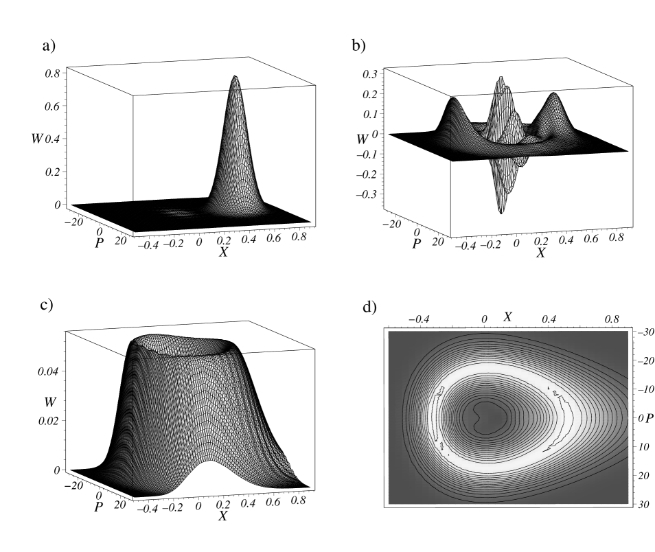
Figure 3: Time evolution of the Wigner function corresponding to the initial state $|\psi(t=0)\rangle=|x_{0},0\rangle$, with $x_{0}=0.5$. The coupling parameter is (see Sec. II) $\lambda=\lambda_{2}$ and $T=0.3\ \hbar\omega_{01}/k$. The plots a) and b) correspond to time instants $t/t_{0}=0\ \text{and}\ 27.5$, while both c) and the contour plot d) are snapshots taken at $t/t_{0}=137.5$.

In order to visualize the time evolution of the reduced density matrix of the Morse system we have chosen the Wigner function picture, which represents $\rho_{S}$ as a function over the classical phase space

$$W(x,p,t)={\frac{1}{2\pi}}\int_{-\infty}^{\infty}\langle x-u/2|\rho_{S}(t)|x+u/2\rangle e^{iup}du.$$ (14)

This description allows us to investigate the correspondence between classical and quantum dynamics.

First we consider the ideal case without environment. Then, in the initial stage of the time evolution, the positive hill corresponding to the wave packet $|x_{0},p_{0}\rangle$ follows the orbit of the classical particle that has started from $(x_{0},p_{0})$ at $t=0$. However, due to the uncertainty relation, the Wigner function as a quasiprobability distribution has a finite width, and this fact combined with the form of the Morse potential implies the stretching of the Wigner function along the classical orbit in the course of time. (See Ref. Kasperkovitz and Peev (1995) for similar results with the Husimi $Q$ function.) After a certain time the increasingly broadened wave packet becomes able to interfere with itself, and around the quarter revival time one can observe two positive hills chasing each other at the opposite sides of the classical orbit. The strong oscillations of $W$ between the hills represent the quantum correlation of the constituents of this molecular Schrödinger-cat state Janszky et al. (1994). Later on the initial Wigner function is restored almost exactly and Schrödinger-cat state formation starts again. Detailed Wigner function description of these processes that are related to the free time evolution can be found in Földi et al. (2002).

In the case when environmental effects are present, we found that decoherence follows a general scheme. A representative series of Wigner functions is shown in Fig. 3. The snapshots correspond to the initial state and time instants when the first and third Schrödinger-cat state formation would occur in the absence of the environment. Consequently, the Wigner function in Fig. 3 b) corresponds almost to a Schrödinger-cat state, but this state is already a mixture. However, there are still negative parts of the function in between the positive hills centered at $x_{1}=0.51,\ p_{1}=0$ and $x_{2}=-0.34,\ p_{2}=0$. The “ridge” that connects these hills along the classical orbit is absent in a pure Schrödinger-cat state. Later on this ridge becomes more and more pronounced and at the decoherence time we arrive at the positive Wigner function of Fig. 3 c) and d). According to the contour plot Fig. 3 d), the highest values of this function trace out the phase space orbit of the corresponding classical particle. That is, $\rho_{S}^{dec}$, the reduced density matrix that arises as a result of decoherence, can be interpreted as a mixture of localized states that are equally distributed along the orbit of the corresponding classical phase space orbit.

Figure 4: Time evolution of the Wigner function corresponding to the fifth bound state as initial state. The coupling parameter (see Sec. II) is $\lambda=\lambda_{1}$ and $T=10\ \hbar\omega_{01}/k$. The plots a), b), c) and d) correspond to time instants $t/t_{0}=0,\ 27.5,\ 330$ and $1000$, respectively.

It is worth comparing this result with the case of the HO, when the master equation (6) reduces to the amplitude damping equation Walls and Milburn (1985); Savage and Walls (1985); Phoenix (1990); Bužek et al. (1992), see Sec. II. It is known that harmonic oscillator coherent states are robust against the decoherence described by the amplitude damping master equation (as well as against the Caldeira-Leggett Caldeira and Leggett (1983) master equation Zurek et al. (1993)), the initial superposition of coherent states turns into the statistical mixture of essentially the same states. This is a consequence of the facts that these states are eigenstates of the destruction operator $a$, and the operators in the nonunitary terms of Eq. (6) are proportional to $a$ and $a^{\dagger}$ in the harmonic case. None of these statements can be transferred to the anharmonic system, where the Morse coherent states do not remain localized during the course of time, even without environment. Therefore the scheme of the decoherence is qualitatively different for the harmonic and anharmonic oscillators: Our results in the anharmonic system are similar to the phase relaxation in the harmonic case Walls and Milburn (1985), where the energy of the system remains unchanged, but the phase information is completely destroyed. We note that a similar result was obtained in Ref. Brif et al. (2001), where the rotational degrees of freedom were considered as a reservoir for the harmonic vibration of hot alkaline dimers.

Our decoherence scheme is universal to a large extent. In the investigated domain of the coupling constants $\lambda_{1}\leq\lambda\leq\lambda_{2}$ and temperatures ranging from $T=0$ to $T=15\ \hbar\omega_{01}/k$, it is found to be valid for all initial states, not only for coherent states. Fig. 4 shows an example when the initial state is not a wave packet, it is the fifth bound state, corresponding to $E_{5}$, which is very close to $\langle 0.5,0|H_{S}|0.5,0\rangle$, so direct comparison with Fig. 3 is possible. As we can see, although the two Wigner functions are initially obviously very different, they follow different routes (that takes different times) to the same state: Fig. 3 c) and Fig. 4 c) are practically identical. The final plot in Fig. 4 indicates how the Wigner function represents the long way to thermal equilibrium with the environment: the distribution becomes wider and the hole in the middle disappears.

It is expected that the loss of phase information has observable consequences. According to the Franck-Condon principle, the absorption spectrum of a molecule around the frequency corresponding to an electronic transition between two electronic surfaces depends on the vibrational state. The time dependence of the spectrum should exhibit the differences between the pure state of an oscillating wave packet and the state $\rho_{S}^{dec}$ and the thermal state. More sophisticated experimental methods based on the detection of fluorescence Khundkar and Zewail (1990) or fluorescence intensity fluctuations Warmuth et al. (2000), surely have the capacity of observing the dephasing phenomenon considered in this paper.

VI Conclusions

We investigated the decoherence of wave packets in the Morse potential. The decoherence time for various initial states was calculated and it was found that the larger is the diameter of the phase space orbit described by a wave packet, the faster is the decoherence. We obtained a general decoherence scheme, which has a clear physical interpretation: The reduced density operator that is the result of the decoherence is a mixture of states localized along the corresponding classical phase space orbit.

This work was supported by the Hungarian Scientific Research Fund (OTKA) under contracts Nos. T32920, D38267, and by the Hungarian Ministry of Education under contract No. FKFP 099/2001.

References

- Parker and Stroud (1986) J. Parker and C. R. Stroud, Phys. Rev. Lett. 56, 716 (1986).
- Averbukh and Perelman (1989) I. S. Averbukh and N. F. Perelman, Phys. Lett. A139, 449 (1989).
- Vetchinkin and Eryomin (1994) S. I. Vetchinkin and V. V. Eryomin, Chem. Phys. Lett. 222, 394 (1994).
- Aronstein and C. R. Stroud (2000) D. L. Aronstein and J. C. R. Stroud, Phys. Rev. A 62, 022102/1 (2000).
- Leichtle et al. (1996) C. Leichtle, I. S. Averbukh, and W. P. Schleich, Phys. Rev. A 54, 5299 (1996).
- Domokos et al. (2000) P. Domokos, T. Kiss, J. Janszky, A. Zucchetti, Z. Kis, and W. Vogel, Chem. Phys. Lett. 322, 255 (2000).
- Janszky et al. (1994) J. Janszky, A. V. Vinogradov, T. Kobayashi, and Z. Kis, Phys. Rev. A 50, 1777 (1994).
- Földi et al. (2002) P. Földi, A. Czirják, B. Molnár, and M. G. Benedict, Opt. Express 10, 376 (2002).
- Giulini et al. (1996) D. Giulini, E. Joos, C. Kiefer, J. Kupsch, I.-O. Stamatescu, and H. D. Zeh, Decoherence and the Appearance of a Classical World in Quantum Theory (Springer-Verlag, Berlin, Heidelberg, New York, 1996).
- Zurek (1981) W. H. Zurek, Phys. Rev. D 24, 1516 (1981).
- Zurek et al. (1993) W. H. Zurek, S. Habib, and J. P. Paz, Phys. Rev. Lett. 70, 1187 (1993).
- Földi et al. (2001) P. Földi, A. Czirják, and M. G. Benedict, Phys. Rev. A 63, 033807 (2001).
- Benedict and Czirják (1999) M. G. Benedict and A. Czirják, Phys. Rev. A 60, 4034 (1999).
- Walls and Milburn (1985) D. F. Walls and G. J. Milburn, Phys. Rev. A 31, 2403 (1985).
- Savage and Walls (1985) C. M. Savage and D. F. Walls, Phys. Rev. A 32, 2316 (1985).
- Phoenix (1990) S. J. D. Phoenix, Phys. Rev. A 41, 5132 (1990).
- Bužek et al. (1992) V. Bužek, A. Vidiella-Barranco, and P. L. Knight, Phys. Rev. A 45, 6570 (1992).
- Nakajima (1958) S. Nakajima, Prog. Theor. Phys. 20, 948 (1958).
- Zwanzig (1960) R. Zwanzig, J. Chem. Phys. 33, 1338 (1960).
- Haake (1973) F. Haake, Statistical Treatment of Open Systems by Generalized Master Equations (Springer-Verlag, Berlin, 1973), vol. 66 of Springer tracts in modern physics.
- Walls and Milburn (1994) D. F. Walls and G. J. Milburn, Quantum Optics (Springer-Verlag, Berlin, 1994).
- Lax (1966) M. Lax, Phys. Rev. 145, 110 (1966).
- Agarwal (1973) G. S. Agarwal, Master Equation methods in quantum optics (North Holland, 1973), vol. XI of Progress in Optics, pp. 3–73.
- Reif (1965) F. Reif, Fundamentals of Statistical and Thermal Physics (McGraw-Hill, Singapore, 1965).
- Yuan and Liu (1998) Y.-M. Yuan and W.-K. Liu, Phys. Rev. A 57, 1992 (1998).
- Benedict and Molnár (1999) M. G. Benedict and B. Molnár, Phys. Rev. A 60, R1737 (1999).
- Huber and Herzberg (1979) K. P. Huber and G. Herzberg, Molecular spectra and molecular structure IV. Constants of diatomic molecules (van Nostrand Reinhold, 1979).
- Molnár et al. (2001) B. Molnár, M. G. Benedict, and P. Földi, Fortschr. Phys. 49, 1053 (2001).
- Molnár et al. (2002) B. Molnár, P. Földi, M. G. Benedict, and F. Bartha (2002), quant-ph/0202069.
- Kasperkovitz and Peev (1995) P. Kasperkovitz and M. Peev, Phys. Rev. Lett. 75, 990 (1995).
- Braun et al. (2000) D. Braun, P. A. Braun, and F. Haake, Opt. Comm. 179, 411 (2000).
- Caldeira and Leggett (1983) A. O. Caldeira and A. J. Leggett, Physica A 121, 587 (1983).
- Brif et al. (2001) C. Brif, H. Rabitz, S. Wallentowitz, and I. A. Walmsley, Phys. Rev. A 63, 063404 (2001).
- Khundkar and Zewail (1990) L. Khundkar and A. H. Zewail, Annu. Rev. Phys. Chem. 41, 15 (1990), and see also references therein.
- Warmuth et al. (2000) C. Warmuth, A. Tortschanoff, F. Milota, M. Shapiro, Y. Prior, I. S. Averbukh, W. Schleich, W. Jakubetz, and H. F. Kauffmann, J. Chem. Phys. 112, 5060 (2000).