Maximal entanglement versus entropy for mixed quantum states

Abstract

Maximally entangled mixed states are those states that, for a given mixedness, achieve the greatest possible entanglement. For two-qubit systems and for various combinations of entanglement and mixedness measures, the form of the corresponding maximally entangled mixed states is determined primarily analytically. As measures of entanglement, we consider entanglement of formation, relative entropy of entanglement, and negativity; as measures of mixedness, we consider linear and von Neumann entropies. We show that the forms of the maximally entangled mixed states can vary with the combination of (entanglement and mixedness) measures chosen. Moreover, for certain combinations, the forms of the maximally entangled mixed states can change discontinuously at a specific value of the entropy.

I Introduction

Over the past decade, the physical characteristic of the entanglement of quantum-mechanical states, both pure and mixed, has been recognized as a central resource in various aspects of quantum information processing. Significant settings include quantum communication Schumacher96 , cryptography Ekert91 , teleportation Bennett_Brassard_Crepeau_Jozsa_Peres_Wootters , and, to an extent that is not quite so clear, quantum computation DiVincenzo95 . Given the central status of entanglement, the task of quantifying the degree to which a state is entangled is important for quantum information processing and, correspondingly, several measures of it have been proposed. These include: entanglement of formation Bennett_DiVincenzo_Smolin_Wootters ; Wootters98 , entanglement of distillation Bennett_Brassard_Popescu_Schumacher_Smolin_Wootters96 , relative entropy of entanglement Vedral_Plenio_Jacobs_Knight , negativity Zyczkowski_Horodecki_Sanpera_Lewenstein98 ; Vidal_Werner02 , and so on. It is worth remarking that even for the smallest Hilbert space capable of exhibiting entanglement, i.e., the two-qubit system (for which Wootters has determined the entanglement of formation Wootters98 ), there are aspects of entanglement that remain to be explored.

Among the family of mixed quantum mechanical states, special status should be accorded to those that, for a given value of the entropy FOOT:entropy , have the largest possible degree of entanglement Munro_James_White_Kwiat01 . The reason for this is that such states can be regarded as mixed-state generalizations of the Bell states, the latter being known to be the maximally entangled 2-qubit pure states. The notion of maximally entangled mixed states was introduced by Ishizaka and Hiroshima Ishizaka_Hiroshima00 in a closely related setting, i.e., that of 2-qubit mixed states whose entanglement is maximized at fixed eigenvalues of the density matrix (rather than at fixed entropy of the density matrix). Evidently, the entanglement of the maximally entangled mixed states of Ishizaka and Hiroshima cannot be increased by any global unitary transformation. For these states, it was shown by Verstraete et al. Verstraete_Audenaert_deMoor01 that the maximality property continues to hold if any of the following three measures of entanglement—entanglement of formation, negativity, and relative entropy of entanglement—is replaced by one of the other two.

The question of the ordering of entanglement measures was raised by Eisert and Plenio Eisert_Plenio99 and investigated numerically by them and analytically by Verstraete et al. Verstraete_Audenaert_Dehaene_deMoor01 . It was proved by Virmani and Plenio Virmani_Plenio00 that all good asymptotic entanglement measures are either identical or fail to uniformly give consistent orderings of density matrices. This implies that the resulting maximally entangled mixed states (MEMS) may depend on the measures one uses to quantify entanglement. Moreover, in finding the form of MEMS, one needs to quantify the mixedness of a state, and there can also be ordering problems for mixedness. This implies that the MEMS may depend on the measures of mixedness as well.

This Paper is organized as follows. We begin, in Secs. II and III, by reviewing several measures of entanglement and mixedness. In the main part of the Paper, Sec. IV, we consider various entanglement-versus-mixedness planes, in which entanglement and mixedness are quantified in several ways. Our primary objective, then, is to determine the frontiers, i.e., the boundaries of the regions occupied by physically allowed states in these planes, and to identify the structure of these maximally entangled mixed states. In Sec. V we make some concluding remarks.

II Entanglement Criteria and their measures

It is well known that there are a large number of entanglement measures $E$. For a state described by the density matrix $\rho$ a good entanglement measure must satisfy, at least, the following conditions VedralPlenio98 ; Horodecki300 :
C1. (a) $E(\rho)\geq 0$; (b) $E(\rho)=0$ if $\rho$ is not entangled REF:SepEnt ; and (c) $E(\mbox{Bell states})=1$.
C2. For any state $\rho$ and any local unitary transformation, i.e., a unitary transformation of the form $U_{A}\otimes U_{B}$, the entanglement remains unchanged.
C3. Local operations, classical communication and postselection cannot increase the expectation value of the entanglement.
C4. Entanglement is convex under discarding information: $\sum_{i}p_{i}\,E(\rho_{i})\geq E(\sum_{i}p_{i}\,\rho_{i})$.

The entanglement quantities chosen by us satisfy the properties C1–C4. Here, we do not impose the condition that any good entanglement measure should reduce to the entropy of entanglement (to be defined in the following) for pure states.

II.1 Entanglement of formation and entanglement cost

The first measure we shall consider is the entanglement of formation $E_{\rm F}$ Bennett_DiVincenzo_Smolin_Wootters ; it quantifies the amount of entanglement necessary to create the entangled state. It is defined by

$$E_{\rm F}(\rho)\equiv\min_{\{p_{i},\psi_{i}\}}\sum_{i}p_{i}\,E(|\psi_{i}\rangle\langle\psi_{i}|),$$ (1)

where the minimization is taken over those probabilities $\{p_{i}\}$ and pure states $\{\psi_{i}\}$ that, taken together, reproduce the density matrix $\rho=\sum_{i}p_{i}|\psi_{i}\rangle\langle\psi_{i}|$. Furthermore, the quantity $E(|\psi_{i}\rangle\langle\psi_{i}|)$ (usually called the entropy of entanglement) measures the entanglement of the pure state $|\psi_{i}\rangle$ and is defined to be the von Neumann entropy of the reduced density matrix $\rho_{i}^{(A)}\equiv\mbox{Tr}_{B}|\psi_{i}\rangle\langle\psi_{i}|$, i.e.,

$$E(|\psi_{i}\rangle\langle\psi_{i}|)=-\mbox{Tr}\rho_{i}^{(A)}\,\log_{2}\rho_{i}^{(A)}.$$ (2)

For two-qubit systems, $E_{\rm F}$ can be expressed explicitly as Wootters98

$$E_{\rm F}(\rho) = h\left(\frac{1}{2}[1+\sqrt{1-C(\rho)^{2}}]\right),$$ (3a)

$$h(x) \equiv -x\log_{2}x-(1-x)\log_{2}(1-x),$$ (3b)

where $$C(\rho) \rho$$, the concurrence of the state , is defined as

$$C(\rho)\equiv\max\{0,\sqrt{\lambda_{1}}-\sqrt{\lambda_{2}}-\sqrt{\lambda_{3}}-\sqrt{\lambda_{4}}\},$$ (3c)

in which $\lambda_{1},\ldots,\lambda_{4}$ are the eigenvalues of the matrix $\rho(\sigma_{y}\otimes\sigma_{y})\rho^{*}(\sigma_{y}\otimes\sigma_{y})$ in nondecreasing order and $\sigma_{y}$ is a Pauli spin matrix. $E_{\rm F}(\rho)$, $C(\rho)$, and the tangle $\tau(\rho)\equiv C(\rho)^{2}$ are equivalent measures of entanglement, inasmuch as they are monotonic functions of one another.

A measure associated with the entanglement of formation is the entanglement cost $E_{\rm C}$ Bennett_DiVincenzo_Smolin_Wootters which is defined via

$$E_{\rm C}(\rho)\equiv\lim_{n\rightarrow\infty}\frac{E_{\rm F}(\rho^{\otimes n})}{n}.$$ (4)

This is the asymptotic value of the average entanglement of formation. $E_{\rm C}$ is, in general, difficult to calculate.

II.2 Entanglement of distillation and relative entropy of entanglement

Related to the entanglement of formation is the entanglement of distillation $E_{\rm D}$ Bennett_Brassard_Popescu_Schumacher_Smolin_Wootters96 , which characterizes the amount of entanglement of a state $\rho$ as the fraction of Bell states that can be distilled using the optimal purification procedure: $E_{\rm D}(\rho)\equiv\lim_{n\rightarrow\infty}m/n$, where $n$ is the number of copies of $\rho$ used and $m$ is the maximal number of Bell states that can be distilled from them. The difference $E_{\rm F}-E_{\rm D}$ can be regarded as undistillable entanglement. $E_{\rm D}$ is a difficult quantity to calculate, but the relative entropy of entanglement $E_{\rm R}$ Vedral_Plenio_Jacobs_Knight , which we shall define shortly, provides an upper bound on $E_{\rm D}$ and is more readily calculable than it. For this reason, it is the second measure that we consider in this Paper. It is defined variationally via

$$E_{\rm R}(\rho)\equiv\min_{\sigma\in D}{\rm Tr}\left(\rho\log\rho-\rho\log\sigma\right),$$ (5)

where $D$ represents the (convex) set of all separable density operators $\sigma$. In certain ways, the relative entropy of entanglement can be viewed as a distance ${\cal D}(\rho||\sigma^{\ast})$ from the entangled state $\rho$ to the closest separable state $\sigma^{\ast}$. We remark that for pure states of two-qubit systems the relative entropy has the same value as the entanglement of formation.

II.3 Negativity

The third measure that we shall consider is the negativity. The concept of the negativity of a state is closely related to the well-known Peres-Horodecki condition for the separability of a state Peres96_Horodecki396 . If a state is separable (i.e., not entangled) then the partial transpose of its density matrix is again a valid state, i.e., it is positive semi-definite. It turns out that the partial transpose of a non-separable state has one or more negative eigenvalues. The negativity of a state Zyczkowski_Horodecki_Sanpera_Lewenstein98 indicates the extent to which a state violates the positive partial transpose separability criterion. We will adopt the definition of negativity as twice the absolute value of the sum of the negative eigenvalues:

$$N(\rho)=2\max(0,-\lambda_{\rm neg}),$$ (6)

where $\lambda_{\rm neg}$ is the sum of the negative eigenvalues of $\rho^{{\rm T}_{B}}$. In $C^{2}\otimes C^{2}$ (i.e., two-qbit) systems it can be shown that the partial transpose of the density matrix can have at most one negative eigenvalue (see App. A). It was proved by Vidal and Werner Vidal_Werner02 that negativity is an entanglement monotone, i.e., it satisfies criteria C1–C4 and, hence, is a good entanglement measure. We remark that for two-qubit pure states the negativity gives the same value as the concurrence does.

II.4 Bures metric

The Bures metric of entanglement is defined as

$$E_{\rm B}(\rho)\equiv\min_{\sigma\in D}\big{(}2-2\sqrt{F(\rho,\sigma)}\big{)},$$ (7)

where $F(\rho,\sigma)\!\equiv\!\big{(}{\rm Tr}\sqrt{\sqrt{\sigma}\rho\sqrt{\sigma}}\big{)}^{2}$ is the fidelity. In the same way that relative entropy can, this entanglement measure can be viewed as the distance from the closest separable state to the entangled state considered, where the distance is now defined by ${\cal D}(\rho||\sigma)\equiv\big{(}2-2\sqrt{F(\rho,\sigma)}\big{)}$ VedralPlenio98 . We remark that for two-qubit pure states the Bures metric reduces to the tangle defined in Sec. II.1.

II.5 Lewenstein-Sanpera entanglement

It was shown by Lewenstein and Sanpera Lewenstein_Sanpera98 that any density matrix $\rho$ has a decomposition into two parts:

$$\rho=\lambda\rho_{\rm s}+(1-\lambda)\rho_{\rm e},$$ (8)

where $\rho_{\rm s}$ is separable, $\rho_{\rm e}$ is entangled, and the weight $\lambda$ is maximal, in which case the decomposition is unique. They refer to $\rho_{\rm s}$ as the best separable approximation (BSA) to $\rho$. It should be pointed out that, in general, it is nontrivial to establish the decomposition, even in the simplest relevant setting of $C^{2}\otimes C^{2}$ systems. Evidently, $\lambda$ and $\rho_{\rm e}$ contain information about the entanglement of $\rho$. Karnas and Lewenstein Karnas_Lewenstein01 later showed that the quantity $E_{\rm LS}\equiv(1-\lambda)$, which we will call the LS entanglement, satifies the above criteria, and hence is a good entanglement measure. For $C^{2}\otimes C^{2}$ systems it turns out that $\rho_{e}$ is a pure state, i.e., $|\psi_{\rm e}\rangle\langle\psi_{\rm e}|$, and in this case it suggests that the quantity $\tilde{E}_{\rm LS}$, defined via

$$\tilde{E}_{\rm LS}\equiv(1-\lambda)E(|\psi_{\rm e}\rangle\langle|\psi_{\rm e}|),$$ (9)

may also be a good entanglement measure. We remark that the for two-qubit case the entanglement measure ($1-\lambda$) is known to be equal to the Schmidt measure introduced in Ref. Eisert_Briegel01 .

Even though the LS decomposition is not, in general, straightforward to find for the states in Eq. (22), the LS decomposition reads

$$\begin{pmatrix}x\!+\!\frac{{r}}{2}\!&\!0\!&\!0\!&\!\frac{{r}}{2}\cr 0\!&\!a\!&\!0\!&\!0\cr 0\!&\!0\!&\!b\!&\!0\cr\frac{{r}}{2}\!\!&\!0\!&\!0\!&\!y\!+\!\frac{{r}}{2}\cr\end{pmatrix}\!\!=\!\!\begin{pmatrix}x\!+\!\sqrt{ab}\!&\!0\!&\!0\!&\!\sqrt{ab}\cr 0\!&\!a\!&\!0\!&\!0\!\cr 0\!&\!0\!&\!b\!&\!0\!\cr\sqrt{ab}\!&\!0\!&\!0\!&\!y\!+\!\sqrt{ab}\cr\end{pmatrix}\!+\!(1\!-\!\lambda)\rho_{e},$$ (10)

where $\rho_{\rm e}=|\phi^{+}\rangle\langle\phi^{+}|$ (with $|\phi^{\pm}\rangle\equiv(|00\rangle\!\pm\!|11\rangle)/\sqrt{2}$), $(1-\lambda)={r}-2\sqrt{ab}$, and we consider only ${r}-2\sqrt{ab}>0$ (as for ${r}-2\sqrt{ab}\leq 0$ the whole density matrix is separable).

If we compute the concurrence of the state in Eq. (22), we find $C=\max\{0,{r}-2\sqrt{ab}\}$. It is interesting to note that the LS entanglement gives, for the Ansatz states in Eq. (22), the same value as the concurrence does; but for an arbitrary state this is not, in general, true WellensKus01 .

II.6 Ordering difficulties with entanglement measures

We now pause to touch on certain difficulties posed by the task of ordering physical states using entanglement. As first discussed and explored numerically by Eisert and Plenio Eisert_Plenio99 , and subsequently investigated analytically by Verstraete et al. Verstraete_Audenaert_Dehaene_deMoor01 , different entanglement measures can give different orderings for pairs of mixed states. This can be seen, e.g., from the plot of concurrence versus negativity, Fig. 1. The upper boundary is readily seen to be $N\leq C$ whereas the lower boundary can be derived, giving $N\geq\sqrt{2(C\!-\!\frac{1}{2})^{2}\!+\!\frac{1}{2}}+(C\!-\!1)$; see Ref. Verstraete_Audenaert_Dehaene_deMoor01 .

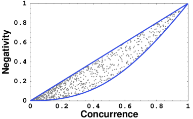
Figure 1: Comparison of negativity and concurrence. Dots represent randomly generated states. (The form of the boundary is discussed in the text.) It is apparent that these two measures of entanglement can give different orderings for pairs of states.

Hence, when we wish to explain maximally entangled mixed states we need to be very explicit about the measure of entanglement (and also mixedness; see the following section). Different measures are likely to lead to different classes of MEMS states.

We end this section by mentioning the three entanglement measures that we shall use to compute the entanglement-mixedness frontiers: entanglement of formation, negativity, and relative entropy of entanglement. The first two of these are straightforward to compute, at least in two-qubit settings. For the third, certain results are available VedralPlenio98 ; Verstraete_Audenaert_deMoor01 that ease the computation of MEMS. We have also reviewed four additional measures (entanglement cost, entanglement of distillation, LS entanglement, and the Bures metric). Of these, however, the first two are rather difficult to compute, let alone maximize; the third is also difficult to compute, at least in practice. As for the fourth, calculating the entanglement involves finding the closest separable states (as is required for the case of relative entropy).

III Measures of mixedness

In the entanglement-measure literature, two measures of mixedness have basically been used: $\big{(}1-{\rm Tr}[\rho^{2}]\big{)}$ and the von Neumann entropy. Whereas the latter has an natural significance stemming from its connections with statistical physics and information theory, the former is substantially easier to calculate. Of course, for density matrices that are almost completely mixed, the two measures show the same trend.

III.1 von Neumann entropy

The von Neumann entropy, the standard measure of randomness of a statistical ensemble described by a density matrix, is defined by

$$S_{\rm V}(\rho)\equiv-\mathrm{Tr}(\rho\log\rho)=-\sum_{i}\lambda_{i}\,\log\lambda_{i}\,,$$ (11)

where $\lambda_{i}$ are the eigenvalues of the density matrix $\rho$ and the $\log$ is taken to base ${\cal N}$, the dimension of the Hilbert space in question. It is straightforward to show that the extremal values of $S_{\rm V}$ are zero (for pure states) and unity (for completely mixed states). To compute the von Neumann entropy it is necessary to have the full knowledge of the eigenvalue spectrum.

As we shall mention in the following subsection, there is a linear entropy threshold above which all states are separable. Qualitatively identical behavior is encountered for the von Neumann entropy. In particular, as we shall see in Sec. IV.3.1, for two-qubit systems all states are separable for $S_{\rm V}\geq-(1/2)\log_{4}(1/12)\approx 0.896$.

III.2 Purity and linear entropy

The second measure that we shall consider is called the linear entropy and is based on the purity of a state, ${\cal P}\equiv{\rm Tr}\left[\rho^{2}\right]$, which ranges from 1 (for a pure state) to $1/{\cal N}$ for a completely mixed state with dimension ${\cal N}$. The linear entropy $S_{\rm L}$ is defined via

$$S_{\rm L}(\rho)\equiv\frac{{\cal N}}{{\cal N}-1}(1-\mbox{Tr}[\rho^{2}]),$$ (12)

which ranges from 0 (for a pure state) to 1 (for a maximally mixed state). The linear entropy is generally a simpler quantity to calculate than the von Neumann entropy as there is no need for diagonalization. For $C^{2}\otimes C^{2}$ systems the linear entropy can be written explicity as

$$S_{\rm L}(\rho)\equiv\frac{4}{3}(1-\mbox{Tr}\left[\rho^{2}\right]).$$ (13)

A related measure, which we shall not use in this Paper (but mention for the sake of completeness), is the inverse participation ratio. Defined via $R\equiv 1/\mbox{Tr}\left[\rho^{2}\right]$, it ranges from $1$ (for a pure state) to ${\cal N}$ (for the maximally mixed state). An attractive property of the inverse participation ratio is that all states with $R\geq{\cal N}-1$ are separable Zyczkowski_Horodecki_Sanpera_Lewenstein98 , which implies all states with a linear entropy $S_{\rm L}(\rho)\geq{\cal N}{({\cal N}-2)}/\left({\cal N}-1\right)^{2}$ (which is $8/9$ when ${\cal N}=4$) are separable.

III.3 Comparing linear and von Neumann entropies

The aim of this subsection is to illustrate the difference between the linear and von Neumann entropies. We shall do this by considering the ${\cal N}=4$ Hilbert space, and seeking the highest and lowest von Neumann entropies consistent with a given value of linear entropy. Before restricting ${\cal N}$ to 4, the corresponding stationarity problem reads:

$$\delta\left(S_{\rm V}(\rho)+\beta\frac{{\cal N}-1}{2{\cal N}}S_{\rm L}(\rho)-(\nu-1)\mbox{Tr}\rho\right)=0,$$ (14)

where $\beta$ and $\nu$ are, respectively, Langrange multipliers that enforce the constraints that linear entropy be fixed and that $\rho$ be normalized. Thus, we arrive at the engaging self-consistency condition

$$\rho=\exp(-\nu-\beta\rho),$$ (15)

in which $\nu$ and $\beta$ can be fixed upon implementing the constraints.

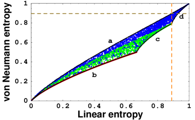
Figure 2: Comparison of linear entropy and von Neumann entropy. Dots represent randomly generated states; pure (Rank-1) states lie at the origin; Rank-2 states lie on segment $b$; the lighter dots in the interior are Rank-3 states; the darker ones are Rank-4 states. The lower boundary comprises three segments meeting at cusps, whereas the upper boundary is a smooth curve. The two dashed lines represent thresholds of entropies beyond which no states contain entanglement.

By hypothesizing certain relationships among the eigenvalues of the density matrix, we have been able, for the case of ${\cal N}=4$, to find certain solutions of the self-consistency condition and, hence, a candidate for the boundary of the region of $S_{\rm L}$ vs. $S_{\rm V}$ plane (see Fig. 2) corresponding to legitimate density matrices. These solutions, when given in terms of eigenvalues, read

$$\Big{\{}\frac{1\!-\!{r}}{4}\!,\frac{1\!-\!{r}}{4}\!,\frac{1\!-\!{r}}{4}\!,\frac{1\!+\!3{r}}{4}\!\Big{\}},\ \mbox{for}\ 0\leq{r}\leq 1,$$ (16a)

$$\{{r},1-{r},0,0\},\qquad\qquad\quad\ \mbox{for}\ \frac{1}{2}\leq{r}\leq 1,$$ (16b)

$$\Big{\{}{r},\frac{1\!-\!{r}}{2},\frac{1\!-\!{r}}{2},0\Big{\}},\ \qquad\quad\mbox{for}\ 0\leq{r}\leq\frac{1}{3},$$ (16c)

$$\Big{\{}\frac{4\!-\!{r}}{12},\frac{4\!-\!{r}}{12},\frac{4\!-\!{r}}{12},\frac{3{r}}{12}\Big{\}},\ \ \ \mbox{for}\ 0\leq{r}\leq 1,$$ (16d)

and they correspond to the upper boundary, and the lowest, middle, and highest pieces of the lower boundary, respectively. Note that the lower boundary comprises three (in general, ${\cal N}-1$) segments that meet at cusps. We remark, parenthetically, that the solutions with zero eigenvalues correspond to extrema within some subspace spanned by those eigenvectors with nonzero eigenvalues, and therefore only obey the stationarity condition (15) within the subspace.

Is there any significance to the boundary states? Boundary segment (a) includes the Werner states defined in Eq. (24). Boundary segment (b) includes the first branch of the MEMS for $E_{\rm F}$ and $S_{\rm L}$ specified below in Eq. (23). The segment (c) includes the states

$$\rho_{c}={r}|\phi^{+}\rangle\langle\phi^{+}|+\frac{1\!-\!{r}}{2}\big{(}|01\rangle\langle 01|\!+\!|10\rangle\langle 10|\big{)}.$$ (17)

States on segment (d) are all unentangled. Of course, the boundary segments include not only the specified states but also all states derivable from them by global unitary transformation.

As for the interior, we have obtained this numerically by constructing a large number of random sets of eigenvalues of legitimate density matrices, and computing for each the two entropies. As Fig. 2 shows, no points lie outside the boundary curve, providing confirmatory evidence for the forms given in Eq. (16).

The fact that the bounded region is two-dimensional indicates the lack of precision with which the linear entropy characterizes the von Neumann entropy (and vice versa, if one wishes). In particular, the figure reveals an ordering difficulty: pairs of states, $A$ and $B$, exist for which $S_{\rm L}^{A}-S_{\rm L}^{B}$ and $S_{\rm V}^{A}-S_{\rm V}^{B}$ differ in sign. Worse still, states having a common value of $S_{\rm V}$ have a continuum of values of $S_{\rm L}$, and vice versa.

IV Entanglement-versus-mixedness frontiers

We now attempt to identify regions in the plane spanned by entanglement and mixedness that are inhabited by physical states (i.e., characterized by legitimate density matrices). We shall consider the various measures of entanglement and mixedness discussed in the previous section. Of particular interest will be the structure of the states that inhabit the frontier, i.e., the boundary delimiting the region of physical states. Frontier states are maximal in the following sense: for a given value of mixedness they are maximally entangled; for a given value of entanglement they are maximally mixed.

IV.1 Parametrization of maximal states

The aim of this subsection is to derive the general form of the maximal states given in Eq. (21), which is what we will use to parametrize maximal states. In Ref. Verstraete_Audenaert_deMoor01 , it is shown that, given a fixed set of eigenvalues, all states that maximize one of the three entanglement measures (entanglement of formation, negativity or relative entropy) automatically maximize the other two. It was further shown that the global unitary transformation that takes arbitrary states into maximal ones has the form

$$U=(U_{1}\otimes U_{2})TD_{\phi}\Phi^{\dagger},$$ (18)

where $U_{1}$ and $U_{2}$ are arbitary local unitary transformations,

$$T\equiv\begin{pmatrix}0&0&0&1\cr\frac{1}{\sqrt{2}}&0&\frac{1}{\sqrt{2}}&0\cr\frac{1}{\sqrt{2}}&0&\frac{-1}{\sqrt{2}}&0\cr 0&1&0&0\cr\end{pmatrix},$$ (19)

$D_{\phi}$ is a unitary diagonal matrix, and $\Phi$ is the unitary matrix that diagonalizes the density matrix $\rho$, i.e., $\rho=\Phi\Lambda\Phi^{\dagger}$, where $\Lambda$ is a diagonal matrix, the diagonal elements of which are the four eigenvalues of $\rho$ listed in nonincreasing order ($\lambda_{1}\geq\lambda_{2}\geq\lambda_{3}\geq\lambda_{4}$). Hence, the general form of a density matrix that is maximal, given a set of eigenvalues, is (up to local unitary transformations)

$$T\begin{pmatrix}\lambda_{1}&0&0&0\cr 0&\lambda_{2}&0&0\cr 0&0&\lambda_{3}&0\cr 0&0&0&\lambda_{4}\cr\end{pmatrix}T^{\dagger}\!=\!\begin{pmatrix}\lambda_{4}\!&\!0\!&\!0\!&\!0\cr 0\!&\!\frac{\lambda_{1}\!+\!\lambda_{3}}{2}\!&\!\frac{\lambda_{1}\!-\!\lambda_{3}}{2}\!&\!0\cr 0\!&\!\frac{\lambda_{1}\!-\!\lambda_{3}}{2}\!&\!\frac{\lambda_{1}\!+\!\lambda_{3}}{2}\!&\!0\cr 0\!&\!0\!&\!0\!&\!\lambda_{2}\cr\end{pmatrix}\!.$$ (20)

This matrix is locally equivalent to the form

$$\begin{pmatrix}x+\frac{{r}}{2}&0&0&\frac{{r}}{2}\cr 0&a&0&0\cr 0&0&b&0\cr\frac{{r}}{2}&0&0&x+\frac{{r}}{2}\cr\end{pmatrix},$$ (21)

with $x\!+\!\frac{{r}}{2}\!=\!(\lambda_{1}\!+\!\lambda_{3})/2$, ${r}\!=\!\lambda_{1}\!-\!\lambda_{3}$, $a\!=\!\lambda_{2}$, and $b\!=\!\lambda_{4}$. The above derivation justifies the Ansatz form (22) used in Ref. Munro_James_White_Kwiat01 to derive the entanglement of formation vs. linear entropy MEMS. We remark that one may as well use the four eigenvalues $\lambda_{i}$’s as the parametrization. Nevertheless, the form (21), as well as (22), can be nicely viewed as a mixture of a Bell state $|\phi^{+}\rangle$ with some diagonal separable mixed state.

IV.2 Entanglement-versus-linear-entropy frontiers

We begin by measuring mixedness in terms of the linear entropy, and comparing the frontier states for various measures of entanglement.

IV.2.1 Entanglement of formation

The characterization of physical states in terms of their entanglement of formation and linear entropy was introduced by Munro et al. in Ref. Munro_James_White_Kwiat01 . (Strictly speaking, they considered the tangle rather than the equivalent entanglement of formation.)  Here, we shall consider yet another equivalent quantity: concurrence (see Sec. II.1). In order to find the frontier, Munro et al. proposed Ansatz states of the form

$$\rho_{\mbox{\tiny Ansatz}}=\begin{pmatrix}x+\frac{{r}}{2}&0&0&\frac{{r}}{2}\cr 0&a&0&0\cr 0&0&b&0\cr\frac{{r}}{2}&0&0&y+\frac{{r}}{2}\cr\end{pmatrix},$$ (22)

where $x,y,a,b,{r}\geq 0$ and $x+y+a+b+{r}=1$. They found that, of these, the subset

$$\rho_{\mbox{\tiny MEMS:$E_{\rm F},S_{\rm L}$}}=\begin{cases}\ \rho_{\rm I}({r}),&{\rm for\ }\frac{2}{3}\leq{r}\leq 1;\cr\ \rho_{\rm I\!I}({r}),&{\rm for\ }0\leq{r}\leq\frac{2}{3};\cr\end{cases}\quad\quad$$ (23a)

$$\rho_{\rm I}({r})\!=\!\begin{pmatrix}\frac{{r}}{2}\!&\!0\!&\!0&\frac{{r}}{2}\cr 0\!&\!1\!\!-\!\!{r}\!&\!0&0\cr 0\!&\!0\!&\!0&0\cr\frac{{r}}{2}\!&\!0\!&\!0&\frac{{r}}{2}\cr\end{pmatrix}\!,\ \rho_{\rm I\!I}({r})\!=\!\begin{pmatrix}\frac{1}{3}&0&0&\frac{{r}}{2}\cr 0&\frac{1}{3}&0&0\cr 0&0&0&0\cr\frac{{r}}{2}&0&0&\frac{1}{3}\cr\end{pmatrix}\!,$$ (23b)

lies on the boundary in the tangle vs. linear-entropy plane and, accordingly, named these MEMS, in the sense that these states have maximal tangle for a given linear entropy. We remark that at the crossing point of the two branches, ${r}=2/3$, the density matrices on either side coincide.

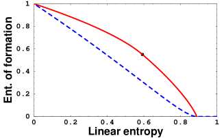
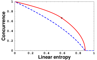
Figure 3: Entanglement frontier. Upper panel: entanglement of formation vs. linear entropy. Lower panel: concurrence vs. linear entropy. The states on the boundary (solid curve) are $\rho_{\mathrm{MEMS};E_{\rm F},S_{\rm L}}$. A dot indicates a transition from one branch of MEMS to another. The dashed curve below the boundary contains Werner states.

In Fig. 3 we plot the entanglement of formation/concurrence vs. linear entropy for the family of MEMS (23); this gives the frontier curve. For the sake of comparison, we also give the curve associated with the family of Werner states of the form

$$\rho_{\rm W}\equiv{r}|\phi^{+}\rangle\langle\phi^{+}|\!+\!\frac{1-{r}}{4}\openone=\begin{pmatrix}\frac{1+{r}}{4}&0&0&\frac{{r}}{2}\cr 0&\frac{1-{r}}{4}&0&0\cr 0&0&\frac{1-{r}}{4}&0\cr\frac{{r}}{2}&0&0&\frac{1+{r}}{4}\end{pmatrix}.$$ (24)

Evidently, for a given value of linear entropy these MEMS (which we shall denote by $\{{\rm MEMS}\!:\!E_{\rm F},S_{\rm L}\}$) achieve the highest concurrence. As the tangle $\tau$ and entanglement of formation $E_{\rm F}$ are monotonic functions of the concurrence, Eq. (23) also gives the boundary curve for these measures. This raises an interesting question: Is (23) optimal for other measures of entanglement?

IV.2.2 Relative entropy as the entanglement measure

To find the frontier states for the relative entropy of entanglement we again turn our attention to the maximal density matrix (21). For this form of density matrix the linear entropy is given (with $x$ expressed in terms of $a,b,{r}$) by

$$S_{\rm L}=\frac{2}{3}\!\left(-3a^{2}+2a\left(1\!-\!b\right)+\left(1\!-\!b\right)\left(1\!+\!3b\right)\!-\!{r}^{2}\right)\!.$$ (25)

To calculate the relative entropy of entanglement, we need to determine the closest separable state to (21). It is simpler to do this analysis via several cases. We begin by considering the Rank-2 and Rank-3 cases of (21). We set $b=0$ ($\lambda_{4}=0$) and express $x$ in terms of $a$ and ${r}$ in the density matrix, obtaining

$$\rho=\begin{pmatrix}\frac{1-a}{2}&0&0&\frac{{r}}{2}\cr 0&a&0&0\cr 0&0&0&0\cr\frac{{r}}{2}&0&0&\frac{1-a}{2}\end{pmatrix},$$ (26)

and thus find that the closest separable density matrix $\sigma^{*}$ is given by VedralPlenio98

$$\sigma^{\ast} = \begin{pmatrix}C&0&0&D\cr 0&E&0&0\cr 0&0&1\!-\!2C\!-\!E&0\cr D&0&0&C\cr\end{pmatrix},$$ (27a)

$$C \equiv \frac{\left(1\!+\!a\right)\left(1\!-\!a^{2}\!-\!{r}^{2}\right)}{2\left(1\!+\!a\!-\!{r}\right)\left(1\!+\!a\!+\!{r}\right)},$$ (27b)

$$D \equiv \frac{a\left(1\!+\!a\right){r}}{\left(1\!+\!a\!-\!{r}\right)\left(1\!+\!a\!+\!{r}\right)},$$ (27c)

$$E \equiv \frac{a\left(1\!+\!a\right)^{2}}{\left(1\!+\!a\!-\!{r}\right)\left(1\!+\!a\!+\!{r}\right)}.$$ (27d)

The relative entropy of entanglement is now simply given by

$$E_{\rm R}(\rho)={\rm Tr}\left(\rho\log\rho-\rho\log\sigma^{\ast}\right)$$

$$\quad=\!\frac{1\!+\!a}{2}\log\frac{(1\!+\!a)^{2}\!-\!{r}^{2}}{(1\!+\!a)^{2}}+\frac{{r}}{2}\log\frac{1\!+\!a\!+\!{r}}{1\!+\!a\!-\!{r}},$$ (28)

with the linear entropy being given by

$$S_{\rm L}\!=\!\frac{2}{3}\!\left(1\!+\!2a\!-\!3a^{2}-\!{r}^{2}\right),$$ (29)

subject to the constraint $(a+{r})\leq 1$. For the Rank-2 case $a=1-{r}$ ($b=x=0$), and the resulting solution is the Rank-2 matrix $\rho_{\rm I}({r})$ given in Eq. (23) with $1/2\leq{r}\leq 1$. We remark that this Rank-2 solution is always a candidate MEMS for the three entanglement measures that we consider in this Paper. In order to determine whether or in what range the Rank-2 solution achieves the global maximum, we need to compare it with the Rank-3 and Rank-4 solutions.

By maximizing $E_{\rm R}(\rho)$ for a given value of $S_{\rm L}$, we find the following stationary condition:

$${r}\log\frac{(1+a)^{2}-{r}^{2}}{(1+a)^{2}}=(3a-1)\log\frac{1+a+{r}}{1+a-{r}}.$$ (30)

Given a value of $S_{\rm L}$, we can solve Eqs. (29) and (30), at least numerically, to obtain the parameters $a$ and ${r}$, and hence, from Eq. (26), the Rank-3 MEMS. However, if the constraint inequality $a+{r}\leq 1$ turns out to be violated, the solution is invalid.

We now turn to the Rank-4 case. It is straightforward, if tedious, to show that the Werner states, Eq. (24), obey the stationarity conditions appropriate for Rank 4. However, it turns out that this solution is not maximal.

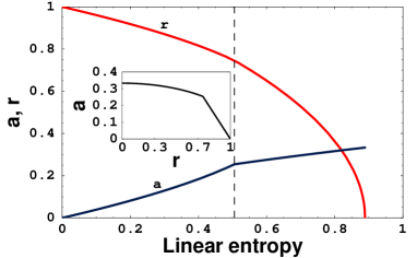
Figure 4: Dependence of $a$ and ${r}$ of the frontier states on linear entropy. The dotted line indicates the transition between two branches of MEMS.

To summarize, the frontier states, which we denote by $\{{\rm MEMS}\!:\!E_{\rm R},S_{\rm L}\}$, are states of the form (26); the dependence of the parameters $a$ and ${r}$ on $S_{\rm L}$ is shown in Fig. 4. In Fig. 5, we show the resulting frontier, as well as curves corresponding to non-maximal stationary states. The frontier states have the following structure: (i) for $S_{\rm L}\lesssim 0.5054$ they are the Rank-2 MEMS of Eq. (23) but with ${r}$ restricted to the range from $1$ (at $S_{\rm L}=0$) to approximately $0.7459$ (at $S_{\rm L}\simeq 0.5054$); (ii) for $S_{\rm L}\gtrsim 0.5054$ the MEMS are Rank 3, with parameters $a$ and ${r}$ satisfying Eqs. (30) and (29) at each value of $S_{\rm L}$, and $(a,{r})$ ranging between approximately $(0.3056,0.7459)$ (at $S_{\rm L}\simeq 0.5054$) and $(1/3,0)$ (at $S_{\rm L}=8/9$). As noted previously, beyond $S_{\rm L}=8/9$ there are no entangled states. As the inset of Fig. 4 shows, the parameter $a$ can be regarded as a continous function of parameter ${r}\in[0,1]$. The two branches of the solution, (i) and (ii), cross at $(S^{*}_{\rm L},E^{*}_{\rm R})\simeq(0.5054,0.3422)$; at this point, the states on the two branches coincide,

$$\rho^{*}\simeq\begin{pmatrix}0.372947&0&0&0.372947\cr 0&0.254106&0&0\cr 0&0&0&0\cr 0.372947&0&0&0.372947\end{pmatrix}.$$ (31)

Just as in the case of entanglement of formation vs. linear entropy, the density matrix is continuous at the transition between branches.

We remark that the curve generated by the states $\{{\rm MEMS}\!:\!E_{\rm F},S_{\rm L}\}$, when plotted on the $E_{\rm R}$ vs. $S_{\rm L}$ plane, falls just slightly below that generated by the states $\{{\rm MEMS}\!:\!E_{\rm R},S_{\rm L}\}$ for $S_{\rm L}\gtrsim 0.5054$ (and coincides for smaller values of $S_{\rm L}$).

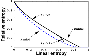
Figure 5: Entanglement frontier: relative entropy of entanglement vs. linear entropy. The frontier states (solid curve) are $\rho_{\mathrm{MEMS};E_{\rm R},S_{\rm L}}$. The dot indicates the transition between branches of MEMS.

We also remark that the parameter ${r}$ turns out to be the concurrence $C$ of the states, so that Fig. 4 can be interpreted a plot of the concurrence of the frontier states vs. their linear entropy. By comparing this concurrence vs. linear entropy curve to that in Fig. 3, we find that the former lies just slightly below the latter for $S_{\rm L}\gtrsim 0.5054$ (and the two coincide for smaller values of $S_{\rm L}$), the maximal difference between the two being less than $10^{-2}$.

It is evident that, for a given linear entropy, the relative entropies of entanglement for both $\{{\mathrm{MEMS}\!:\!E_{\rm R},S_{\rm L}}\}$ and $\{{\mathrm{MEMS}\!:\!E_{\rm F},S_{\rm L}}\}$ are significantly less than the corresponding entanglements of formation. In fact, for small degrees of impurity, the entanglements of formation for the two MEMS states are quite flat; however, the relative entropies of entanglement fall quite rapidly. More specifically, for a change in linear entropy of $\Delta S_{\rm L}=0.1$ near $S_{\rm L}=0$ we have that $\Delta E_{\rm F}\approx 0.05$ (see Fig. 3) and $\Delta E_{R}\approx 0.2$ (see Fig. 5). As the curves of the states $\{{\rm MEMS}\!:\!E_{\rm F},S_{\rm L}\}$ and $\{{\rm MEMS}\!:\!E_{\rm R},S_{\rm L}\}$ are very close on the two planes, $E_{\rm F}$ vs. $S_{\rm L}$ and $E_{\rm R}$ vs. $S_{\rm L}$, we show, in Fig. 6, the entanglement difference $E_{\rm F}-E_{\rm R}$ for the states $\{{\rm MEMS}\!:\!E_{\rm F},S_{\rm L}\}$, and compare it with the corresponding difference for the Werner states. While it is clear that $E_{\rm R}(\rho)\leq E_{\rm F}(\rho)$, for certain values of the linear entropy the difference turns out to be quite large, this difference being uniformly larger for $\{{\rm MEMS}\!:\!E_{\rm F},S_{\rm L}\}$ than for the Werner state; see Fig. 6. This raises several interesting questions, e.g., whether, for a given value of $E_{\rm F}$, the undistillable entanglement (the difference between the entanglement of formation and the relative entropy of entanglement is the lower bound) increases as states become more mixed.

Figure 6: Difference in entanglement ($E_{\rm F}-E_{\rm R}$) vs. $S_{\rm L}$ for the MEMS in Eq. (23) and Werner states. The solid curve shows states from $\rho_{\mathrm{MEMS};E_{\rm F},S_{\rm L}}$; the dashed curve shows the Werner states.

As we have seen, Werner states are not frontier states either in the case of entanglement of formation or in the case of relative entropy of entanglement. By contrast, as we shall see in the next section, if we measure entanglement via negativity, then for a given amount of linear entropy, the Werner states (as well as another Rank-3 class of states) achieve the largest value of entanglement. Said equivalently, the Werner states belong to $\{{\rm MEMS\!:\!N,S_{\rm L}}\}$.

IV.2.3 Negativity

In order to derive the form of the MEMS in the case of negativity, we again consider the density matrix of the form (21), for which it is straightforward to show that the negativity $N$ is given by

$$N=\max\{0,\sqrt{(a-b)^{2}+{r}^{2}}-(a+b)\}.$$ (32)

Furthermore, because we aim to find the entanglement frontier, we can simply restrict our attention to states satisfying $N>0$, i.e., to states that are entangled Peres96_Horodecki396 . Then, by making $N$ stationary at fixed $S_{\rm L}$ and with the constraint $2x+a+b+{r}=1$, we find two one-parameter families of stationary states (in addition to the Rank-2 MEMS, which are common to all three entanglement measures). The parameters of the first family obey

$$a=b=x,\ {r}=1-4x.$$ (33)

When expressed in terms of parameter ${r}$, the density matrix takes the form

$$\rho^{(1)}_{\mbox{\tiny MEMS:$N\!,\!S_{\rm L}$}}=\begin{pmatrix}\frac{1+{r}}{4}&0&0&\frac{{r}}{2}\cr 0&\frac{1-{r}}{4}&0&0\cr 0&0&\frac{1-{r}}{4}&0\cr\frac{{r}}{2}&0&0&\frac{1+{r}}{4}\end{pmatrix},$$ (34)

which are precisely the Werner states in Eq. (24). For the second solution, the parameters obey

$$a\!=\!\frac{4\!-\!2\sqrt{3{r}^{2}\!+\!1}}{6},b\!=\!0,x\!=\!\frac{1\!+\!\sqrt{3{r}^{2}\!+\!1}}{6}\!-\!\frac{{r}}{2}.$$ (35)

When expressed in terms of parameter ${r}$, the density matrix takes the form

$$\rho^{(2)}_{\mbox{\tiny MEMS:$N\!,\!S_{\rm L}$}}\!=\!\begin{pmatrix}\frac{1+\sqrt{3{r}^{2}\!+\!1}}{6}\!\!&\!\!0\!&\!0\!\!&\frac{{r}}{2}\cr 0\!\!&\!\!\frac{4-2\sqrt{3{r}^{2}\!+\!1}}{6}\!&\!0\!\!&0\cr 0\!\!&\!\!0\!&\!0\!\!&0\cr\frac{{r}}{2}\!\!&\!\!0\!&\!0\!\!&\frac{1+\sqrt{3{r}^{2}\!+\!1}}{6}\end{pmatrix}\!.$$ (36)

We remark that the two solutions give the same bound on the negativity for a given value of linear entropy. The resulting frontier in the negativity vs. linear entropy plane is shown in Fig. 7.

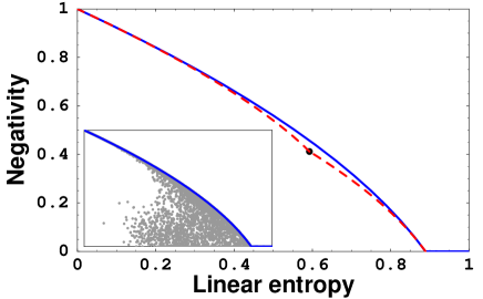
Figure 7: Entanglement frontier: negativity vs. linear entropy. States on the boundary (full line) are $\rho^{(1)}_{{\rm MEMS}:N,S_{\rm L}}$ and $\rho^{(2)}_{{\rm MEMS}:N,S_{\rm L}}$. The dashed line comprises $\rho_{{\rm MEMS}:E_{\rm F},S_{\rm L}}$. Inset: the randomly generated states confirm the location of the frontier.

We have shown by numerical exploration FOOT:NSL that the family states found in the previous paragraph do indeed achieve the maximal negativity. The results of this exploration are indicated by points in the inset in Fig. 7, and compelling evidence for the maximality of the negativity is furnished by the fact that no points lie beyond the frontier.

Thus, the states $\{{\rm MEMS}\!:\!N,S_{\rm L}\}$ on the boundary include, up to local unitary transformations, both Werner states in Eq. (34) and states in Eq. (36). We also plot in Fig. 7 the curve belonging to $\{{\rm MEMS}\!:\!E_{\rm F},S_{\rm L}\}$; note that it falls slightly below the curve associated with $\{{\rm MEMS}\!:\!N,S_{\rm L}\}$ and that it has a cusp, due to the structure of the states, at the value $2/3$ for the parameter ${r}$ in Eq. (23). Here, we see that maximally entangled mixed states change their form when we adopt a different entanglement measure.

IV.3 Entanglement-versus-von-Neumann-entropy frontiers

We continue this section by choosing to measure mixedness in terms of the von Neumann entropy, and comparing the frontier states for various measures of entanglement.

IV.3.1 Entanglement of formation

To find this frontier, we consider states of the form (21), and compute for them the concurrence and the von Neumann entropy:

$$\!\!\!\!\!\!\!\!\!\!\!\!\!C\!\!\! = \!\!\!{r}-2\sqrt{ab},$$ (37a)

$$\!\!\!\!\!\!\!\!\!\!\!\!\!S_{\rm V}\!\!\! = \!\!\!-a\log a\!-\!b\log b\!-\!x\log x\!-\!(x\!\!+\!\!{r})\log(x\!\!+\!\!{r}).$$ (37b)

Note that the parameters obey the normalization constraint $2x\!+\!a\!+\!b\!+\!{r}=1$.

As we remarked previously, the Rank 2 MEMS is always a candidate. For the Rank-3 case, we can set $b=0$ in Eq. (37). By maximizing $C$ at fixed $S_{\rm V}$, we find a stationary solution:
(i) ${r}=C$, $x=(4\!-\!3C\!-\!\sqrt{4\!-\!3C^{2}})/6$, and $a=(\sqrt{4\!-\!3C^{2}}\!-\!1)/3$; the resulting density matrix is

$$\rho_{\rm i}=\begin{pmatrix}\frac{4-\sqrt{4-3C^{2}}}{6}\!&\!0\!&\!0&\frac{C}{2}\cr 0\!&\!\frac{\sqrt{4-3C^{2}}-1}{3}\!&\!0&0\cr 0\!&\!0\!&\!0&0\cr\frac{C}{2}\!&\!0\!&\!0&\frac{4-\sqrt{4-3C^{2}}}{6}\cr\end{pmatrix}\!.$$ (38)

For the Rank-4 case ($b\neq 0$), the stationarity condition can be shown to be

$$u\log(u) = w\log(w),$$ (39a)

$$2u\log(u) = (u+w)\log(v),$$ (39b)

where $u\equiv\sqrt{a/(x\!+\!{r})}$, $v\equiv\sqrt{x/(x\!+\!{r})}$, and $w\equiv\sqrt{b/(x\!+\!{r})}$. There are two solutions, due to the two-to-one property of the function $z\log z$ for $z\in(0,1)$. The first one is ($u=v=w$).
(ii) $a=b=x=(1\!-\!C)/6$, and ${r}=(1\!+\!2C)/3$, which can readily be seen to be a Werner state as in Eq. (24) or, equivalently,

$$\rho_{\rm ii}=\begin{pmatrix}\frac{2+C}{6}&0&0&\frac{1+2C}{6}\cr 0&\frac{1-C}{6}&0&0\cr 0&0&\frac{1-C}{6}&0\cr\frac{1+2C}{6}&0&0&\frac{2+C}{6}\cr\end{pmatrix}.$$ (40)

Being the concurrence, $C$ is restricted to the interval $[0,1]$. The second solution is transcendental, but can be solved numerically.

In Fig. 8 we compare the four possible candidate solutions, and find that the global maximum is composed of only (i) and (ii).

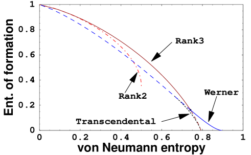
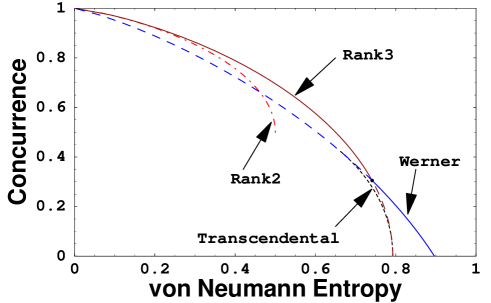
Figure 8: Entanglement frontiers. Upper panel: entanglement of formation vs. von Neumann entropy. Lower panel: concurrence vs. von Neumann entropy. The branch structure is described in the text.

We summarize the states at the frontier as follows:

$$\rho_{\mathrm{MEMS}:E_{\rm F},S_{\rm V}}=\begin{cases}\rho_{\rm ii},&{\rm for}\ 0\leq C\leq C^{*};\cr\rho_{\rm i},&{\rm for}\ C^{*}\leq C\leq 1.\cr\end{cases}$$ (41)

Note the crossing point at $\big{(}C,S_{\rm V}\big{)}=\big{(}C^{*},S_{\rm V}(C^{*})\big{)}$, at which extremality is exchanged, so the true frontier consists of two branches. It is readily seen that $C^{*}$ is the solution of the equation $S_{\rm V}(\rho_{\rm i}(C))=S_{\rm V}(\rho_{\rm ii}(C))$, and the approximate numerical values of $C^{*}$ and the corresponding $S_{\rm V}^{*}$ are $0.305$ and $0.741$, respectively.

The resulting form of MEMS states is peculiar, in that, even at the crossing point of two branches on the entanglement-mixedness plane, the forms of matrices on the two branches are not equivalent (one is Rank 3, the other Rank 4). This is in contrast to the $\{{\rm MEMS}\!:\!E_{\rm F},S_{\rm L}\}$. This peculiarity can be partially understood from the plot of the two mixedness measures, Fig. 2: as the value of the von Neumann entropy rises, there are fewer and fewer Rank-3 entangled states, and above some threshold, no more Rank-3 states exist, let alone entangled Rank-3 states. There are, however, still entangled states of Rank 4. Hence, if Rank-3 states attain higher entanglement than Rank-4 states do when the entropy is low, a transition must occur between MEMS states of Rank 3 and Rank 4.

From Fig. 8 it is evident that beyond a certain value of the von Neumann entropy no entangled states exist. This value can be readily obtained by considering the MEMS state (40) at $C=0$,

$$\begin{pmatrix}\frac{1}{3}&0&0&\frac{1}{6}\cr 0&\frac{1}{6}&0&0\cr 0&0&\frac{1}{6}&0\cr\frac{1}{6}&0&0&\frac{1}{3}\cr\end{pmatrix},$$ (42)

for which $S_{\rm V}=-(1/2)\log_{4}(1/12)\approx 0.896$.

As an aside, we mention a tantalizing but not yet fully developed analogy with thermodynamics Horodecki398 . In this analogy, one associates entanglement with energy and von Neumann entropy with entropy, and it is therefore tempting to regard the MEMS just derived as the analog of thermodynamic equilibrium states. If we apply the Jaynes principle to an ensemble in equilibrium with a given amount of entanglement then the most probable states are those MEMS shown above.

IV.3.2 Relative entropy of entanglement

Let us now find the frontier states for the case of relative entropy of entanglement. To do this, we first consider the Rank-3 states in Eq. (26), for which the relative entropy is given by Eq. (IV.2.2). For these states, the von Neumann entropy is given by

$$S_{\rm V}\!=\!-\frac{1\!\!-\!\!a\!\!+\!\!{r}}{2}\!\log\!\!\frac{1\!\!-\!\!a\!\!+\!\!{r}}{2}-a\log a-\frac{1\!\!-\!\!a\!\!-\!\!{r}}{2}\!\log\!\!\frac{1\!\!-\!\!a\!\!-\!\!{r}}{2},$$ (43)

where the $\log$ function is taken to be base four. Even though the $\log$ functions in $S_{\rm V}$ and $E_{\rm R}$ use different bases, the stationary condition for the parameters ${r}$ and $a$ does not change, because the difference can be absorbed by a rescaling of the constraint-enforcing Lagrange multiplier. Thus, in maximizing $E_{\rm R}$ at fixed $S_{\rm V}$, we arrive at the stationarity condition

$$\log\!\frac{(\!1\!\!+\!\!a\!)^{2}\!-\!{r}^{2}}{(\!1\!\!+\!\!a\!)^{2}}\log\!\frac{1\!\!-\!\!a\!\!-\!\!{r}}{1\!\!-\!\!a\!\!+\!\!{r}}\!=\!\log\!\frac{1\!\!+\!\!a\!\!+\!\!{r}}{1\!\!+\!\!a\!\!-\!\!{r}}\log\!\frac{(\!1\!\!-\!\!a\!)^{2}\!-\!{r}^{2}}{4a^{2}}.$$ (44)

We can solve for the parameter $a$ as a function of $r\in[0,1]$, at least numerically; the result is shown in Fig. 9, along with $S_{\rm V}$ and $E_{\rm R}$.

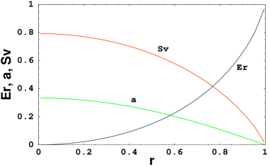
Figure 9: Dependence of $E_{\rm R}$, $S_{\rm V}$ and $a$ on ${r}$ for the Rank-3 maximal states.

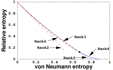
Figure 10: Entanglement frontier: relative entropy of entanglement vs. von Neumann entropy. The solid curve is the frontier. The branch structure is described in the text.

Turning to the Rank-4 case, it is straightforward, if tedious, to show that the Werner states satisfy the corresponding stationarity conditions. In order to ascertain which rank gives the MEMS for a given $S_{\rm V}$, we compare the stationary states of Rank 2, 3, and 4 in Fig. 10. Thus, we see that for $S_{\rm V}\leq S^{*}_{\rm V}\simeq 0.672$ the frontier states are given by the Rank-3 states, whereas for $S_{\rm V}\geq S_{\rm V}^{*}$ the frontier states are given by the Werner states (24) with the parameter ${r}$ ranging from approximately 0.6059 down to 0. At the crossing point, $(S^{*}_{\rm V},E_{\rm R}^{*})\simeq(0.672,0.124)$, the MEMS undergo a discontinuous transition; recall that we encountered a similar phenomenon in the case of entanglement of formation vs. von Neumann entropy.

IV.3.3 Negativity

We saw in Sec. IV.2.3 that there is a pair of families of MEMS which differ in rank but give the identical frontier in the $N$ vs. $S_{\rm L}$ plane. It is interesting to see what happens for the combination of negativity and von Neumann entropy.

Once again, we begin with states of form (21), for which the negativity and the von Neumann entropy are given in Eqs. (32) and (37b), respectively. By making $N$ stationary at fixed $S_{\rm V}$, we are able to find only one solution (in addition to the Rank-2 candidate): $a=b=x$. Expressing the resulting density matrix, as we may, in terms of the single parameter ${r}$, we arrive at the following candidate for the frontier states:

$$\rho_{{\rm MEMS}:N,S_{\rm V}}=\begin{pmatrix}\frac{1+{r}}{4}&0&0&\frac{{r}}{2}\cr 0&\frac{1-{r}}{4}&0&0\cr 0&0&\frac{1-{r}}{4}&0\cr\frac{{r}}{2}&0&0&\frac{1+{r}}{4}\end{pmatrix},$$ (45)

where $0\leq{r}\leq 1$, i.e., the Werner states.

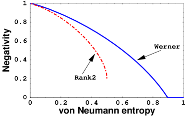
Figure 11: Entanglement frontier: negativity vs. von Neumann entropy. The solid curve is the frontier. The broken curve represents the Rank-2 candidate states.

The resulting frontier in the negativity vs. von-Neumann-entropy plane is shown in Fig. 11 which, for comparison, also shows the curve for the Rank-2 candidate.

V Concluding Remarks

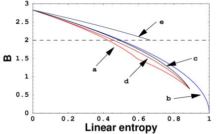
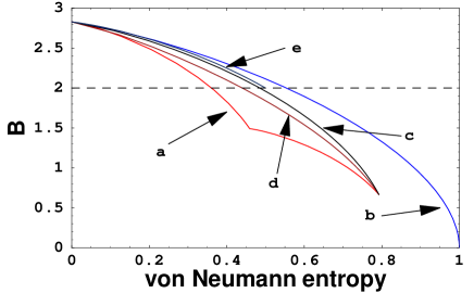
Figure 12: Violation of Bell’s inequality for various families of states: (a) $\{{\rm MEMS}\!:\!E_{\rm F},S_{\rm L}\}$, (b) Werner states, (c) $\rho^{(2)}_{\mbox{\tiny MEMS:$N\!,\!S_{\rm L}$}}$, (d) $\rho_{\rm i}$ in Eq. (38), and (e) the Rank-2 Bell diagonal states in Eq. (48).

In this Paper we have determined families of maximally entangled mixed states (MEMS, i.e., frontier states, which possess the maximum amount of entanglement for a given degree of mixedness). These states may be useful in quantum information processing in the presence of noise, as they have the maximum amount of entanglement possible for a given mixedness. We considered various measures of entanglement (entanglement of formation, relative entropy, and negativity) and mixedness (linear entropy and von Neumann entropy).

We found that the form of the MEMS depends heavily on the measures used. Certain classes of frontier states (such as those arising with either entanglement of formation or relative entropy of entanglement vs. the von Neumann entropy) behave discontinously at a specific point on the entanglement-mixedness frontier. Under most of the settings considered, we have been able to explicitly derive analytical forms for the frontier states.

For entanglement of formation and relative entropyand for most values of mixedness, we have found that the Rank-2 and Rank-3 MEMS have more entanglement than Werner states do. On the other hand, at fixed entropy no states have higher negativity than Werner states do. At small amounts of mixedness, the $\{{\rm MEMS}\!:\!E_{\rm F},S_{\rm L}\}$ states “lose” entanglement with increasing mixedness at a substantially lower rate than do the Werner states. However, when the entanglement is measured by the relative entropy, the difference in loss-rate is significantly smaller.

From Eq. (10) it is tempting to assert that in the case of LS entanglement vs. mixedness the frontier states should be the same as those in the case of entanglement of formation vs. mixedness. However, as we do not know whether Eq. (22) (up to local unitary transformations) exhausts all maximal states for LS entanglement, further investigation of this point is needed.

Having characterized the MEMS for various measures, it is worthwhile considering them from the perspective of Bell-inequality violations. To quantify the violation of Bell’s inequality, it is useful to consider the quantity

$$B\equiv\max_{\vec{a},\vec{a}^{\prime},\vec{b},\vec{b}^{\prime}}\big{\{}E(\vec{a},\vec{b})+E(\vec{a},\vec{b}^{\prime})+E(\vec{a}^{\prime},\vec{b})-E(\vec{a}^{\prime},\vec{b}^{\prime})\big{\}},$$ (46)

where $E(\vec{a},\vec{b})\equiv\langle\vec{\sigma}\cdot\vec{a}\otimes\vec{\sigma}\cdot\vec{b}\rangle$ and the vectors $\vec{a}$ and $\vec{a}^{\prime}$ ($\vec{b}$ and $\vec{b}^{\prime}$) are two different measuring apparatus settings for observer A (observer B). If $B>2$ then the corresponding state violates Bell’s inequality. For the density matrix of the form (21) it is straightforward Aravind95 to show that the quantity $B$ is given by

$$B=2\sqrt{\Big{(}4(x+\frac{{r}}{2})-1\Big{)}^{2}+{r}^{2}}.$$ (47)

In Fig. 12, we plot $B$ vs. linear and von Neumann entropies for several families of frontier states. As a comparison, we also draw the violation by the following Rank-2 state (which is diagonal in the Bell basis):

$$\rho_{\rm B}\equiv{r}|\phi^{+}\rangle\langle\phi^{+}|+(1-{r})|\phi^{-}\rangle\langle\phi^{-}|,\ {r}\in[0,1].$$ (48)

This state, although not belonging to any of the families of frontier states derived previously, turns out to achieve the maximum possible violation, as a function of linear entropy. On the other hand, the Werner states appear to achieve maximal violation in the case of von Neumann entropy. Ekert’s application of Bell’s inequalities to quantum cryptography Ekert91 , together with the discussions of the present paragraph, suggests that MEMS may be relevant to quantum communication.

Another natural application for which entanglement is known to be a critical resource is quantum teleportation. How do these frontier MEMS teleport, compared with the Werner and Rank-2 Bell diagonal states? If we restrict our attention to high purity situations (i.e., to states with only a small amount of mixedness) then it is straightforward to show that, e.g., $\{{\rm MEMS}\!:\!E_{\rm F},S_{\rm L}\}$ states teleport average states better than the Werner states do, but worse than the Rank-2 Bell diagonal state does. Part of the explanation for this behavior is that standard teleportation is optimized for using Bell states as its core resource.

It is also interesting to note that for certain combinations of entanglement and mixedness measures, as well as the Bell inequality violation, the Rank-2 candidates fail to furnish MEMS. Thus, these states seem to be less useful than other MEMS. However, from the perspective of distillation, these states are exactly quasi-distillable Horodecki399 ; VerstraeteDehaeneDeMoor01 , and can be useful in the presence of noise because they can be easily distilled into Bell states.

Appendix A Number of negative eigenvalues of the partial transpose of $\rho$

In this appendix we address the result that for $C^{2}\otimes C^{2}$ systems the partial transpose of any density matrix $\rho$ has at most one negative eigenvalue. In fact, we shall consider the result from two perspectives.

First, we build upon results (Theorem 3, in particular) contained in Ref. VerstraeteDehaeneDeMoor01 , from which it follows that it is sufficient to consider (i) Bell diagonal states and (ii) states of the form

$$\begin{pmatrix}a+c&0&0&d\cr 0&0&0&0\cr 0&0&b-c&0\cr d&0&0&a-b\end{pmatrix}.$$ (49)

For the latter case, straightforward calculation shows that the partially transposed matrix can have one negative eigenvalue when $d\neq 0$ and that it does not have negative eigenvalues when $d=0$. For the former case, suppose that the Bell diagonal state has the four eigenvalues $\lambda_{1}$, $\lambda_{2}$, $\lambda_{3}$, $\lambda_{4}$, in nonincreasing order. Then it is straightforward to see that the corresponding partially transposed matrix has the four eigenvalues $(\lambda_{1}+\lambda_{2}+\lambda_{3}-\lambda_{4})/2$, $(\lambda_{1}+\lambda_{2}-\lambda_{3}+\lambda_{4})/2$, $(\lambda_{1}-\lambda_{2}+\lambda_{3}+\lambda_{4})/2$, $(-\lambda_{1}+\lambda_{2}+\lambda_{3}+\lambda_{4})/2$. Thus, it can have at most one negative eigenvalue.

A second perspective is provided by first invoking the LS decomposition (8) and then making a Schmidt decomposition, via the local unitary transformation $U_{A}\otimes U_{B}$, of the pure entangled part $|\psi_{e}\rangle$. In this way, the pure part becomes

$$U_{A}\otimes U_{B}|\psi_{e}\rangle=\sqrt{p}|00\rangle+\sqrt{1-p}|11\rangle,$$ (50)

where $1/2\leq p\leq 1$. Meanwhile, $\rho$ is transformed into

$$\rho^{\prime} = (U_{A}\otimes U_{B})\ \rho\ (U_{A}^{\dagger}\otimes U_{B}^{\dagger})$$ (51)

$$= \lambda\rho_{s}^{\prime}\!+\!(1\!-\!\lambda)\!\!\begin{pmatrix}\!p\!&\!0\!&\!0\!&\!\sqrt{p(1\!-\!p)}\!\cr\!0\!&\!0\!&\!0\!&\!0\!\cr\!0\!&\!0\!&\!0\!&\!0\!\cr\!\sqrt{p(1\!-\!p)}\!&\!0\!&\!0\!&\!1\!-\!p\!\cr\end{pmatrix},$$

where $\rho_{s}^{\prime}\equiv U_{A}\otimes U_{B}\,\rho_{s}\,U_{A}^{\dagger}\otimes U_{B}^{\dagger}$ is still separable, and its partial transpose remains positive semi-definite.

Taking, then, the partial transpose, the density matrix is transformed into

$${\rho^{\prime}}^{{\rm T}_{B}}\!\!=\!\lambda{\rho_{s}^{\prime}}^{{\rm T}_{B}}\!\!+\!(1\!\!-\!\!\lambda)\!\begin{pmatrix}p\!&\!\!0\!\!&\!\!0\!\!&\!\!0\cr 0\!&\!\!0\!\!&\!\!\sqrt{p(1\!-\!p)}\!\!&\!\!0\cr 0\!&\!\!\sqrt{p(1\!-\!p)}\!\!&\!\!0\!\!&\!\!0\cr 0\!&\!\!0\!\!&\!\!0\!\!&\!\!1\!-\!p\cr\end{pmatrix}\!,$$ (52)

and we note that the last matrix has eigenvalues $\lambda_{1}\!=\!p$, $\lambda_{2}\!=\!\sqrt{p(1\!-\!p)}$, $\lambda_{3}\!=\!1\!-\!p$, $\lambda_{4}\!=\!-\sqrt{p(1\!-\!p)}$ in (as $p\geq 1/2$) nonincreasing order. As the Hermitian matrix ${\rho_{s}^{\prime}}^{{\rm T}_{B}}$ retains positive-semi-definiteness, we can employ a well-known result in matrix analysis Horn_Johnson that for $n\times n$ Hermitian matrices $A$ and $B$, with $B$ being positive semi-definite, the eigenvalues of $(A+B)$ and $A$, when arranged in non-ascending order, obey

$$\lambda_{k}(A+B)\geq\lambda_{k}(A)\quad\mbox{for}\ k=1,2,\ldots,n.$$ (53)

Hence, identifying $B$ with $\lambda{\rho_{s}^{\prime}}^{{\rm T}_{B}}$ and $A$ with the product of $(1\!-\!\lambda)$ and the matrix in Eq. (52), we immediately see that $\lambda_{1}({\rho^{\prime}}^{{\rm T}_{B}})\geq\lambda_{2}({\rho^{\prime}}^{{\rm T}_{B}})\geq\lambda_{3}({\rho^{\prime}}^{{\rm T}_{B}})\geq(1-\lambda)(1-p)\geq 0$ and, thus, ${\rho^{\prime}}^{{\rm T}_{B}}$ (or equivalently ${\rho}^{{\rm T}_{B}}$) can have at most one negative eigenvalue. Thus, the negativity for $C^{2}\otimes C^{2}$ systems can then be written as $N=2\max\{0,-\lambda_{4}(\rho^{{\rm T}_{B}})\}$.

References

- (1) B. Schumacher, Phys. Rev. A 54, 2614 (1996).
- (2) A. K. Ekert, Phys. Rev. Lett. 67, 661 (1991).
- (3) C. H. Bennett, G. Brassard, C. Crépeau, R. Jozsa, A. Peres, and W. K. Wootters, Phys. Rev. Lett. 70, 1895 (1993).
- (4) S. Lloyd, Science 261 1589 (1993); D. P. DiVincenzo, Science 270, 255 (1995); M. Nielsen and I. Chuang, Quantum Computation and Quantum Information (Cambridge University Press, Cambridge, 2000).
- (5) C. H. Bennett, D. P. DiVincenzo, J. A. Smolin, and W. K. Wootters, Phys. Rev. A54, 3824 (1996).
- (6) W. K. Wootters, Phys. Rev. Lett. 80, 2245 (1998).
- (7) C. H. Bennett, G. Brassard, S. Popescu, B. Schumacher, J. Smolin, and W. K. Wootters, Phys. Rev. Lett. 76, 722 (1996).
- (8) V. Vedral, M. B. Plenio, K. Jacobs, and P. L. Knight, Phys. Rev. A 56, 4452 (1997).
- (9) K. Życzkowski, P. Horodecki, A. Sanpera, and M. Lewenstein, Phys. Rev. A 58, 883 (1998).
- (10) G. Vidal and R. F. Werner, Phys. Rev. A 65, 032314 (2002).
- (11) By entropy we mean a measure of how mixed a state is (i.e., its mixedness). We shall focus on two measures: the linear entropy and the von Neumann entropy, defined in Sec. III.
- (12) W. J. Munro, D. F. V. James, A. G. White, and P. G. Kwiat, Phys. Rev. A 64, 030302 (2001).
- (13) S. Ishizaka and T. Hiroshima, Phys. Rev. A 62, 022310 (2000).
- (14) F. Verstraete, K. Audenaert, and B. de Moor, Phys. Rev. A 64, 012316 (2001).
- (15) J. Eisert and M. B. Plenio, J. Mod. Opt. 46, 145 (1999).
- (16) F. Verstraete, K. Audenaert, J. Dehaene, B. De Moor, J. Phys. A 34, 10327 (2001).
- (17) S. Virmani and M. B. Plenio, Phys. Lett. A 268, 31 (2000).
- (18) V. Vedral, M. B. Plenio, M. A. Rippin, and P. L. Knight, Phys. Rev. Lett. 78, 2275 (1997); V. Vedral and M. B. Plenio, Phys. Rev. A57, 1619 (1998).
- (19) M. Horodecki, P. Horodecki, and R. Horodecki, Phys. Rev. Lett. 84, 2014 (2000).
- (20) A separable (or unentangled) state (bi-partite) can be expressed as , whereas an entangled state has no such decomposition.
- (21) A. Peres, Phys. Rev. Lett. 77, 1413 (1996); M. Horodecki, P. Horodecki, and R. Horodecki, Phys. Lett. A 223, 1 (1996).
-
(22)
Suppose a bi-partite density matrix
is expressed in the following form:
.
Then the partial transpose
of the density matrix is defined via
We remark that the partial transpose depends on the basis chosen but the eigenvalues of the partial transposed matrix do not. - (23) M. Lewenstein and A. Sanpera, Phys. Rev. Lett. 80, 2261 (1998).
- (24) S. Karnas and M. Lewenstein, J. Phys. A: Math. Gen. 34, 6919 (2001).
- (25) J. Eisert and H. J. Briegel, Phys. Rev. A 64, 022306 (2001).
- (26) T. Wellens and M. Kuś, Phys. Rev. A 64, 052302 (2001).
- (27) By numerical exploration we mean the creation of a large set of random density matrices, for each of which we compute the relevant characteristics, in this case negativity and linear entropy.
- (28) M. Horodecki, R. Horodecki, and P. Horodecki, Acta Phys. Slov. 48, 133 (1998).
- (29) P. K. Aravind, Phys. Lett. A 200, 345 (1995).
- (30) M. Horodecki, P. Horodecki, and R. Horodecki, Phys. Rev. A 60, 1888 (1999).
- (31) F. Verstraete, J. Dehaene, and Bart DeMoor, Phys. Rev. A 64, 010101 (2001).
- (32) R. Horn and C. Johnson, Matrix Analysis (Cambridge University Press, Cambridge, 1985).