Correspondence between continuous variable and discrete quantum systems of arbitrary dimensions

Abstract

We establish a mapping between a continuous variable (CV) quantum system and a discrete quantum system of arbitrary dimension. This opens up the general possibility to perform any quantum information task with a CV system as if it were a discrete system of arbitrary dimension. The Einstein-Podolsky-Rosen state is mapped onto the maximally entangled state in any finite dimensional Hilbert space and thus can be considered as a universal resource of entanglement. As an explicit example of the formalism a two-mode CV entangled state is mapped onto a two-qutrit entangled state.

Quantum information processing enables performance of communication and computational tasks beyond the limits that are achievable on the basis of laws of classical physics nielsen . While most of the quantum information protocols were initially developed for quantum systems with finite dimensions (qudits) they have also been proposed for the quantum systems with continuous variables (CV), such as quantum teleportation CVteleport , entanglement swapping CVswap , entanglement purification CVpurify , quantum computation CVcompute , quantum error correction CVcorrect , quantum dense coding CVdense , and quantum cloning CVclone .

With the exception of two-mode bipartite Gaussian states separability there are no general criteria to test separability of a general state in infinite-dimensional Hilbert spaces. Similarly, the demonstration of the violation of Bell’s inequalities for CV systems is based predominantly on the phase-space formalism phasespace and the generalization to CV systems of various Bell’s inequalities derived for discrete systems and the criteria for their violation remains open. It is thus highly desirable to find mapping between CV and discrete systems. This would open up the possibility the CV systems to be exploited to perform quantum information tasks as if they were qudits, by applying protocols which are already developed for discrete $d$ -dimensional systems. It also would allow to apply all criteria known for discrete systems for the classification of states (e.g. for separability or for violation of Bell’s inequalities) to CV systems.

Very recently a mapping between CV systems and qubits (two-dimensional systems) was established pan ; mista . This enables to construct a Clauser-Horne-Shimony-Holt (CHSH) inequality chsh for CV systems pan , without relying on the phase-space formalism and to analyze the separability of the infinite-dimensional Werner states mista . It was shown in Ref. pan that the Einstein-Podolsky-Rosen (EPR) epr state

$$|\mbox{EPR}\rangle=\int dq\mbox{ }|q\rangle_{1}\otimes|q\rangle_{2},$$ (1)

where $|q\rangle_{1}\otimes|q\rangle_{2}$ denotes a product state of two subsystems of a composite system, maximally violates the CHSH inequality, a question which remained unanswered within the phase-space formalism. This is important because the EPR state - the maximally entangled state of CV systems - is considered as a natural resource of entanglement in CV quantum information processing.

It is intuitively clear that the potentiality of an infinite-dimensional system as a resource for quantum information processing goes beyond that of the qubit system. In particular, as it will be shown below, the CHSH inequality for CV systems can be maximally violated even with non-maximally entangled states. To show the full potential of infinite dimensional systems it will be important to find a mapping between CV and discrete quantum systems of arbitrarily high dimensions. An example of the use of mapping is to check the violation of Bell’s inequalities for higher-dimensional systems collins by the EPR state. Such a mapping is also necessary if one wants to implement those quantum information tasks developed for discrete systems to CV systems, which exclusively requires higher-dimensional Hilbert spaces. These are, for example, the quantum key distribution based on higher alphabets crypto and the quantum solutions of the coin-flipping problem coinflip , of the Byzantine agreement problem byzantine , and of a certain communication complexity problem complexity .

In this paper we establish a mapping between a CV and a discrete system of arbitrary dimension. Mathematically, for an infinite-dimensional Hilbert space we construct the generators of SU(n) algebra for finite $n$, which build up the structure of a $n$-dimensional Hilbert space. This allows to consider a CV system as representing a quantum system of any dimension, i.e. a CV system can be used in various quantum information tasks even those which require systems of different dimensions. In particular, the EPR state is always mapped onto the maximally entangled state in any finite dimensional Hilbert space. Thus it can be considered as a universal resource of entanglement.

Any Hermitian operator on a $n$-dimensional Hilbert space can be expanded into the identity operator $\hat{1}_{n}$ and the generators of the SU(n) algebra. We use a description which was introduced in Ref. hioe (See also Ref. mahler ). One can introduce transition-projection operators

$$\hat{P}_{jk}=|j\rangle\langle k|,$$ (2)

where $|j\rangle$ with $j=1,...,n$ are orthonormal basis vectors on the Hilbert space of dimension $n$. The operators $\hat{P}_{jk}$ will next be used to define another set of $n^{2}\!-\!1$ operators, which are formed in three groups and are denoted by the symbols $\hat{u}$, $\hat{v}$ and $\hat{w}$. One defines

$$\hat{u}_{jk}\! = \!\hat{P}_{jk}+\hat{P}_{kj}$$ (3)

$$\hat{v}_{jk}\! = \!i(\hat{P}_{jk}-\hat{P}_{kj})$$ (4)

$$\hat{w}_{l}\! = \!-\sqrt{\frac{2}{l(l+1)}}(\hat{P}_{11}+\hat{P}_{22}+...+\hat{P}_{ll}-l\hat{P}_{l+1,l+1})$$ (5)

where $1\!\leq l\!\leq n-1$ and $1\!\leq j\!<k\!\leq n$.

It is easy to check that when $n\!=\!2$, these operators are the ordinary Pauli (spin) operators along the $x$, $y$ and $z$ direction. In general, the operators $\hat{u}$, $\hat{v}$ and $\hat{w}$ generate the algebra SU(n). That is, the vector $\vec{\hat{s}}=(\hat{u}_{12},...,\hat{v}_{12},...,\hat{w}_{1},...,\hat{w}_{n-1})$ has components $\hat{s}_{j}$ $(j=1,...,n^{2}\!-\!1)$ that satisfy the algebraic relation

$$[\hat{s}_{j},\hat{s}_{k}]=2if_{jkl}\hat{s}_{l},$$ (6)

where repeated indices are summed from 1 to $n^{2}-1$, and $f_{jkl}$ is the completely antisymmetric structure constant of the SU(n) group.

It can be shown that the operators $\hat{s}_{j}$ fulfill the relations $\mbox{Tr}(\hat{s}_{j})\!=\!0$ and $\mbox{Tr}(\hat{s}_{i}\hat{s}_{j})\!=\!2\delta_{ij}$. This enables to decompose any Hermitian operator in a $n$-dimensional Hilbert space as linear sums of $\hat{s}_{j}$. To extend the formalism to operators acting in the Hilbert space of composite systems the direct product of $\hat{s}_{j}$ (i.e. $\hat{s}_{i}\otimes...\otimes\hat{s}_{k}$) is used for a basis. Then the general quantum state $\hat{\rho}$ of a composite system consisting of $L$ systems with dimension $n$ and observable $\hat{a}$ which can be measured on such a system can be represented by hioe ; mahler

$$\hat{\rho} = \sum_{x_{1},...,x_{L}=0}^{n^{2}-1}t_{x_{1}...x_{L}}\hat{s}_{x_{1}}\otimes...\otimes\hat{s}_{x_{L}}$$ (7)

$$\hat{a} = \sum_{x_{1},...,x_{L}=1}^{n^{2}-1}a_{x_{1}...x_{L}}\hat{s}_{x_{1}}\otimes...\otimes\hat{s}_{x_{L}},$$ (8)

respectively, where $\hat{s}_{0}\!=\!\hat{1}_{n}$. The vector with components $t_{x_{1}...x_{L}}$ is the generalized Bloch vector, which is real due to the hermiticity of $\hat{\rho}$. Specifically $t_{0...0}\!=\!1/n^{L}$ (so that $Tr(\hat{\rho})=1$) and $t_{x_{1}...x_{L}}\!=\!1/2^{L}\mbox{Tr}(\hat{\rho}\hat{s}_{x_{1}}\otimes...\otimes\hat{s}_{x_{L}})$ for $x_{1},...,x_{L}\in\{1,...,n^{2}-1\}$. The expectation value of the observable $\hat{a}$ in the state $\hat{\rho}$ is given by

$$\mbox{Tr}(\hat{\rho}\hat{a})=2^{L}\sum_{x_{1},...,x_{L}=1}^{n^{2}-1}t_{x_{1}...x_{L}}a_{x_{1}...x_{L}}$$ (9)

We now establish an algebraic equivalence between Hilbert spaces of different dimensionality. For a given Hilbert space of dimension $N$ we first construct the generators of SU(n) algebra for $n\leq N$, which build up the structure of a $n$-dimensional Hilbert space. In the limit $N\rightarrow\infty$ we then obtain a mapping between a CV system and a discrete system of dimension $n$.

We introduce the transition-projection operators

$$\hat{P}_{jk}(m)=|nm+j\rangle\langle nm+k|,$$ (10)

where $0\!\leq m\!\leq\!\left[\frac{N}{n}\right]\!-\!1$ and $1\!\leq\!j\!<\!k\!\leq\!n$. Here $\left[\frac{N}{n}\right]$ denotes the integer part of $\frac{N}{n}$. For each $m$ one constructs the $n^{2}\!-\!1$ operators

$$\hat{u}_{jk}(m) = \hat{P}_{jk}(m)+\hat{P}_{kj}(m)$$ (11)

$$\hat{v}_{jk}(m) = i(\hat{P}_{jk}(m)-\hat{P}_{kj}(m))$$ (12)

$$\hat{w}_{l}(m) = -\sqrt{\frac{2}{l(l+1)}}(\hat{P}_{11}(m)+\hat{P}_{22}(m)+...$$ (13)

$$+ \hat{P}_{ll}(m)-l\hat{P}_{l+1,l+1}(m)),$$

where $1\!\leq l\!\leq n-1$. Thus the initial Hilbert space of dimension $N$ is divided into a series of subspaces of dimension $n$. Within each such subspace (indexed by $m$) the set of operators $\vec{\hat{s}}(m)=$ $(\hat{u}_{12}(m),...$ $,\hat{v}_{12}(m),...,$ $\hat{w}_{1}(m),...,\hat{w}_{n-1}(m))$ are defined according to Eqs. (11-13). They are generators of the SU(n) algebra because they satisfy the algebraic relation (6) by the definition.

Next, we define the operators

$$\hat{U}_{jk} = \oplus\sum_{m=0}^{[N/n]}\hat{u}_{jk}(m),$$ (14)

$$\hat{V}_{jk} = \oplus\sum_{m=0}^{[N/n]}\hat{v}_{jk}(m),$$ (15)

$$\hat{W}_{jk} = \oplus\sum_{m=0}^{[N/n]}\hat{w}_{jk}(m),$$ (16)

where $\oplus$ denotes the direct sum of operators. The central point in the construction of the mapping is the introduction of the set of operators $\vec{\hat{S}}=\oplus\sum_{m=0}^{[N/n]}\vec{\hat{s}}(m)=(\hat{U}_{12},...,\hat{V}_{12},...,\hat{W}_{1},...,\hat{W}_{n-1})$. This set has elements $\hat{S}_{j}$’s $(j=1,...,n^{2}\!-\!1)$ which also satisfy the general algebraic relation (6). This can easily be proved as follows

$$[\hat{S}_{j},\hat{S}_{k}] = [\oplus\sum_{m}\hat{s}_{j}(m),\oplus\sum_{r}\hat{s}_{k}(r)]=\oplus\sum_{m,r}[\hat{s}_{j}(m),\hat{s}_{k}(r)]$$ (17)

$$= \oplus\sum_{m}2if_{jkl}\hat{s}_{l}(m)=2if_{jkl}\hat{S}_{l}.$$

Note that $[\hat{s}_{j}(m),\hat{s}_{k}(r)]\!=\!0$ if $m\!\neq\!r$. Therefore the set of operators $\vec{\hat{S}}$ generate the SU(n) algebra as well. However, in contrast to the set of generators $\vec{\hat{s}}(m)$ which acts on $n$-dimensional subspaces, the set $\vec{\hat{S}}$ acts on the full $N$-dimensional Hilbert space. It can be shown that for $n\!=\!2$ the three SU(2) operators are the ”pseudospin” operators introduced in Ref. pan ; mista .

So far we have built up the structure of a $n$-dimensional Hilbert space from the original Hilbert space of a higher dimension $N$. Note, that the SU(n) generators as given by Eq. (14-16) can be defined for all $n\leq N$. However only if $N$ is exactly divisible by $n$ all $N$ dimensions of the original Hilbert space are exploited; otherwise less than $N$. In what follows we use this algebraic equivalence to establish a concrete correspondence between quantum states and observables of two systems, one with dimension $n$ and one with dimension $N$, with $N>n$.

Note that here $\mbox{Tr}\hat{S}_{i}\!=\!0$ and $\mbox{Tr}(\hat{S}_{i}\hat{S}_{j})\!=\!2[N/n]\delta_{ij}$. With any operator $\hat{a}$ (as given in Eq. (8)) acting in a Hilbert space of $L$ $n$-dimensional systems, we associate the operator

$$\hat{A}=\sum_{x_{1},...,x_{L}=1}^{n^{2}-1}a_{x_{1}...x_{L}}\hat{S}_{x_{1}}\otimes...\otimes\hat{S}_{x_{L}},$$ (18)

in a Hilbert space of $L$ $N$-dimensional systems, with the coefficients $a_{x_{1}...x_{n}}$ which are the same as in the decomposition (8) of $\hat{a}$. This establishes a correspondence between the full set of observables in a $n$-dimensional Hilbert space with a specific subset of observables in a $N$-dimensional Hilbert space.

From the physical perspective two quantum systems can be considered as equivalent if the probabilities for outcomes of all possible future experiments performed on one and on the other system are the same. This suggests to establish a correspondence between the quantum states of the two Hilbert spaces as follows. With any state $\hat{\rho}$ (as given in Eq. (9)) of $L$ $n$-dimensional systems we associate a class $[\Omega]$ of states of $L$ $N$-dimensional systems with the property that the expectation value of any observable $\hat{a}$ measured in $\hat{\rho}$ is equal to the expectation value of the observable $\hat{A}$ measured in every of the states from the class $[\hat{\Omega}]$. Mathematically, the mapping is established by the requirement $\mbox{Tr}(\hat{\rho}\hat{a})=\mbox{Tr}(\hat{\Omega}\hat{A})$ for any $\hat{a}$ and associated $\hat{A}$ and for any state $\hat{\Omega}$ from the class $[\hat{\Omega}]$. If the measurements are constrained to the type (18), the proper expectation value $\mbox{Tr}(\hat{\Omega}\hat{A})$ can be obtained if one represents the class $[\hat{\Omega}]$ mathematically by $[\hat{\Omega}]\!:=\!\sum_{x_{1},...,x_{L}=1}^{n^{2}-1}T_{x_{1}...x_{L}}\hat{S}_{x_{1}}\otimes...\otimes\hat{S}_{x_{L}}$ with $T_{x_{1}...x_{L}}\!=\!\frac{1}{[N/n]^{L}}t_{x_{1}...x_{L}}$.

Taking the limit $N\!\rightarrow\!\infty$ for $\mbox{Tr}(\hat{\Omega}\hat{A})$ one obtains the mapping between an expectation value measured on a CV system, and the expectation value measured on a discrete system of arbitrary dimension. Note that only expectation values (probabilities) have operational meaning. To give an example of different infinite-dimensional states that belong to the same class $[\Omega]$ consider the maximally entangled state $|\psi\rangle\!=\!\lim_{N\rightarrow\infty}\frac{1}{\sqrt{N}}\sum_{i=0}^{N-1}|j\rangle_{1}\otimes|j\rangle_{2}$ and the mixture $\hat{w}\!=\!\oplus\sum_{m=0}^{\infty}p(m)|\psi(m)\rangle\langle\psi(m)|$ (with $\sum_{m=0}^{\infty}p(m)\!=\!1)$ of maximally entangled states $|\psi(m)\rangle\!=\!\frac{1}{\sqrt{n}}\sum_{j=0}^{n-1}|nm+j\rangle_{1}\otimes|nm+j\rangle_{2},$ in different $n\times n$-dimensional subspaces of the original Hilbert space. Both of them are mapped onto the maximally entangled state $|\psi\rangle\!=\!\frac{1}{\sqrt{n}}\sum_{i=0}^{n-1}|j\rangle_{1}\otimes|j\rangle_{2}$ in an $n\times n$-dimensional space. This example shows that even non-maximally entangled states can be considered as a resource of maximal entanglement in lower dimensional Hilbert spaces. For example, the mixture $\hat{w}$ introduced above for $n\!=\!2$ can maximally violate the CHSH inequality of Ref. pan .

However it is important to note that the EPR state is the only state which is mapped onto the maximally entangled state in any finite dimensional Hilbert space. Thus the violation of Bell’s inequalities for arbitrarily high dimensional systems collins or various quantum protocols which use maximally entangled states of different dimensions crypto ; byzantine ; complexity can all be demonstrated by the EPR state.

Experimentally, a state produced by nondegenerate optical parametric amplifier (NOPA state) can be considered as the ”regularized” EPR state (note that the original EPR state (1) is unnormalized) Banaszek . The NOPA state is given by

$$|\mbox{NOPA}\rangle=\sum_{k=0}^{\infty}\frac{(\tanh r)^{k}}{\cosh r}|k\rangle_{1}\otimes|k\rangle_{2}$$ (19)

where $r>0$ is the squeezing parameter and $|k\rangle_{1}\otimes|k\rangle_{2}$ is a product of the Fock states of the two modes. It becomes the optical analog of the EPR state in the limit of high squeezing Banaszek .

To give an explicit example for the application of our method we will map the NOPA state onto an entangled state of two qutrits. This is important if one wants to use the NOPA state in quantum communication protocols which are developed for systems of two entangled qutrits (see complexity ). We will analyze the violation by the NOPA state of the Bell inequality for two qutrits kaszlikowski ; collins . The Bell inequality is given as $B\!\leq\!2$, where $B$ (the Bell expression) is a certain combination of probabilities for the measurements of two qubits and 2 is the limit imposed by local realistic models. In Ref. fu the violation of the Bell inequality is investigated for the states of the form $|\psi\rangle=\sum_{k=0}^{2}a(k)|k\rangle_{1}\otimes|k\rangle_{2}$ and for a restricted class of observables which are constructed by unbiased symmetric beam-splitters marek . Here $a(k)$ are real coefficients and $|k\rangle_{1}\otimes|k\rangle_{2}$ are orthonormal basis states of two qutrits. The maximal value for the Bell expression was found to be $B_{max}\!=\!4|a(1)a(2)|\!+\!4/\sqrt{3}(|a(1)a(3)|\!+\!|a(2)a(3)|)$ (if $a(1)\!\geq\!a(2)\!\geq\!a(3)$ and $\mbox{max}\{a(1),a(2),a(3)\}\!\leq\!\sqrt{6+3\sqrt{3}}/2$, which is our case of study).

The Bell expression in quantum mechanics is given by the expectation value of a certain operator (the Bell operator). The general method for establishing our correspondence between CV and discrete systems dictates that the expectation value of the Bell operator in a two-qutrit state is equal to the expectation of the associated Bell operator measured on the NOPA state. This implies that the entangled two-qutrit state onto which the NOPA is mapped is of the form as given above with the coefficients $a(k)=(\tanh r)^{k}/\sqrt{1+(\tanh r)^{2}+(\tanh r)^{4}}$, $k\in\{0,1,2\}$. These states can be obtained by projecting the NOPA state onto any of the $3\times 3$-dimensional subspaces spanned by the states $|nm+j\rangle_{1}\otimes|nm+k\rangle_{2}$ for a given $m$ and $j,k\in\{0,1,2\}$.

The amount of violation of the Bell inequality as a function of the squeezing parameter $r$ is given in Fig. 1a and 1b for different ranges of $r$. Interestingly, in the interval $r\in[0,0.5]$ there is no violation. This explicitly shows that for the set of observables considered in kaszlikowski ; collins ; fu not even all pure entangled states violate the Bell inequality. Further, the maximal violation $(B=2.9011)$ is at $r=1.4998$; not for $r\rightarrow\infty$ which one would expect. This again explicitly confirms the more general result that non-maximally entangled states can violate Bell’s inequality more strongly than the maximally entangled one acin . Finally, the Bell expression for $r\rightarrow\infty$ reaches asymptotically the value $2.87293$ which is also the value obtained for the maximally entangled two-qutrit state. This is understandable as in that limit the NOPA state becomes the EPR state and thus is mapped onto the maximally entangled two-qutrit state.

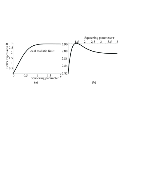
Figure 1: The Bell expression $B$ for the NOPA state as a function of the squeezing parameter $r$ for different ranges of $r$. The NOPA state is mapped onto a state of two entangled qutrits for which the Bell inequality for qutrits $B\!>\!2$ is analyzed. In the interval $[0,0.5]$ of $r$ there is no violation (a). For $r\!>\!0.5$ the amount of violation of the Bell inequality increases with an increase of $r$, until it reaches the maximal value at $r=1.4998$ ($B=2.9011$). With further increase of $r$, $B$ begins to decrease reaching asymptotically the value of $2.87293$ (b).

In this paper we use the representation in terms of the generators of the SU(n) algebra to establish the correspondence between CV and discrete systems. The particular representation is of no importance; other representations could also be possible. However, the central point should always be the use of the transition-projector operators as given in Eq. (10).

In conclusion, we find a correspondence between the CV quantum systems and discrete quantum systems of arbitrary dimension. This enables to apply all results of the physics of quantum information processing known for discrete systems also to CV systems.

This work is supported by the Austrian FWF project F1506, and by the QIPC program of the EU. MSK acknowledges the financial support by the UK Engineering and Physical Sciences Research Council through GR/R33304. We thank Jinhyoung Lee and Wonmin Son for helpful comments and discussions.

References

- (1)
- (2) M. A. Nielsen and I. L. Chuang, Quantum Computation and Quantum Information, (Cambridge University Press, 2000).
- (3) L. Vaidman, Phys. Rev. A 49, 1473 (1994); S. L. Braunstein and H. J. Kimble, Phys. Rev. Lett. 80, 869 (1998); A. Furusawa et al., Science 282, 706 (1998).
- (4) R.E.S. Polkinghorne and T.C. Ralph, Phys. Rev. Lett. 83, 2095 (1999).
- (5) L.-M. Duan et al., Phys. Rev. Lett. 84, 4002 (2000).
- (6) S. Lloyd and S. L. Braunstein, Phys. Rev. Lett. 82, 1784 (1999).
- (7) S. L. Braunstein, Phys. Rev. Lett. 80, 4084 (1998); S. Lloyd and J.-J. E. Slotine, ibid. 80, 4088 (1998); S. L. Braunstein, Nature (London) 394, 47 (1998).
- (8) S. L. Braunstein and H. J. Kimble, Phys. Rev. A 61, 042302 (2000).
- (9) N. J. Cerf, A. Ipe, and X. Rottenberg, Phys. Rev. Lett. 85, 1754 (2000).
- (10) L.-M. Duan et al. Phys. Rev. Lett. 84, 2722 (2000); R. Simon, Phys. Rev. Lett. 84, 2726 (2000).
- (11) K. Banaszek and K. Wódkiewicz, Phys. Rev. A 58, 4345 (1998); M. S. Kim and J. Lee, Phys. Rev. A 61, 042102 (2000).
- (12) Z.-B. Chen et al, Phys. Rev. Lett. 88, 040406 (2002).
- (13) L. Mišta, Jr., R. Filip, J. Fiurášek, Phys. Rev. A 65, 062315 (2002).
- (14) J. F. Clauser et al, Phys. Rev. Lett. 23, 880 (1969).
- (15) A. Einstein, B. Podolsky, and N. Rosen, Phys. Rev. 47, 777 (1935).
- (16) D. Kaszlikowski et al, Phys. Rev. Lett. 85, 4418 (2000)
- (17) D. Collins et al, Phys. Rev. Lett. 88, 040404, 2002.
- (18) N. J. Cerf et al, Phys. Rev. Lett. 88, 127902 (2002); D. Bruß and C. Macchiavello, ibid, 127901.
- (19) A. Ambainis, in Proceedings of STOC 2001, 134-142.
- (20) M. Fitzi, N. Gisin, and U. Maurer, Phys. Rev. Lett. 87, 217901 (2001).
- (21) Č. Brukner, M. Żukowski, and A. Zeilinger, Phys. Rev. Lett. 89, 197901 (2002).
- (22) F. T Hioe, and J. H. Eberly, Phys. Rev. Lett. 47, 838 (1981).
- (23) J. Schlienz, and G. Mahler, Phys. Rev A, 52, 4396 (1995).
- (24) K. Banaszek and K. Wódkiewicz, Acta Phys. Slov. 49, 491 (1999).
- (25) M. Żukowski, A. Zeilinger, M. A. Horne, Phys. Rev. A 55,2564 (1997).
- (26) L.-B. Fu, J.-L. Chen and X.G. Zhao, e-print quant-ph/0208150.
- (27) A. Acin, T. Durt, N. Gisin, and J. I. Latorre, e-print quant-ph/0111143.