Beable trajectories for revealing quantum control mechanisms

Abstract

The dynamics induced while controlling quantum systems by optimally shaped laser pulses have often been difficult to understand in detail. A method is presented for quantifying the importance of specific sequences of quantum transitions involved in the control process. The method is based on a “beable” formulation of quantum mechanics due to John Bell that rigorously maps the quantum evolution onto an ensemble of stochastic trajectories over a classical state space. Detailed mechanism identification is illustrated with a model 7-level system. A general procedure is presented to extract mechanism information directly from closed-loop control experiments. Application to simulated experimental data for the model system proves robust with up to 25% noise.

1 Introduction

Advances in pulse shaping for ultrafast lasers, fast detection techniques, and their integration via closed-loop algorithms have made it possible to control the dynamics of a variety of quantum systems in the laboratory. Excitation may be either in the strong or weak field regime, with the goal of obtaining some desired final state. Success in achieving that goal is gauged by a detected signal (e.g., the mass spectrum in the case of selective molecular fragmentation), and this information is fed back into a learning algorithm [1], which alters the laser pulse shape for the next round of experiments. High duty cycles of $\sim 0.1$ seconds or less per control experiment make it possible to iterate this process many times and perform efficient experimental searches over a control parameter space defining the laser pulse shape.

As an example of this process, experiments have employed closed-loop methods for selective fragmentation and ionization of organic [2] and organometallic [3] [4] compounds, as well as for enhancing optical response in solid-state and other chemical systems [5] [6] [7] [8]. Yields of targeted species are typically enhanced considerably over those obtained by non-optimized methods. It is found that the optimal pulse shapes achieving these enhancements can be quite complicated, and understanding their physical significance has proven difficult. The same general observations also apply to the many optimal control design simulations carried out in recent years [9] [10] [11] [12].

The present paper will address the identification of control mechanisms in theoretical calculations as well as for direct application in the laboratory. In §2 we will first describe John Bell’s beable model for finite dimensional Hilbert spaces, in order to obtain a precise (but non-unique) definition of “mechanism” for quantum systems in terms of trajectories over their associated classical state spaces. For instance, in molecular systems a trajectory would take the form of a sequence of transitions that starts with a given initial molecular configuration and switches to another configuration at a distinct time $t_{1}$, and then to another at $t_{2}$, etc.—to be contrasted with a continuously changing superposition of many such configurations.

The means to numerically implement this mechanism concept is presented in §3. An application to the problem of population transfer for a model 7-level system is given in §4, which illustrates the usefulness of mechanism information in understanding control processes. We then show how the beable approach leads to the laboratory working relations (17) and (18), which make it possible to identify some basic aspects of control mechanisms directly from experimental data. We illustrate this process in §6 on simulated experimental data for the model 7-level system. The overall laboratory algorithm for extracting control mechanism information is condensed into a general-purpose procedure in §7.

2 Beables and quantum theory

Consider a control problem posed in terms of the quantum evolution

$$\mathrm{i}\hbar\frac{d}{dt}|\psi(t)\rangle=H(t)|\psi(t)\rangle$$ (1)

over a finite dimensional Hilbert space with basis $|n\rangle$ where $n=0,1,2,\ldots$. Here $H(t)=H_{0}-\mu E(t)$ incorporates the effect of the control field $E(t)$, and we can explicitly follow the evolution of $|\psi\rangle$ into a desired final state $|\psi(t_{\mathrm{f}})\rangle$.

This paper is concerned with the question: what is the importance of a given sequence $n_{1}\rightarrow n_{2}\rightarrow\cdots$ of actual transitions—or, more specifically, of a given trajectory defined as a continuous function $n(t)$ of time—in achieving the desired final state $|\psi(t_{\mathrm{f}})\rangle$? In other words, it is clear that the system is being driven into a desired state, but can we find a physical picture of how this is being accomplished?

A conventional answer to the question raised above, essentially that given by Bohr on first seeing Feynman’s path integral, is to reject the question as ill-posed because quantum mechanics is said to forbid consideration of precisely defined trajectories over the classical state space $\{n\}$. Nevertheless, it is well established that there exist dynamical models generating an ensemble of trajectories $n(t)$ whose statistical properties exactly match those associated with $|\psi(t)\rangle$ at each $t$. In the case of a continuous state space, the first such model was that of de Broglie, later rediscovered and completed by Bohm [15]. They reintroduce classical-like particle trajectories into quantum theory by taking the probability current $\mathbf{J}[\psi]$ to describe a statistical ensemble of real particles. So,

$$\mathbf{v}=\frac{\mathbf{J}}{|\psi|^{2}}=\mathrm{Re}\left\{-\mathrm{i}\frac{\hbar}{m}\frac{\nabla\psi(\mathbf{x},t)}{\psi(\mathbf{x},t)}\right\}$$ (2)

gives the velocity of a particle with mass $m$ and position $\mathbf{x}$ at time $t$, in de Broglie-Bohm (dBB) theory. The physical particle is taken to exist independently of, but also to have its motion determined by, the wavefunction $\psi$. The time evolution of $\psi$ itself is just given by the Schrodinger equation.

Bohm developed a full account of how ensembles of such classical-like particles could reproduce the predictions of quantum mechanics. A basic issue is to compare $\psi(\mathbf{x},t)$ with the statistical distribution $P(\mathbf{x},t)$ describing an ensemble of particles evolving by (2). One can show that if the initial distribution of particles satisfies $P(\mathbf{x},0)=|\psi(\mathbf{x},0)|^{2}$, then $P(\mathbf{x},t)=|\psi(\mathbf{x},t)|^{2}$ will hold for all $t>0$. That is, if the ensemble is initially in the “quantum equilibrium” distribution given by $|\psi(\mathbf{x},0)|^{2}$, the dynamics—(2) for the particles, and the Schrodinger equation for $\psi$—will preserve this equilibrium, consistent with the predictions of standard quantum theory. The result is easily generalized to arbitrary interacting $N$-particle systems by taking $\mathbf{x}$ as a point in the $3N$ dimensional configuration space.

In dBB theory the position representation has a special status. While one may still regard $\psi$ as a basis-independent object, the particle dynamics is given by (2) specifically in terms of $\langle\mathbf{x}|\psi\rangle$ rather than $\langle\mathbf{p}|\psi\rangle$ or some other representation. But, it is easy to formulate analogs of dBB theory in different bases. For instance, one might choose the momentum values $\mathbf{p}$ as the beables of the theory, and the dBB trajectories $\mathbf{x}(t)$ would be replaced by momentum space trajectories $\mathbf{p}(t)$.

In the context of a finite dimensional Hilbert space with basis $|n\rangle$, the beables can be taken as the sites $n$ of the classical state space $\{n\}$ analogous to $\{\mathbf{x}\}$ or $\{\mathbf{p}\}$. Some law analogous to (2) must be given to generate beable trajectories $n(t)$ over the state space. Such trajectories would provide a physical picture of the quantum transitions induced by a control field $E(t)$.

In one such theory due to John Bell [16], trajectories arise from beables stochastically jumping between sites connected by non-zero Hamiltonian matrix elements. To define this Broglie-Bohm-Bell (BBB) theory, the probability for a beable to jump from site $m$ to a distinct site $n$, sometime in the interval $(t,t+\epsilon)$, is taken as

$$T_{nm}(t)\epsilon=\left\{\begin{array}[]{ll}2\,\mathrm{Re}\{z_{nm}(t)\}\epsilon&\mbox{if Re$\{z_{nm}(t)\}>0$}\\ 0&\mbox{if Re$\{z_{nm}(t)\}\leq 0$}\end{array}\right.$$ (3)

where

$$z_{nm}(t)=-\frac{\mathrm{i}}{\hbar}H_{nm}\frac{\psi_{n}(t)^{\ast}}{\psi_{m}(t)^{\ast}}$$ (4)

and $\psi_{n}=\langle n|\psi\rangle$, etc. To ensure normalization, the probability for a beable to stay at $m$ is thus given by $1-\sum_{n}^{\prime}T_{nm}(t)\epsilon$, where the primed sum excludes the diagonal term $n=m$. From (4), we find

$$\mathrm{Re}\{z_{nm}\}=-\mathrm{Re}\{z_{mn}\}\frac{|\psi_{n}|^{2}}{|\psi_{m}|^{2}}$$ (5)

which implies through (3) that either $T_{nm}(t)=0$ or $T_{mn}(t)=0$ at any particular time $t$. Together with (1) this gives

$$\frac{d}{dt}|\psi_{n}|^{2}=\sum_{m}2\,\mbox{Re}\{z_{nm}|\psi_{m}|^{2}\}=\sum_{m}(T_{nm}|\psi_{m}|^{2}-T_{mn}|\psi_{n}|^{2})$$ (6)

as a type of master equation. Note that the $T_{nm}$ term contributes when Re$\{z_{nm}\}>0$, and the $T_{mn}$ term contributes when Re$\{z_{nm}\}<0$.

Now consider the probability distribution $P_{n}(t)$ of beables in state space generated by the jump rule (3). Accounting for the influx and outflux of beables at site $n$, we see $P_{n}(t)$ satisfies

$$\frac{d}{dt}P_{n}=\sum_{m}(T_{nm}P_{m}-T_{mn}P_{n})$$ (7)

which is formally identical to (6). Thus, provided $P_{n}(0)=|\psi_{n}(0)|^{2}$, we are guaranteed $P_{n}(t)=|\psi_{n}(t)|^{2}$ for all $t>0$, which expresses the equivalence of BBB theory and ordinary quantum mechanics in terms of statistical predictions.

The answer to the initial question regarding the importance of a given trajectory in achieving the desired state $|\psi(t_{\mathrm{f}})\rangle$ is now very simple. The importance may be taken as just the probability of realizing that trajectory with the jump rule (3). We can express the final state population in terms of these path probabilities via the integral (path sum) version of (7):

$$P_{n_{\mathrm{f}}}(t_{\mathrm{f}}) = \sum_{\mathcal{P}}P_{n_{0}}(0)\,\mathrm{Prob}(\mathcal{P})$$ (8)

$$\mathrm{Prob}(\mathcal{P}) = \prod_{p\in J}\epsilon T_{n_{p+1}n_{p}}\prod_{p\notin J}\left(1-\epsilon{\textstyle\sum_{n}^{\prime}}T_{nn_{p}}\right)$$

where $\mathrm{Prob}(\mathcal{P})$ is the probability of realizing the path $\mathcal{P}=(n_{0},n_{1},\ldots)$ under (3), and $n_{p}$ gives the beable configuration at $t=p\epsilon$. The first sum is taken over all such paths ending on $n_{\mathrm{f}}$ at $t=t_{\mathrm{f}}$, and $J[\mathcal{P}]=\{p\;|\;n_{p+1}\neq n_{p}\}$ defines the jump set.

The above argument for the equivalence of BBB theory and ordinary quantum mechanics ensures that the path probabilities $\mathrm{Prob}(\mathcal{P})$ are consistent with the quantum distribution $|\psi_{n}(t)|^{2}$ governing observables. But, it should be noted that BBB theory is not unique in this regard. The rule (3) may be altered in non-trivial ways while preserving the master equation (6) [18]. The definition (3) might even be changed in ways that do not preserve (6), if one is willing to relinquish a strict probability interpretation for the trajectories [13].

In general, there are many different ways to assign probabilities to trajectories that all result in the same time-dependent occupation probabilities $P_{n}(t)$. The predictions of quantum mechanics, therefore, cannot select a single assignment. This non-uniqueness at the root of quantum mechanism identification can be dealt with only by reference to the simplicity and explanatory power of a given mechanism definition. Below we adopt the definition (3).

3 Simulating beables in quantum control

An ultimate goal is to obtain dynamical mechanism information directly from experimental data associated with the closed-loop control field optimization, without pre-existing knowledge of the system Hamiltonian or wavefunction. Methods employing BBB theory for this purpose are presented in §5, but first we shall study control mechanisms for a model system whose Hilbert space and quantum evolution are given explicitly in numerical simulations.

Consider a quantum-optical system with level energies $\hbar\omega_{n}$ and dipole moments $\mu_{nm}$. Applying an external laser field $E(t)$, the Hamiltonian in the interaction picture [17] is

$$H_{I}=E(t)\sum_{n\,m}\mu_{nm}\mathrm{e}^{\mathrm{i}\omega_{nm}t}|n\rangle\langle m|$$ (9)

where $\omega_{nm}\equiv\omega_{n}-\omega_{m}$. We will drop the subscript $I$ from now on. $E(t)$ is assumed to be given by an independent optimization algorithm designed to, for example, maximally transfer population from $|n_{\mathrm{i}}\rangle$ to $|n_{\mathrm{f}}\rangle$.

A simple second-order Schrodinger propagator was used to solve (1) in the interaction picture, relying on a factorization of the evolution operator as

$$\mathcal{T}\left\{\mathrm{e}^{-\frac{\mathrm{i}}{\hbar}\int_{0}^{t}H(s)ds}\right\}=\prod_{p=0}^{N-1}\mathcal{T}\left\{\mathrm{e}^{-\frac{\mathrm{i}}{\hbar}\int_{t_{p}}^{t_{p+1}}H(s)ds}\right\}$$ (10)

where $t_{p}=p\epsilon\equiv pt_{\mathrm{f}}/N$ and $\mathcal{T}$ is the time-ordering symbol. Choosing a time step $\epsilon\ll\hbar/\mu E$, we can approximate (10) by dropping the $\mathcal{T}$ operations on the right hand side and computing the integrals directly. In doing this an error is accrued per time step given by the Baker-Hausdorf identity $\mathrm{e}^{A+B}=\mathrm{e}^{A}\mathrm{e}^{B}\mathrm{e}^{-\frac{1}{2}[A,B]+\cdots}$ as

$$\frac{1}{\hbar^{2}}\int_{t_{p}}^{t_{p+1}}\int_{t_{p}}^{t_{p+1}}[H(r),H(s)]\,dr\,ds\;\sim\;\left(\frac{\mu E}{\hbar}\right)^{2}\epsilon^{3}\omega\,.$$ (11)

The right hand estimate is obtained by expanding $H(r)$ to first order about $r=s$ and noticing that the $E^{\prime}(s)$ term in $H^{\prime}(s)$ commutes with $H(s)$. The error (11) would generally dominate third order terms like $(\mu E\epsilon/\hbar)^{3}$.

If the control field is given as $E(t)=\mathrm{Re}\{\sum_{i}\alpha_{i}E_{i}(t)\}$, where

$$E_{i}(t)=A(t)\mathrm{e}^{\mathrm{i}(\phi(t)+\omega_{i}^{\mathrm{c}}t)}$$

with $A(t)$ and $\phi(t)$ possibly adiabatic, we can evaluate $\int H(s)ds$ by writing

$$\int_{t_{p}}^{t_{p+1}}\mu E_{i}(s)\mathrm{e}^{\mathrm{i}\omega s}ds\;\approx\;\frac{\mu A(t_{p})\mathrm{e}^{\mathrm{i}\phi(t_{p})}}{\mathrm{i}(\omega+\omega_{i}^{\mathrm{c}})}\left(\mathrm{e}^{\mathrm{i}(\omega+\omega_{i}^{\mathrm{c}})t_{p+1}}-\mathrm{e}^{\mathrm{i}(\omega+\omega_{i}^{\mathrm{c}})t_{p}}\right)\;.$$ (12)

(Simply writing $\int H(s)ds\approx\epsilon H(t_{p})$ is not appropriate because we do not want to exclude weak field excitation, i.e. $\mu E\ll\hbar\omega$, so that $\omega\epsilon\sim 1$ may hold.) Thus in the adiabatic case $|\psi(t)\rangle$ can be propagated in steps determined by $A(t)$ and $\phi(t)$ rather than the phase factors $\mathrm{e}^{\mathrm{i}\omega t}$.

Consider the evolution of beable trajectories according to (3), which appears to require a time step small enough that each part of $H$, including the $\mathrm{e}^{\mathrm{i}\omega t}$ terms, not vary much over the step. Nevertheless, the total probability of jumping from $m$ to $n$ over $(t_{p},t_{p+1})$ is given by the integral $\int T_{nm}(s)ds$ over that range with $\sim(\mu E\epsilon/\hbar)^{2}$ corrections. Thus we can take an effective jump probability for the interval $(t_{p},t_{p+1})$ as given by (3) with

$$z_{nm}(t_{p})\;\approx\;-\frac{\psi_{n}(t_{p})^{\ast}}{\psi_{m}(t_{p})^{\ast}}\frac{\mathrm{i}}{\hbar\epsilon}\int_{t_{p}}^{t_{p+1}}H_{nm}(s)ds$$ (13)

evaluated using (12). If $\omega\epsilon\ll 1$ does not hold, care must be taken to extend the integration in (13) only over $t\in(t_{p},t_{p+1})$ for which $\mathrm{Re}\{z_{nm}(t)\}>0$, leading to additional boundary terms in the phase difference part of (12). Moving the $\psi^{\ast}$ ratio outside the integral in (13) produces an error per time step of order

$$\frac{\epsilon^{2}H}{\hbar}\frac{\partial\psi}{\partial t}\;\sim\;\left(\frac{\mu E\epsilon}{\hbar}\right)^{2}$$

which is again comparable to (11). Therefore beable trajectories may be propagated in steps determined by $A(t)$ and $\phi(t)$, i.e. in sink with the Schrodinger propagator.

4 A model 7-level system: mechanism analysis of an optimal control design

The beable trajectory methodology for identification of control mechanisms will be illustrated with a 7-level system where $\omega_{n}$ and $\mu_{nm}$ are given in Fig. 1. The (non-adiabatic) control field $E(t)$ shown in Fig. 2 is obtained from a steepest descents algorithm over the space of field histories [14]. It is optimized to transfer population from the ground state $|0\rangle$ to the highest excited state $|6\rangle$. By $t=100$ fs, the transfer is found to be completed with approximately 97% efficiency (see Fig. 3).

Together with the second-order Schrodinger propagator, using time step $\epsilon=.025$ fs, an ensemble of $N_{\mathrm{traj}}=10^{5}$ beable trajectories is evolved, all starting in the ground state $n=0$ at $t=0$. At each time step, a given beable at site $m$ is randomly made either to jump to a neighboring site $n\neq m$ according to the probabilities $T_{nm}\epsilon$ given by (3) with (13), or else stay at $m$. Four sample trajectories are shown in Fig. 4. As a check, one can count the number of beables residing on each site $n$ at time $t$ to estimate the occupation probabilities $P_{n}(t)$ and verify that they match the quantum prescriptions $|\psi_{n}(t)|^{2}$. The finite-ensemble deviations are observed to be consistent with a $(N_{\mathrm{traj}})^{-1/2}$ convergence law.

About 60% of the trajectories generated are found to involve four jumps, and of these the trajectories passing through sites $n=2,5$ are noticeably more probable than those passing through $n=1,4$. 6-jump trajectories comprise about 30% of the ensemble. And it becomes increasingly less likely to find trajectories with more and more jumps. The largest number of jumps observed in a single trajectory was 14. Three such trajectories occurred out of the ensemble total $10^{5}$.

A natural expectation is that the optimal field $E(t)$ would concentrate on the higher probability trajectories and not waste much effort on guiding highly improbable trajectories, such as the 14-jumpers, to the target state $n=6$, as the latter have essentially no impact on the control objective (final population of the target state). Interestingly, though, the vast majority of even the lowest probability trajectories are still guided to $n=6$. Apparently, the optimal field is able to coordinate its effect on low probability trajectories with that on other trajectories at no real detriment to the latter. We shall come back to this point later.

One way to conveniently categorize the large set of trajectories, each expressible as a sequence of time-labeled jumps $(t_{1},n_{1})\rightarrow(t_{2},n_{2})\rightarrow\cdots$, is to drop the time labels, leaving only the “pathway” $n_{1}\rightarrow n_{2}\rightarrow\cdots$. The importance of a given pathway is then computed as the frequency of trajectories associated with that pathway. Table 1 lists some important and/or interesting pathways and their probabilities.

Fig. 5 shows some typical trajectories associated with the first and fifth pathways listed in Table 1—involving 4 and 6 jumps respectively. $E(t)$ guides the 4-jumpers upward in energy, and they begin to arrive at $n=6$ around $t=80$ fs, early enough that stragglers can catch up but too late for the over-achievers of the group to head off elsewhere. This corresponds to the onset of heavy growth for $|\psi_{6}(t)|^{2}$ around $t=80$ fs (see Fig. 3). The 6-jumpers first reach $n=6$ around $t=50$ fs, but almost all fall back to $n=5$ by $t=80$ fs, reuniting with the 4-jumpers just as they begin to jump up to $n=6$. These 6-jumpers, along with other high-order contributions, thus explain the small surge in $|\psi_{6}(t)|^{2}$ between 50 and 80 fs. Another much smaller surge around $t=30$ fs and one still smaller around $t=20$ fs (see inset of Fig. 3) are attributable to 8-th and higher order trajectories “ringing” back and forth on $5\leftrightarrow 6$.

For $t\in(70\mbox{ fs},80\mbox{ fs})$, many of the 6-jumpers are at $n=6$ and need to be de-excited on the $6\rightarrow 5$ transition before they can jump back up to $n=6$. Simultaneously, many of the 4-jumpers are at $n=5$ and should not be prematurely excited on $5\rightarrow 6$, lest they not remain at $n=6$ through $t=100$ fs. The optimal field thus faces a conundrum: how to stimulate the $2\leftrightarrow 6$ transition preferentially for the 6-jumpers (in $n=6$) over the 4-jumpers (in $n=5$). The means by which this feat is accomplished may be understood by reference to the jump rule (3). $E(t)$ induces jumps through the explicit $H_{nm}(t)$ factor but also through the $\psi^{\ast}$ quotient, which depends on $E(t)$ through $(\ref{schrod})$. In particular, (5) implies that at any one time $t$ jumps on this transition must be either all upward or all downward. The active direction is switched back and forth according to the sign of $\mathrm{Re}\{z_{65}(t)\}$.

Fig. 6 plots $|E(t)|$ and $\mathrm{Re}\{z_{65}(t)\}$, which controls the upward jump rate $T_{65}(t)$. For $t\in(70\mbox{ fs},80\mbox{ fs})$ one sees that when $|E(t)|$ is large, most often $\mathrm{Re}\{z_{65}(t)\}$ dips below zero, disallowing any upward jumps. The correlation coefficient between $|E(t)|$ and $\mathrm{Re}\{z_{65}(t)\}$ in this range is $-0.4955$. On the other hand, the correlation between $|E(t)|$ and $\mathrm{Re}\{z_{56}(t)\}$, which controls downward jumping, is $+0.4475$ over the same range.

Looking at the trajectories in more detail, one notices a distinct bunching of jumps. Beables tend to jump together in narrow time bands, or else to abstain in unison from jumping. This behavior can be gauged by calculating the two-time jump-jump correlation function:

$$J_{\Omega}^{(2)}(\tau)\equiv\frac{1}{N}\sum_{p=0}^{N-1}J_{\Omega}(t_{p})J_{\Omega}(t_{p}+\tau)$$

where $J_{\Omega}(t)$ is the number of jumps of type $\Omega$ occurring in $(t,t+\epsilon)$, and $\Omega$ is a subset of the entire ensemble of trajectories. For instance, the two-time function with $\Omega$ taken as the set of jumps on the $5\rightarrow 6$ transition is plotted in Fig. 7. The fs time-scale oscillations correspond to the level splittings $\omega_{nm}$ and the dominant frequency components of $E(t)$. Enhanced correlations around $\tau=0$ correspond to the jump bunching noticeable in the trajectories. Two side-bands around $\tau=\pm 40$ fs are associated with 6-jump and higher order trajectories that go up, down, and up again on $5\leftrightarrow 6$ over the approximate time window $(50\mbox{ fs},90\mbox{ fs})$. This conclusion can be verified by computing two-time functions with $\Omega$ specialized to particular pathways. Other much smaller features for $|\tau|>60$ fs (see inset of Fig. 7) are attributable to higher order trajectories ringing on $5\leftrightarrow 6$.

In general, the fs oscillations characteristic of these two-time functions show that $E(t)$ works in an essentially discrete way, turning on the flow of beables over a given transition and then turning it off with a duty cycle of $\approx 2$ fs. The associated bandwidth of $\approx 0.5\mbox{ fs}^{-1}$ is small enough to discriminate between all non-degenerate $\omega_{nm}$ except between $\omega_{35}(=\omega_{34})$ and $\omega_{56}(=\omega_{46})$, which differ by only $0.12\mbox{ fs}^{-1}$. This circumstance leaves effectively three distinguishable transitions. With a total time of 100 fs, the control field $E(t)$ can potentially enact roughly $150$ separate flow operations. The fact that trajectories with pathway probability $\ll 1$% are still almost always guided successfully to $n=6$ suggests that these $\sim 150$ operations are more than necessary to obtain the 97% success rate achieved by the optimal control algorithm in this simulation. It appears that the algorithm actively sweeps these aberrant trajectories back into the mainstream so as to maximize even their minute contribution to the control objective.

5 Control mechanism identification in the laboratory

Using these beable trajectory methods to extract mechanism information directly from closed-loop data is complicated by the fact that we cannot assume knowledge of a time-dependent wavefunction, Hamiltonian, or possibly even the energy level structure of the system. Frequently in the laboratory, the only available information consists of final state population measurements and knowledge of the control field $E(t)$.

The following analysis aims to show how a limited statistical characterization of beable trajectories may be generated from laboratory data associated with a given optimal control field. In particular, we will show how to extract $j_{\mathrm{min}}$, the minimum number of jumps necessary to reach the final state $n_{\mathrm{f}}$ from the initial state $n_{\mathrm{i}}$; also $\langle j_{\mathcal{P}}\rangle$, the average number of such jumps over an ensemble of beable trajectories; and possibly higher moments $\langle(j_{\mathcal{P}})^{k}\rangle$ as well. After a general formulation of this analysis is presented, it will be applied to simulated experimental data in the case of the model 7-level system considered above.

We propose to obtain mechanism information by examining the effect on the final state population $|\psi_{n_{\mathrm{f}}}|^{2}$ of variations in the control field away from optimality. Consider the simplest such scheme, wherein the amplitude of the control field is modulated by a constant $\mathcal{M}$ independent of time:

$$E(t)\rightarrow\tilde{E}(t)=\mathcal{M}E(t)$$

giving rise to a new time-dependent solution $|\tilde{\psi}(t)\rangle$—in particular, a new final state population $|\tilde{\psi}_{n_{\mathrm{f}}}(t_{\mathrm{f}})|^{2}$ and new path probabilities P$\widetilde{\mathrm{rob}}(\mathcal{P})$. These quantities are obtained by taking $T_{nm}\rightarrow\tilde{T}_{nm}$ in (8), which is to say using $\tilde{E}(t)$ and $\tilde{\psi}_{n}(t)$ in the jump rule (3).

To express P$\widetilde{\mathrm{rob}}(\mathcal{P})$ in terms of Prob$(\mathcal{P})$, we can write

$$\prod_{p\in J}\tilde{T}_{n_{p+1}n_{p}} = \mathcal{M}^{j_{\mathcal{P}}}\prod_{p\in J}T_{n_{p+1}n_{p}}\prod_{p\in J}\frac{\cos\tilde{\phi}_{p}}{\cos\phi_{p}}\;\times$$ (14)

$$\;\;\prod_{p\in J}\frac{|\tilde{\psi}_{n_{p+1}}(t_{p})|}{|\tilde{\psi}_{n_{p}}(t_{p})|}\left(\prod_{p\in J}\frac{|\psi_{n_{p+1}}(t_{p})|}{|\psi_{n_{p}}(t_{p})|}\right)^{-1}$$

where $j_{\mathcal{P}}$ is the number of jumps in $\mathcal{P}$ and

$$\tilde{\phi}_{p}\;\equiv\;\arg\left(-\mathrm{i}H_{n_{p+1}n_{p}}\frac{\tilde{\psi}_{n_{p+1}}(t_{p})}{\tilde{\psi}_{n_{p}}(t_{p})}\right)\,.$$

To simplify (14), note that if $j_{\mathcal{P}}$ were very large, then successive terms in each of the last two products would tend to cancel, leaving only endpoint contributions. Making the reasonable approximation that they do completely cancel yields

$$\prod_{p\in J}\tilde{T}_{n_{p+1}n_{p}}\;\approx\;\mathcal{M}^{j_{\mathcal{P}}}\,\frac{|\tilde{\psi}_{n_{\mathrm{f}}}(t_{\mathrm{f}})|}{|\psi_{n_{\mathrm{f}}}(t_{\mathrm{f}})|}\,\prod_{p\in J}T_{n_{p+1}n_{p}}\prod_{p\in J}\frac{\cos\tilde{\phi}_{p}}{\cos\phi_{p}}\,.$$ (15)

Further, we can make the expansion

$$-\log\prod_{p\in J}\frac{\cos\tilde{\phi}_{p}}{\cos\phi_{p}}\;=\;a_{\mathcal{P}}^{(1)}(\mathcal{M}-1)+a_{\mathcal{P}}^{(2)}(\mathcal{M}-1)^{2}+\cdots$$

about $\mathcal{M}=1$, where the $a_{\mathcal{P}}^{(i)}$ depend on the path $\mathcal{P}$ but not on $\mathcal{M}$. And similarly:

$$-\log\prod_{p\notin J}\left(1-\epsilon{\textstyle\sum_{n}^{\prime}}\tilde{T}_{nn_{p}}\right) \approx \epsilon{\textstyle\sum_{p\notin J}}{\textstyle\sum_{n}^{\prime}}\tilde{T}_{nn_{p}}$$

$$= \epsilon{\textstyle\sum_{p\notin J}}{\textstyle\sum_{n}^{\prime}}T_{nn_{p}}+b_{\mathcal{P}}^{(1)}(\mathcal{M}-1)+\cdots$$

Combining these expansions gives a relationship between the path probabilities P$\widetilde{\mathrm{rob}}(\mathcal{P})$ in the modulated case to those, Prob$(\mathcal{P})$, in the unmodulated case, which are the ones containing mechanism information regarding the actual optimal control field $E(t)$. We can thus write the final population as

$$|\tilde{\psi}_{n_{\mathrm{f}}}(t_{\mathrm{f}})|^{2} = \sum_{\mathcal{P}}|\psi_{n_{0}}(0)|^{2}\,\mbox{P$\widetilde{\mathrm{rob}}(\mathcal{P})$}$$

$$\approx \frac{|\tilde{\psi}_{n_{\mathrm{f}}}(t_{\mathrm{f}})|}{|\psi_{n_{\mathrm{f}}}(t_{\mathrm{f}})|}\sum_{\mathcal{P}}|\psi_{n_{0}}(0)|^{2}\mathcal{M}^{j_{\mathcal{P}}}\mathrm{e}^{-a_{\mathcal{P}}(\mathcal{M}-1)}\,\mathrm{Prob}(\mathcal{P})$$

where $a_{\mathcal{P}}\equiv a_{\mathcal{P}}^{(1)}+b_{\mathcal{P}}^{(1)}$, and higher order terms in the expansion have been dropped. (This approximation is not as crude as it might seem, since for small $\mathcal{M}$ away from 1, the behavior of $|\tilde{\psi}_{n_{\mathrm{f}}}(t_{\mathrm{f}})|^{2}$ is dominated by the $\mathcal{M}^{j_{\mathcal{P}}}$ factor.) Cancelling one power of $|\tilde{\psi}_{n_{\mathrm{f}}}(t_{\mathrm{f}})|$, and recalling that the sum is taken only over paths ending on $n=n_{\mathrm{f}}$ so that $|\psi_{n_{\mathrm{f}}}(t_{\mathrm{f}})|^{2}=\sum_{\mathcal{P}}\mathrm{Prob}(\mathcal{P})$, we have

$$|\tilde{\psi}_{n_{\mathrm{f}}}(t_{\mathrm{f}})|\;\approx\;|\psi_{n_{\mathrm{f}}}(t_{\mathrm{f}})|\left\langle\mathcal{M}^{j_{\mathcal{P}}}\mathrm{e}^{-a_{\mathcal{P}}(\mathcal{M}-1)}\right\rangle$$ (16)

where $\langle\cdots\rangle$ denotes an average over the trajectory ensemble generated by the (unmodulated) optimal field $E(t)$. Beables in this ensemble are taken as initially distributed at $t=0$ according to $|\psi_{n}(0)|^{2}$, and only trajectories that successfully reach $n=n_{\mathrm{f}}$ at $t=t_{\mathrm{f}}$ are counted.

Note that for $\mathcal{M}$ close enough to 0, the minimum value $j_{\mathrm{min}}$ taken on by $j_{\mathcal{P}}$ will dominate the expectation value in (16), and

$$\log|\tilde{\psi}_{n_{\mathrm{f}}}(t_{\mathrm{f}})|=j_{\mathrm{min}}\log\mathcal{M}+\mathrm{O}(1)$$ (17)

gives the dominant behavior independent of $a_{\mathcal{P}}$. If we suppose that $a_{\mathcal{P}}$, where it is relevant, depends primarily on the endpoints of $\mathcal{P}$, which are fixed, and only weakly on the rest of the path, then $a_{\mathcal{P}}$ can be approximated by some characteristic value $a$. Putting $\mathcal{M}^{j_{\mathcal{P}}}=\mathrm{e}^{j_{\mathcal{P}}\log\mathcal{M}}$ in (16) and expanding in powers of $\log\mathcal{M}$ now gives

$$|\tilde{\psi}_{n_{\mathrm{f}}}(t_{\mathrm{f}})|\;\approx\;|\psi_{n_{\mathrm{f}}}(t_{\mathrm{f}})|\,\mathrm{e}^{-a(\mathcal{M}-1)}\sum_{k=0}^{\infty}\frac{\langle(j_{\mathcal{P}})^{k}\rangle}{k!}(\log\mathcal{M})^{k}$$ (18)

for the final state population under a modulated field, expressed in terms of the desired statistical properties of the trajectory ensemble under the optimal field itself. Here, $a$ enters as an additional parameter that must be extracted from the data. Equations (17) and (18) form the working relations to extract mechanism information from laboratory data.

6 Simulated experiments on a 7-level system

In order to extract quantities like $\langle j_{\mathcal{P}}\rangle$ using the results (17) and (18) data must be generated for the final state population $|\tilde{\psi}_{n_{\mathrm{f}}}(t_{\mathrm{f}})|^{2}$ at many values of the modulation factor $\mathcal{M}$ over some range $(\mathcal{M}_{\mathrm{min}},\mathcal{M}_{\mathrm{max}})\sim(0,1.5)$. The desired quantities are obtained as parameters in fitting (17) and (18) to the data as a function of $\mathcal{M}$.

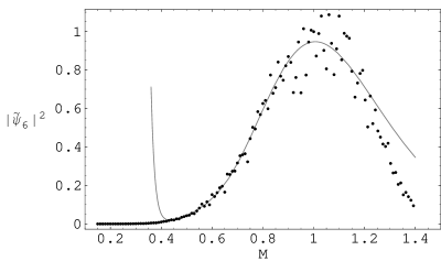
Figure 8: The best fit of (18) to the simulated $|\tilde{\psi}_{n_{\mathrm{f}}}(t_{\mathrm{f}})|^{2}$ data (10% noise) as a function of $\mathcal{M}$; it occurs over the fitting range $\mathcal{M}\in(.44,.92)$.

One set of simulated data for the above 7-level system is shown in Fig. 8; the sampling increment is $\Delta M=.01$. Noise has been introduced by multiplying the exact $|\tilde{\psi}_{n_{\mathrm{f}}}(t_{\mathrm{f}})|^{2}$ values by an independent Gaussian-distributed random number for each value of $\mathcal{M}$, where the distribution is chosen to have mean 1, and various standard deviations $\sigma$ have been sampled.

We can determine $j_{\mathrm{min}}$ from the data using (17), which implies

$$j_{\mathrm{min}}=\lim_{\mathcal{M}\rightarrow 0}\frac{d\log|\tilde{\psi}_{n_{\mathrm{f}}}(t_{\mathrm{f}})|}{d\log\mathcal{M}}\,.$$ (19)

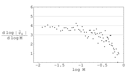
Figure 9: The derivative is calculated from simulated data with noise level $\sigma=.1$; its limiting value as $\log\mathcal{M}\rightarrow-\infty$ gives $j_{\mathrm{min}}$.

For instance, Fig. 9 plots the derivative in (19), calculated with finite differences from the $|\tilde{\psi}_{n_{\mathrm{f}}}(t_{\mathrm{f}})|^{2}$ simulated data for $\sigma=.1$, which correctly gives $j_{\mathrm{min}}=4$ as the limiting value. Determination of $j_{\mathrm{min}}$ proved robust to multiplicative Gaussian noise up to the 40% level ($\sigma=.4$).

The quantity $\langle j_{\mathcal{P}}\rangle$ is more difficult to extract, because while the sum in (18) converges to 0 as $\mathcal{M}\rightarrow 0$, the terms of the sum individually diverge and must cancel in a delicate manner. Therefore truncating the sum to an upper limit $k_{\mathrm{max}}$ becomes a very bad approximation near $\mathcal{M}=0$. This unstable behavior can be controlled by carefully setting the range $(\mathcal{M}_{\mathrm{min}},\mathcal{M}_{\mathrm{max}})$ of data to be fitted, given a choice of $k_{\mathrm{max}}$.

It is also convenient to constrain the fit by the previous determination of $j_{\mathrm{min}}=4$. We have done this by noting that if $E(t)$ is truly optimal, then $|\tilde{\psi}_{n_{\mathrm{f}}}(t_{\mathrm{f}})|$ must have a maximum at $\mathcal{M}=1$, which implies that $a=\langle j_{\mathcal{P}}\rangle$. This can be used as a weaker constraint on the auxiliary parameter $a$ by just requiring $a>j_{\mathrm{min}}=4$ in the fit without necessarily supposing that $E(t)$ is exactly optimal. We then check that $a\approx\langle j_{\mathcal{P}}\rangle$ is satisfied in the fit. Fig. 8 shows one such fit where the fitting range is $\mathcal{M}\in(.44,.92)$. One can see that the fit closely tracks the data for $\mathcal{M}$ in this range but quickly diverges from the data just below $\mathcal{M}=.44$ (and, less severely, above $\mathcal{M}=.92$) due to the sum-truncation instability mentioned previously.

In order to identify appropriate ranges in general, we have searched over all combinations such that

$$\begin{array}[]{c}\begin{array}[]{lcccr}.2&<&\mathcal{M}_{\mathrm{min}}&<&.8\\ .7&<&\mathcal{M}_{\mathrm{max}}&<&1.6\\ \end{array}\\ \mathcal{M}_{\mathrm{max}}-\mathcal{M}_{\mathrm{min}}>10\end{array}$$ (20)

Mathematica’s implementation of the Levenberg-Marquardt non-linear fitting algorithm was used on simulated data for each value of $\sigma$ between 0 and .5 with a .01 increment. The best fit at each $\sigma$ was used to determine the value of $\langle j_{\mathcal{P}}\rangle$ most consistent with the simulated data at the given noise level.

For this analysis $k_{\mathrm{max}}=4$ was chosen somewhat arbitrarily to balance computational cost and precision. In practice it is likely that the moments $\langle(j_{\mathcal{P}})^{k}\rangle$ for lower $k$ values will be most reliably extracted from the data, especially considering the laboratory noise. In the simulations it was found that $\langle j_{\mathcal{P}}\rangle$ could be reliably extracted, but higher moments were unstable and unreliable. For example, $\langle(j_{\mathcal{P}})^{2}\rangle$ was frequently found to lie slightly below the corresponding fit values for $\langle j_{\mathcal{P}}\rangle^{2}$, which is inconsistent with the interpretation of these values as statistical moments of an underlying random variable $j_{\mathcal{P}}$. Further constraints could be introduced to attempt to stabilize the extraction of higher moments, but care is needed so as not to overfit the data.

Fig. 10 shows the $\langle j_{\mathcal{P}}\rangle$ values obtained by fitting data with $\sigma=.1$ for each choice of $(\mathcal{M}_{\mathrm{min}},\mathcal{M}_{\mathrm{max}})$ and Fig. 11 shows the corresponding quality of each fit as measured by its mean squared deviations. In Fig. 10, as well as in the corresponding plots for all other values of $\sigma$ studied, two diagonal strips emerge running above a set of smaller islands. The surrounding white “sea” comprises fits that give $\langle j_{\mathcal{P}}\rangle<4$, which we know to be ruled out by the determination of $j_{\mathrm{min}}$.

A virtually identical pattern arises in the fit quality plots. The two strips and underlying islands are seen to give much better fits than the white sea. An additional connected region of good fits is found to extend across the lower-left corner of Fig. 11, nearly all of which are ruled out by $j_{\mathrm{min}}=4$. This connected region is somewhat pathological because much of it corresponds to fitting ranges that fail to capture the important behavior of $|\tilde{\psi}_{n_{\mathrm{f}}}(t_{\mathrm{f}})|^{2}$ near $\mathcal{M}=1$, and therefore can be ignored. Then the best fits for all values of $\sigma$ sampled are found to come from the cluster of islands at $\mathcal{M}_{\mathrm{max}}\approx.95$. As $\sigma$ is increased from 0 to .5, these islands flow from $\mathcal{M}_{\mathrm{min}}\approx.5$ to $\mathcal{M}_{\mathrm{min}}\approx.3$, carrying with them the best fit site. Note that the small triangular area in the lower right corner, most noticeable in Fig. 11, is a region excluded from consideration by the third constraint in (20).

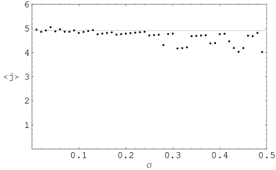
Figure 12: Best fit values for $\langle j_{\mathcal{P}}\rangle$ as a function of the noise level $\sigma$, compared to the exact value $\langle j_{\mathcal{P}}\rangle=4.907$ (gray line).

The best fit values of $\langle j_{\mathcal{P}}\rangle$ are shown as a function of $\sigma$ in Fig. 12. These values are to be compared with the exact result $\langle j_{\mathcal{P}}\rangle=4.907$ obtained from the trajectory ensemble calculations in §4, which require explicit knowledge of the level structure and dipole moments $\mu_{nm}$ of the system. The ramping behavior in Fig. 12 results from the sampling increment $\Delta\mathcal{M}$ of the simulated data. Transitioning between one ramp and another corresponds to the shifting of the best fit location by one or two units of $\Delta\mathcal{M}$.

These $\langle j_{\mathcal{P}}\rangle$ values are in good agreement (3% discrepancy) with the exact value for noise at the level of 0–25%. It should be noted that a qualitative change occurs in the case of no noise ($\sigma=0$), where the islands all disappear and the strips become extended much further on the downward diagonal. Inspecting the fits individually indicates that mean squared deviation does not give an adequate measure of fit quality in this special case. This anomaly seems due to the fact that, in the absence of Gaussian noise from experimental statistics, systematic deviations from (18) associated with the approximation (15) become important.

7 Summary procedure for mechanism identification from control experimental data

In order to extract the basic mechanism information comprising $j_{\mathrm{min}}$ and $\langle j_{\mathcal{P}}\rangle$ from quantum control experimental data, the methods of §6 can be distilled into the following general procedure:

1. Perform a closed-loop optimization of population transfer, giving an associated optimal laser pulse shape $E(t)$.

2. Apply a modulated field $\tilde{E}(t)=\mathcal{M}E(t)$ to the system and measure the the resulting final state population $|\tilde{\psi}_{n_{\mathrm{f}}}(t_{\mathrm{f}})|^{2}$ for many values of $\mathcal{M}$ over some range $\sim(\delta,1.5)$, where $\delta$ is a positive value near 0 determined by experimental sensitivity.

3. Extract $j_{\mathrm{min}}$ from the data by extrapolating the limit (19).

4. Choose a truncation of the sum in (18), e.g. $k_{\mathrm{max}}=4$, and perform a non-linear fit to the data for each of a set of fitting ranges $(\mathcal{M}_{\mathrm{min}},\mathcal{M}_{\mathrm{max}})$, e.g. the set (20). One may choose to constrain the fit by requiring $a>j_{\mathrm{min}}$ in (18).

5. Plot the fit values of $\langle j_{\mathcal{P}}\rangle$, as in Fig. 10, and the corresponding mean squared deviations, as in Fig. 11, over the $\mathcal{M}_{\mathrm{min}}$–$\mathcal{M}_{\mathrm{max}}$ plane. Exclude regions in which the fit violates the condition $\langle j_{\mathcal{P}}\rangle>j_{\mathrm{min}}$ and pathological regions like in the lower-left corner of Fig. 11.

6. Find the point $(\mathcal{M}_{\mathrm{min}},\mathcal{M}_{\mathrm{max}})$ at which the mean squared deviation is minimized, giving the associated fit value of $\langle j_{\mathcal{P}}\rangle$ as that most consistent with the data.

8 Remarks and Conclusion

Since Bell’s model can be defined for any choice of basis $|n\rangle$, there is a more general question of how mechanism analysis varies with the choice of basis. Beyond that, Bell’s jump rule (3) itself permits generalization [18], providing additional freedom over which trajectory probability assignments may vary. The import of this freedom for mechanism identification remains to be determined.

This paper has shown how Bell’s beable model of quantum mechanics can be used to understand the dynamics of quantum systems driven by complicated optimal control fields. Beable trajectories are identified with simple physical processes effecting the controlled transfer of population from one state to another, and aggregations of beable trajectories may be used to compute the importance of different such processes in the dynamics. In the context of a model 7-level system, numerical simulations reveal four chief pathways and also a host of higher order pathways that are collectively significant on the 40% population level. We have shown how the control field sweeps trajectories into these pathways by switching on and off beable flow over specific transitions on a fs time-scale.

Beable trajectory methods were then defined in general for extracting statistical mechanism information directly from experimental data, without requiring knowledge of a Hamiltonian or even the level structure of the system under study. Application to simulated noisy data for the model system produced the correct minimum number of quantum transitions in the control process and the average number of such transitions to within 3% at noise levels up to 25%.

probability	pathway
0.19	0 2 3 5 6
0.16	0 2 3 4 6
0.14	0 1 3 5 6
0.12	0 1 3 4 6
0.018	0 2 3 5 6 5 6
0.005	0 2
0.0007	0 2 3 5 6 4 3 5 6

Table 1: The five most probable pathways, followed by the highest probability pathway failing to reach $n=6$ at $t=100$ fs, and then the highest probability pathway involving a topologically non-trivial cycle in state space. The fractional error in the pathway probability $P$ is given roughly by $(10^{5}P)^{-1/2}$.

Figure 1: The model 7-level system $|n\rangle$ with $n=0,1,\ldots,6$. The transition frequencies $\omega_{nm}$ in units of fs^-1 are shown on the right, and non-zero dipole matrix elements $\mu_{nm}$ in units of $10^{-30}$ C$\cdot$m are indicated by dotted lines.

Figure 2: Electric field $E(t)$ in $V/\mathrm{\AA}$ obtained from an optimization algorithm for population transfer from $|0\rangle$ to $|6\rangle$ [14].

Figure 3: Population $|\psi_{6}(t)|^{2}$ as a function of time. Detail for small $t$ is shown in the inset.

Figure 4: One each of the 4, 6, 8, and 10-jump trajectories generated by the jump rule (3) are shown with their sites $n$ plotted against time. For viewing purposes, we have displaced them a small amount vertically from each other and tilted the jump lines slightly away from the vertical.

Figure 5: A sample of 20 trajectories each from the pathways 0 2 3 5 6 and 0 2 3 5 6 5 6.

Figure 6: The optimal field modulus $|E(t)|$ (dotted line) and $\mathrm{Re}\{z_{65}(t)\}$ (full line) in $\mbox{fs}^{-1}$ over the range $(70\mbox{ fs},80\mbox{ fs})$. Their anticorrelation causes beables to be preferentially selected for the downward transition $6\rightarrow 5$ over the upward transition $5\rightarrow 6$.

Figure 7: Jump correlation function $J_{\Omega}^{(2)}(\tau)$ associated with jumps on $5\rightarrow 6$, plotted against the delay time $\tau$ for the ensemble of $10^{5}$ trajectories. Detail for large $\tau$ is shown in the inset.

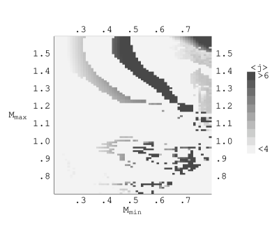
Figure 10: Fit values for $\langle j_{\mathcal{P}}\rangle$ over a set of different fitting ranges $(\mathcal{M}_{\mathrm{min}},\mathcal{M}_{\mathrm{min}})$; $\sigma=.1$ here.

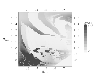
Figure 11: Fit qualities as measured by the inverse of the mean squared deviations between the simulated data and the fit; $\sigma=.1$ here. The highest fit quality appears at $(.44,.92)$.

References

- [1] R. Judson, H. Rabitz, Phys. Rev. Lett. 68, 1500 (1992).
- [2] R. Levis, G. Menkir, H. Rabitz, Science 292, 709 (2001).
- [3] A. Assion et al., Science, 282, 919 (1998).
- [4] S. Vajda et al., Chem. Phys., 267, 231 (2001).
- [5] J. Kunde et al., Appl. Phys. Lett. 77, 924 (2000).
- [6] R. Bartels et al., Nature 406, 164 (2000).
- [7] C. Bardeen et al., Chem. Phys. Lett. 280, 151 (1997).
- [8] T. Weinacht, J. White, P. Bucksbaum, J. Chem. A 103, 10166 (1999).
- [9] M. Dahleh, A. Peirce, H. Rabitz, Phys. Rev. A 37, 4950 (1988).
- [10] R. Kosloff et al., Chem. Phys. 139, 201 (1989).
- [11] H. Rabitz, W. Zhu, Accts. Chem. Res. 33, 572 (2000).
- [12] S. Rice, M. Zhao, Optical Control of Molecular Dynamics, Wiley (2000).
- [13] An alternative scheme quantifies pathway importance by associating to each pathway not a probability but rather an amplitude and a phase (A. Mitra and H. Rabitz, to be published). Although this latter scheme was not originally formulated in terms of dynamical trajectories, the amplitudes correspond in some sense to the trajectory probabilities that result from the jump rule , which does not preserve (6).
- [14] Optimization results provided by A. Mitra.
- [15] D. Bohm, Phys. Rev. 85, 166 (1952); Phys. Rev. 85, 180 (1952).
- [16] J. Bell, “Beables for quantum field theory,” Speakable and unspeakable in quantum mechanics, Cambridge University Press (1987).
- [17] The definition of as interaction picture states has the affect of eliminating larger contributions to the jump probabilities from the terms, hence reducing the overall frequency of jumps. Had we taken as Schrodinger picture states, we would have had to decrease the time step by a factor for comparable results. This factor is around 10 for the model 7-level system.
- [18] G. Bacciagaluppi, Found. Phys. Lett. 12 1 (1999), quant-ph/9811040.