Multipartite entanglement and quantum state exchange

Abstract

We investigate multipartite entanglement in relation to the process of quantum state exchange. In particular, we consider such entanglement for a certain pure state involving two groups of $N$ trapped atoms. The state, which can be produced via quantum state exchange, is analogous to the steady-state intracavity state of the subthreshold optical nondegenerate parametric amplifier. We show that, firstly, it possesses some $2N$-way entanglement. Secondly, we place a lower bound on the amount of such entanglement in the state using a novel measure called the entanglement of minimum bipartite entropy.

I Introduction

Multipartite entanglement is entanglement that crucially involves three or more particles. A well-known example of it occurs in the generalized GHZ state $|\psi\rangle=|0\rangle^{\otimes M}+|1\rangle^{\otimes M}$, where $M$ is an integer greater than two. Multipartite entanglement is an interesting quantum resource for a number of reasons. Firstly, it is a key resource in quantum computation as i) it has been proved that it is a necessary ingredient in order for a quantum computation to obtain an exponential speed-up over classical computation jozsa01 and ii) it is central to quantum error correction which uses it to encode states, to detect errors and, ultimately, to help implement fault-tolerant quantum computation (see, for example, Chapter 10 of nielsen00 ). The second reason why multipartite entanglement is interesting is that it can manifest nonclassical correlations such as GHZ-type correlations zukowski99 . Finally, it has been conjectured that multipartite entangled states contain a wealth of interesting and unexplored physics preskill .

In order to quantify the amount of multipartite entanglement present in a state, a number of measures have been proposed. Firstly, Vedral et al. vedral97 have suggested a measure of multipartite entanglement for a state $\rho$ which is the minimum relative entropy between $\rho$ and any separable state. For systems with more than two subsystems, they defined a separable state as one in which the state of at least one subsystem can be factored out from that of the others. In addition, Coffman, Kundu and Wootters coffman00 have extended the bipartite entanglement measure called the tangle wootters98 to the 3-tangle which measures 3-way GHZ-type entanglement. Furthermore, Vidal vidal00 has studied entanglement monotones — quantities whose magnitudes do not increase on average under local transformations — and has proposed that all of them can be regarded as entanglement measures. Meyer and Wallach meyer01 have proposed a measure of “global entanglement” for $n$-qubit pure states which is the sum of a number of terms involving wedge products. Each wedge product involves computational-basis expansion coefficients for various $(n-1)$-qubit states obtained by deleting a qubit from the state of interest. Similarly, Wong and Anderson n_tangle have extended the tangle to an arbitrary even number of qubits for pure states. Finally, Biham, Nielsen and Osborne biham01 have proposed the Groverian entanglement for a pure state $|\psi\rangle$ based on how successful Grover’s algorithm grover96 performs given the input $|\psi\rangle$. The Groverian entanglement is equivalent to a measure in vedral97 , however, it shows an interesting link between an entanglement measure and the quantum information processing capability of states. In addition to the measures listed above a number of others have also been proposed.

Quantum state exchange parkins1 ; parkins2 ; parkins4 ; parkins3 ; parkins5 is a newly formulated process by which information is transferred from an electromagnetic field to the vibrational state of one or more trapped atom(s). It is implemented using a stimulated Raman process that couples the electromagnetic field to the vibrational state and thus transfers information from the former to the latter. We explain it in more detail in Section II.

In this paper we show that quantum state exchange can be used to create an entangled state for $2N$ trapped atoms that is a useful quantum resource. We begin in, Subsection II.1, by explaining the process of quantum state exchange via presenting a detailed example of it within a simple system consisting of a harmonically trapped atom interacting with a cavity mode. Next, Subsection II.2 shows that quantum state exchange can be used to generate an entangled pure state for two groups of $N$ trapped atoms located in two spatially separated far-off-resonance dipole-force traps (FORTs). In Subsection II.3 we present a detailed summary of the remainder of the paper. Sections III and IV then investigate the nature of the state’s $2N$-way entanglement. That is, the nature of its entanglement that spans across all $2N$ atoms. In particular, in Subsections III.1 and IV we qualitatively explore this entanglement by presenting a novel necessary and sufficient condition for the presence of $M$-way entanglement for $M$-partite pure states and then showing that the state satisfies it. In Section IV we quantitatively explore the state’s $2N$-way entanglement by first presenting a novel multipartite entanglement measure for pure states in Subsection IV.1. This measure is based on the von Neumann entropies nielsen00 ; preskill98 for all the reduced density operators obtainable from some pure state of interest by tracing over some of the subsystems for the state. After defining the measure, we then use it to calculate lower bounds on the amount of $2N$-way entanglement in the state in Subsection IV.2. Finally, we discuss our results in Section V.

II Background theory

II.1 Quantum state exchange

Perhaps the simplest system in which quantum state exchange can occur parkins1 involves a two-level atom confined within a harmonic trap which, in turn, lies inside a linearly damped optical cavity with one lossy mirror and one ideal one. The atom’s vibrational motion is described by the annihilation operators $b_{x},b_{y}$ and $b_{z}$. The two-level atom, which has a transition frequency of $\omega_{a}$, couples to both an intracavity electromagnetic field mode of frequency $\omega_{c}$ described by the annihilation operator $a$ and an external laser of frequency $\omega_{L}$. The cavity and external laser frequencies are chosen so as to drive Raman transitions that couple adjacent atomic vibrational levels. Furthermore, the cavity’s axis coincides with the $x$-axis whilst the external laser’s beam is perpendicular to this axis. Lastly, we assume that the harmonic trap is centred on a cavity-field node and thus a schematic diagram of this system is as in Fig. 1.

Figure 1: Schematic diagram of a simple system in which quantum state exchange can occur. A two-level atom (represented by a black circle) lies within a harmonic trap that is itself inside an optical cavity. The cavity, which is aligned along the $x$-axis, supports a mode of frequency $\omega_{c}$ and has one lossy mirror (with damping constant $\kappa$) and one ideal one. An external laser of frequency $\omega_{L}$ is incident from a direction perpendicular to the $x$-axis.

The system’s Hamiltonian is, in a reference frame rotating at frequency $\omega_{L}$,

$$H_{\rm total}^{\rm single} = H_{\rm sys}+\kappa(aR^{{\dagger}}+a^{{\dagger}}R)+H_{\rm res},$$ (1)

where $H_{\rm res}$ is the free Hamiltonian of the reservoir coupled to the cavity mode, $\kappa$ is a damping rate, $R$ is a reservoir operator and $H_{\rm sys}$ is the Hamiltonian for the cavity-atom system which is

$$H_{\rm sys} = \Sigma_{j=x,y,z}\hbar\nu_{j}(b^{{\dagger}}_{j}b_{j}+1/2)+\hbar\delta a^{{\dagger}}a+\hbar\Delta\sigma_{+}\sigma_{-}$$ (2)

$$+\hbar\big{[}{\cal E}_{L}(y,z,t)\sigma_{+}+{\cal E}^{*}_{L}(y,z,t)\sigma_{-}\bigr{]}$$

$$+\hbar g_{0}\sin(kx)\bigl{(}a^{{\dagger}}\sigma_{-}+a\sigma_{+}\bigr{)},$$

where $\nu_{x},\nu_{y}$ and $\nu_{z}$ are the harmonic-oscillator frequencies along the trap’s $x$, $y$ and $z$ axes, $\sigma_{+}$ and $\sigma_{-}$ are atomic raising and lowering operators for the two-level atom, $\delta=\omega_{c}-\omega_{L}$, $\Delta=\omega_{a}-\omega_{L}$, ${\cal E}_{L}$ is the complex amplitude of the external laser field, $k=2\pi/\lambda$, where $\lambda=2\pi c/\omega_{c}$, $x=\sqrt{\hbar/2m\nu_{x}}(b_{x}+b_{x}^{{\dagger}})$, where $m$ is the mass of the two-level atom, and $g_{0}$ ($g_{0}\in\mathbb{R}$) is the coupling constant for the atom-field interaction. Observe that $\omega_{c}-\omega_{L}=\nu_{x}$.

The following reasonable assumptions are made about the system so as to make calculations involving it more tractable:

1. The cavity field and external laser frequencies are appreciably detuned from $\omega_{a}$ and the two-level atom is initially in the ground state. Thus, the excited internal state is sparsely populated and spontaneous emission effects are negligible and can be ignored.

2. Vibrational decoherence occurs over a timescale much longer than that of the interaction producing quantum state exchange, as is the case in an ion-trap realization of the system parkins1 . Consequently, it has a minimal effect over our timescale of interest and is ignored.

3. The trap dimensions are small compared to the cavity mode wavelength and thus $\sin(kx)\ll 1$. It follows from this that $\sin kx\simeq\eta_{x}(b_{x}+b_{x}^{{\dagger}})$, where $\eta_{x}=k\sqrt{\hbar/2m\nu_{x}}$. It also follows that we can arrange things so that the $y$ and $z$ dependence of the external laser field is negligible and thus, assuming ${\cal E}_{L}$ is time independent, that ${\cal E}_{L}(y,z,t)\simeq{\cal E}e^{-i\phi_{L}}$, where ${\cal E}$ is a real time-independent amplitude.

4. The damping parameter $\kappa$ is such that $\nu_{x}\gg\kappa\gg g_{0}\eta_{x}{\cal E}/\Delta$.

Given the assumptions above, and also assuming that $g^{2}_{0}/\Delta\ll\delta$ and $g_{0}\langle a^{{\dagger}}a\rangle\ll{\cal E}_{L}$, $H_{\rm total}^{\rm single}$ can be rewritten as parkins5 (p. 012308)

$$H_{\rm total}^{\rm single} = \Sigma_{j=x,y,z}\hbar\nu_{j}\left(b_{j}^{{\dagger}}b_{j}+1/2\right)+\hbar\delta a^{{\dagger}}a-\frac{\hbar{\cal E}^{2}}{\Delta}$$ (3)

$$-\frac{\hbar g_{0}{\cal E}}{\Delta}\sin(kx)\left(a^{{\dagger}}e^{-i\phi_{L}}+ae^{i\phi_{L}}\right)$$

$$+\kappa(aR^{{\dagger}}+a^{{\dagger}}R)+H_{\rm res}$$

by adiabatically eliminating the evolution of the internal states. Furthermore, for the system under consideration, it has been shown parkins1 that, in the steady-state regime, the vibrational state of the atom in the $x$ direction is solely determined by the input field (i.e. the light field entering the cavity) such that

$$\tilde{b}_{x}(\omega)=\frac{\sqrt{2\Gamma}}{i\omega-\Gamma}\tilde{a}_{\rm in}(\omega),$$ (4)

where $\tilde{b}(\omega)=\frac{1}{\sqrt{2\pi}}\int_{t=-\infty}^{\infty}dtb_{x}(t)e^{i\left(\nu_{x}-\omega\right)t}$, $\Gamma=g_{0}^{2}\eta_{x}^{2}{\cal E}^{2}/\left(\Delta^{2}\kappa\right)$ and $\tilde{a}_{\rm in}(\omega)=\frac{1}{\sqrt{2\pi}}\int_{t=-\infty}^{\infty}dte^{-i\omega t}\tilde{a}_{\rm in}(t)$, where $\tilde{a}_{\rm in}(t)=\frac{1}{\sqrt{2\pi}}\int_{\omega^{\prime}=-\infty}^{\infty}d\omega^{\prime}e^{i\left(\nu_{x}-\omega^{\prime}\right)t}c_{0}(\omega^{\prime})$, where $c_{0}(\omega^{\prime})$ is the value of the reservoir annihilation operator for the frequency $\omega^{\prime}$ at time $t=0$. The proportionality between $\tilde{b}_{x}(\omega)$ and $\tilde{a}_{\rm in}(\omega)$ present in Eqn (4) denotes that the “statistics of the input field [have been] …‘written onto’ the state of the oscillator” parkins1 (p. 498) (i.e. onto the atom’s vibrational state in the $x$ direction). We thus say that quantum state exchange has taken place when this equation holds.

II.2 System of interest

In this paper we use quantum state exchange to generate a particular state involving two groups of $N$ trapped atoms which we later show contains multipartite entanglement that is a useful quantum resource. Our work follows on from parkins2 in which it was asserted that for a certain system consisting of two groups of $N$ trapped atoms, quantum state exchange could generate “a highly entangled state of all 2[N] atoms”. The system we consider can be seen as a concrete example of that described in the last paragraph of parkins2 — our main original contributions are, firstly, demonstrating that the state within our system is a multipartite entangled one and, secondly, quantitatively analysing the multipartite entanglement within it.

The system we consider comprises of, firstly, a subthreshold nondegenerate optical parametric amplifier (NOPA) ou92a ; ou92b ; kimble92 for which the two external output fields first pass through Faraday isolators and then each feed into a different linearly damped optical cavity for which one mirror is perfect and the other is lossy. The axes of both cavities coincide with the $x$-axis. Each cavity supports an electromagnetic field mode of frequency $\omega_{jc}$ that is described by the annihilation operator $a_{j}$, where $j$ enumerates the cavities. Within the $j^{\rm th}$ cavity lie $N$ identical two-level atoms which each possess an internal transition frequency of $\omega_{a}$. These are trapped in a linear configuration parallel to the $x$-axis by, firstly, a one-dimensional far-off-resonance dipole-force trap (FORT) miller93 ; lee96 . This consists of cavity mode of frequency $\omega_{T}$ which exhibits a standing-wave pattern along the $x$-axis. The frequency $\omega_{T}$ is strongly detuned from all atomic resonant frequencies and thus the cavity mode’s field exerts dipole forces on the atoms, trapping each of them near a separate node of the field. In addition, the FORT’s axis is parallel to the $x$-axis and it thus traps the atoms in the $x$ direction. The atoms are also tightly confined in the $y$ and $z$ directions by a two-dimensional far-off resonance optical lattice jessen96 ; haycock97 ; deutsch98 and thus move negligably in these directions. The combined effect of all the trapping fields is to confine each atom in its own one-dimensional trap parallel to the $x$-axis. Furthermore, the atoms are located such that the mean position of each atom coincides with a node of the cavity field described by $a_{j}$. The annihilation operator $b_{jx}^{(m)}$ describes the vibrational motion of the $m^{\rm th}$ atom in the $j^{\rm th}$ trap in the $x$ direction. Finally, external lasers of frequency $\omega_{L}$ whose beams are perpendicular to the $x$-axis are incident on all atoms and thus Fig. 2 illustrates the system under consideration.

Figure 2: Schematic diagram for a system involving, firstly, a subthreshold optical nondegenerate parametric amplifier (NOPA) whose output modes pass through Faraday isolators (represented by an F enclosed in a circle) and then feed into linearly damped optical cavities (as indicated by the sinusoidal curves inside both cavites which represent the cavity modes $a_{1}$ and $a_{2}$). These cavities are aligned along the $x$-axis and both have one ideal mirror and one lossy one (with damping constant $\kappa$). Inside each of them is a far-off-resonance dipole-force trap (FORT) that, along with a two-dimensional far-off resonance optical lattice, confines $N$ identical two-level atoms in linear chain parallel to the $x$-axis. Observe that the FORTs’ trapping modes are not shown in the diagram. External lasers of frequency $\omega_{L}$ are incident on each atom in both traps from a direction perpendicular to the $x$-axis.

The Hamiltonian for the $j^{\rm th}$ optical cavity and the $N$ atoms within it is

$$H_{\rm j\>total} = H_{j0}^{\rm atom}+H_{j0}+H_{jI}$$ (5)

$$+\kappa(a_{j}R^{{\dagger}}_{j}+a^{{\dagger}}_{j}R_{j})+H_{\rm j\>res},$$

where $H_{j0}^{\rm atom}$ is the free Hamiltonian for the vibrational states of the atoms and $H_{j0}$ is the free Hamiltonian for the cavity field and the atoms’ internal states. The term $H_{jI}$ is the interaction Hamiltonian describing the Raman processes involving the cavity field, the external lasers and the atoms. To be more specific, $H_{j0}^{\rm atom}=\hbar\nu_{jx}\sum_{m=1}^{N}\left(b_{jx}^{(m)\>{\dagger}}b_{jx}^{(m)}+\frac{1}{2}\right)$, where $\nu_{jx}$ is the vibrational frequency of the FORT in the $j^{\rm th}$ cavity (which we call the $j^{\rm th}$ FORT) in the $x$ direction. This frequency is equal to $\omega_{jc}-\omega_{L}$. The Hamiltonian $H_{j0}$ is, in a frame rotating at frequency $\omega_{L}$,

$$H_{j0}=\hbar\delta a_{j}^{{\dagger}}a_{j}+\hbar\Delta\sum_{m=1}^{N}\sigma_{j+}^{(m)}\sigma_{j-}^{(m)},$$ (6)

where $\delta_{j}=\omega_{jc}-\omega_{L}$, $\Delta=\omega_{a}-\omega_{L}$ and $\sigma_{j+}^{(m)}$ and $\sigma_{j-}^{(m)}$ are raising and lower operators for the internal states of the $m^{\rm th}$ atom in the $j^{\rm th}$ trap. The term $H_{jI}$ is

$$H_{jI} = \hbar\sum_{m=1}^{N}{\cal E}_{L}(y,z,t)\sigma_{j+}^{(m)}+{\cal E}^{*}_{L}(y,z,t)\sigma_{j-}^{(m)}$$ (7)

$$+\hbar g_{0}\sum_{m=1}^{N}\sin(k_{j}x_{jm})\bigl{(}a^{{\dagger}}_{j}\sigma_{j-}^{(m)}+a_{j}\sigma_{j+}^{(m)}\bigr{)},$$

where ${\cal E}_{L}$ is the complex amplitude for all external lasers, $k_{j}=\omega_{jc}/c$ and $g_{0}$ ($g_{0}\in\mathbb{R}$) is the coupling constant for the atom-field interaction. Finally, $H_{\rm j\>res}$ is the Hamiltonian for the external reservoir that couples to the $j^{\rm th}$ cavity for which $R_{j}$ is a reservoir annihilation operator and $\kappa$ is a damping constant.

The feasible assumptions below are made about the system in order to simplify calculations for it and to focus on its most important aspects:

1. The cavity field and external laser frequencies are appreciably detuned from $\omega_{a}$ and all two-level ions are initially in the ground state. Thus, the excited internal states are sparsely populated and spontaneous emission effects are negligible and can be ignored.

2. Vibrational decoherence occurs over a timescale much longer than that of the interactions producing quantum state exchange and consequently can be ignored.

3. The wavelength of the cavity mode described by $a_{j}$ is much greater than the distance that any atom in the $j^{\rm th}$ trap strays from the cavity-field node about which it is trapped. Thus, $\sin(kx_{jm})\simeq kx_{jm}<<1$ and hence all atoms experience a potential that is, to a good approximation, harmonic. This justifies the form of $H_{j0}^{\rm atom}$.

4. All atoms are tightly confined in the $y$ and $z$ directions. This allows us to ignore the $y$ and $z$ dependence of the external laser fields and thus, assuming ${\cal E}_{L}$ is time independent, it follows that ${\cal E}_{L}(y,z,t)\simeq{\cal E}e^{-i\phi_{L}}$, where ${\cal E}$ is a real time-independent amplitude.

5. The damping parameter $\kappa$ is such that $\nu_{jx}\gg\kappa\gg g_{0}\eta_{jx}\sqrt{N}{\cal E}/\Delta$, where $\eta_{jx}=k_{j}\sqrt{\hbar/2m\nu_{jx}}$, where $m$ is the mass of each atom.

Given the assumptions above, we can write $H_{\rm j\>total}$ in terms of normal-mode creation and annihilation operators (by adiabatically eliminating the evolution of the internal states) as

$$H_{\rm j\>total} = \hbar\sum_{m=1}^{N}\nu_{jx}\left(B_{jx}^{{\dagger}\>(m)}B_{jx}^{(m)}+\frac{1}{2}\right)+\hbar\delta a^{{\dagger}}a$$ (8)

$$- \frac{\hbar N{\cal E}^{2}}{\Delta}-\frac{\hbar g_{0}\eta_{jx}\sqrt{N}{\cal E}}{\Delta}\times$$

$$\left(\sum_{m=1}^{N}(B_{jx}^{(m)}+B_{jx}^{(m)\>{\dagger}})\bigl{(}a^{{\dagger}}_{j}e^{-i\phi_{L}}+a_{j}e^{i\phi_{L}}\bigr{)}\right)$$

$$+ \kappa(a_{j}R^{{\dagger}}_{j}+a^{{\dagger}}_{j}R_{j})+H_{\rm j\>res},$$

where $B_{jx}^{(m)}$ is the annihilation operator for the $m^{\rm th}$ normal mode for the $j^{\rm th}$ trap in the $x$ direction. For example, $B_{jx}^{(1)}$ is a centre-of-mass mode annihilation operator which is $B_{jx}^{(1)}=1/\sqrt{N}\left(b_{jx}^{(1)}+b_{jx}^{(2)}+\ldots b_{jx}^{(N)}\right)$ whilst $B_{jx}^{(2)}$ is the annihilation operator for the breathing mode which is $B_{jx}^{(2)}=1/\sqrt{2}\left(-b_{jx}^{(1)}+b_{jx}^{(2)}\right)$ when $N=2$.

Comparing Eqn (8) to Eqn (3), we see that $B_{jx}^{(1)}$ in Eqn (8) plays an almost identical role to that of $b_{x}$ in Eqn (3). Given that $\sin(kx)\simeq\eta_{x}(b_{x}+b_{x}^{{\dagger}})$ in Eqn (3), the only difference between the forms in which the two operators appear results from a factor of $\sqrt{N}$ appearing in front of ${\cal E}$ in Eqn (8). As a consequence, $B_{jx}^{(1)}$ in Eqn (8) couples to the cavity mode $a_{j}$ identically — aside from the factor of $\sqrt{N}$ — to the manner in which $b_{x}$ couples to $a$. It follows that as quantum state exchange takes place in the system described by $H_{\rm total}^{\rm single}$ with information about an input electromagnetic field being transferred to $b_{x}$, it also occurs in the system described by $H_{\rm j\>total}$ due to the correspondence between the two system’s Hamiltonians. Thus, in the latter system, information about the input field is transferred to the centre-of-mass mode for the trapped atoms in the $x$ direction just as if this mode was a vibrational mode for a single harmonically trapped atom. The only difference between the $N$-atom case and one described by $H_{\rm total}^{\rm single}$ is that the effective coupling in the former case is increased by a factor of $\sqrt{N}$. This conclusion can also be verified via comparing the Langevin equations for $B_{jx}^{(m)}$ and $b_{x}$. Due to symmetry considerations, collective modes other than the centre-of-mass modes do not absorb any photons in modes $a_{1}$ and $a_{2}$. Thus, assuming these other modes are initially in vacuum states, they remain so during quantum state exchange.

In parkins2 , it was shown that we can transfer the intracavity steady-state for the subthreshold nondegenerate parametric amplifier which is

$$|\psi\rangle=\frac{1}{\cosh r}\Sigma_{n=0}^{\infty}\tanh^{n}r|n\rangle_{\rm 1}|n\rangle_{\rm 2},$$ (9)

where the subscripts 1 and 2 denote the two output modes and $r$ is a real squeezing parameter, into the vibrational states in the $x$ direction for two single trapped atoms in different harmonic traps. Using the correspondence between the quantum state exchange processes involving a single harmonically trapped atom and $N$ harmonically trapped atoms demonstrated above, it follows that in the system illustrated in Fig. 2 we can transfer $|\psi\rangle$ into the centre-of-mass modes in the $x$ direction for the two sets of $N$ trapped atoms thus producing, in the steady state,

$$|\psi_{\rm CM}\rangle=\frac{1}{\cosh r}\Sigma_{{\cal N}=0}^{\infty}\tanh^{{\cal N}}r|{\cal N}\rangle_{1}|{\cal N}\rangle_{2},$$ (10)

where $|{\cal N}\rangle_{j}$ denotes the centre-of-mass vibrational number state for the $x$ direction with eigenvalue ${\cal N}$ for the atoms in the $j^{\rm th}$ FORT. In writing this state we have omitted the states of collective modes other than the centre-of-mass modes as we have assumed these other modes are in vacuum states throughout the quantum state exchange process.

Importantly, the process of creating $|\psi_{\rm CM}\rangle$ just outlined does not seem to be overly experimentally infeasible. This is so as optical cavities and nondegenerate optical parametric amplifiers have been widely realized quantum optical laboratories for some time. In addition, neutral atoms have been confined within standing-wave dipole-force traps that, in turn, lie within optical cavities van_enk01 . Relatedly, experiments in which a single harmonically trapped ion has been placed within an optical cavity have been conducted mundt02 .

II.3 Summary

In this paper, we explore multipartite entanglement in relation to quantum state exchange and in Section III, follow on from a multipartite entanglement condition implicit in work by Dür and Cirac dur_cirac by presenting a novel condition. The satisfaction of this novel condition implies that any pure state comprising of $M$ subsystems is $M$-way entangled. Here, an $M$-way entangled state is one possessing entanglement that spans across $M$ subsystems as does the generalized GHZ state $|\psi\rangle=|0\rangle^{\otimes M}+|1\rangle^{\otimes M}$. After presenting this condition, we then use it to show qualitatively that $|\psi_{\rm CM}\rangle$ is $2N$-way entangled. In Section IV, we quantitatively consider the entanglement in $|\psi_{\rm CM}\rangle$. We introduce a novel multipartite entanglement measure for pure states we call the entanglement of minimum bipartite entropy or $E_{\rm MBE}$ which is the minimum of the von Neumann entropies of all the reduced density operators obtainable from some pure state of interest by tracing over some of the subsystems for the state. After this, we use $E_{\rm MBE}$ to calculate a lower bound for the amount of 4-way, 6-way and 8-way entanglement in $|\psi_{\rm CM}\rangle$ for $N=2,3,4$ respectively for a range of $r$ values. Finally, we discuss the nature of our results.

It is interesting to investigate the nature $|\psi_{\rm CM}\rangle$’s $2N$-way entanglement for a number of reasons. Firstly, it has been claimed — but not demonstrated — $|\psi_{\rm CM}\rangle$ is “entangled state of all 2[$N$] …atoms” parkins1 . It is thus interesting to investigate $|\psi_{\rm CM}\rangle$’s $2N$-way entanglement in order to see if this implied claim is true. Secondly, it is interesting to investigate $|\psi_{\rm CM}\rangle$’s $2N$-way entanglement as it is a massive-particle state which is important as, to date, mostly massless photons have been used to experimentally investigate entanglement. Thirdly, if the claim is true, then it means that $|\psi_{\rm CM}\rangle$ is a state consisting of $2N$ entangled harmonic oscillators, each possessing an infinite-dimensional Hilbert space as opposed to the two-dimensional Hilbert space of a qubit, that is $2N$-way entangled.

III Qualitative results

III.1 Negative partial transpose sufficient condition

Assume that, for a certain state $\rho$, we wish to know the answer to the question “Does $\rho$ contain at least some $M$-way entanglement?” Whilst answering this question does not tell us everything about the nature of $\rho$’s $M$-way entanglement, it nevertheless tells us something of interest. One way to answer it, provided that $\rho$ consists of qubits, is to use a condition that can be readily derived from work by Dür and Cirac dur_cirac . This condition involves negative partial transposes (NPTs) peres96 ; horodecki96 ; horodecki97 and thus we name it the NPT sufficient condition. It is sufficient for the presence of $M$-way entanglement for all $\rho$’s consisting of $P$ qubits, where $P\geq M$, and is based on generalizing the notions of separability and inseparability to many-qubit systems. Before stating the condition, it is first useful to mention two things. Firstly, we define an M-partite split of $\rho$ dur_cirac to be a division or split of $\rho$ into $M$ parts which each consist of one or more subsystems. Secondly, we observe that $\rho$ can always be converted to a state that is diagonal in a certain basis by a “depolarization” process consisting of particular local operations dur_cirac . This basis consists of $M$-qubit generalized GHZ states of the form $|\psi\rangle=1/\sqrt{2}\left(|j\rangle|0\rangle\pm|2^{N-1}-j-1\rangle|1\rangle\right)$, where $j$ is a natural number that we write in binary as $M-1$ bits, i.e. $j\equiv j_{1}j_{2}\ldots j_{M-1}$, where $j_{x}$ is the $x^{\rm th}$ bit in $j$’s binary representation. Given these two things, the NPT sufficient condition states that $\rho$ is $M$-way entangled for a given $M$-partite split if the diagonal state that it depolarizes to is such that all bipartite splits that contain the $M$-partite split have negative partial transposes. A bipartite split is one that divides a system into two parts, i.e. a $2$-partite split. Also, a bipartite split that contains an $M$-partite split is one that does not separate members of any of the $M$ subsystems onto two different sides of the bipartite split. That is, one that does not cross any of the divisions created by the $M$-partite split.

III.2 Result

Following on from the NPT sufficient condition, we propose a necessary and sufficient condition for the existence of $M$-way entanglement for $M$-partite pure states. Our condition is based on the traces of the squares of reduced density matrices obtained by tracing over some of the subsystems constituting our system of interest. After formulating it, we then use it to demonstrate that $|\psi_{\rm CM}\rangle$ contains some $2N$-way entanglement. Our motivations for employing our condition instead of the NPT sufficient condition are that i) it seems to be mathematically simpler to calculate whether or not our condition is satisfied and ii) as we are concerned with a pure state, our condition is stronger than the NPT sufficient condition in the sense that it is both necessary and sufficient as opposed to just being sufficient.

Our $M$-way entanglement condition utilizes the fact that when a pure state $|\psi\rangle$ for $M$ subsystems is $M$-way entangled then we cannot write it as $|\psi\rangle=|\phi_{1}\rangle_{Q_{j}}\otimes|\phi_{2}\rangle_{\bar{Q}_{j}}$, where $|\phi_{1}\rangle_{Q_{j}}$ and $|\phi_{2}\rangle_{\bar{Q}_{j}}$ are the states for the subsystems denoted by $Q_{j}$ and ${\bar{Q}_{j}}$ respectively and both $Q_{j}$ and ${\bar{Q}_{j}}$ denote at least one subsystem. To put this another way, when $|\psi\rangle$ is $M$-way entangled then there is no way to represent it as the tensor product of two pure states. Consequently, excluding all such possibilities suffices to show, and is also, in general, necessary to show, that $|\psi\rangle$ is $M$-way entangled. This can be done by first checking that no single-subsystem state can be factored out from the state of the remaining $M-1$ subsystems. We do this by checking that the traces of the squares of all the reduced density operators obtainable from $|\psi\rangle$ by tracing over one subsystem are less than one. That is, that $Tr([\rho_{Q_{j}}]^{2})<1$, where $\rho_{Q_{j}}$ is the reduced density operator obtained from $|\psi\rangle\langle\psi|$ by tracing over the subsystem denoted by $Q_{j}$ for all $Q_{j}$ denoting just one subsystem. We can then repeat this procedure, considering all $Q_{j}$’s corresponding to all pairs of subsystems, then all triples and so forth until we have considered all $Q_{j}$’s corresponding to all sets of $R$ subsystems, where $R=\lfloor M/2\rfloor$, where $\lfloor x\rfloor$ is the largest integer less than or equal to $x$. It is sufficient to only consider sets of up to those corresponding to $\lfloor M/2\rfloor$ subsystems as a necessary condition for being able to factor out any larger a number of subsystems from $|\psi\rangle$ is the ability to also factor out $\lfloor M/2\rfloor$ or fewer subsystems. Underlying the process just described is that of seeing whether or not we can exclude all the ways that $|\psi\rangle$ could fail to be $M$-way entangled.

Our condition can be formalized as Definition 1 which is as follows:

Definition 1 : For a pure state $|\psi\rangle$ for $M$ subsystems, consider the set $Q$ whose members $Q_{j}$ are themselves sets of subsystems for the system corresponding to $|\psi\rangle$. This set $Q$ contains all sets of $P$ subsystems for this system, where $1\leq P\leq\lfloor M/2\rfloor$. Given this, $|\psi\rangle$ is $M$-way entangled iff, for all $Q_{j}$, $Tr\left([\rho_{Q_{j}}]^{2}\right)<1$, where $\rho_{Q_{j}}$ is the reduced density operator obtained by beginning with $|\psi\rangle\langle\psi|$ and tracing over the subsystems $Q_{j}$.

To illustrate Definition 1 consider, for example, the GHZ state $|\psi\rangle_{\rm GHZ}=1/\sqrt{2}\left(|000\rangle_{123}+|111\rangle_{123}\right)$, where the subscripts 1, 2 and 3 denote subsystems of $|\psi\rangle_{\rm GHZ}$. The parameter $P=\lfloor 3/2\rfloor=1$ and consequently the set $Q$ comprises of all sets of one subsystem and thus $Q=\{\{1\},\{2\},\{3\}\}$, where the numbers again denote subsystems for $|\psi\rangle_{\rm GHZ}$. For the element $\{1\}$, for example, $Tr([\rho_{\{1\}}]^{2})=1/2$. Calculating $Tr([\rho_{Q_{j}}]^{2})$ for all of $Q$’s other elements, we find that it is 1/2 in all three cases. Thus, $|\psi\rangle_{\rm GHZ}$ satisfies Definition 1 and hence is said to be 3-way entangled, as is the case.

To further explain Definition 1, we now apply it to determining whether the following four-party states are 4-way entangled :

1. ) $\;|\psi_{4}^{(1)}\rangle=1/\sqrt{2}\bigl{(}|0000\rangle_{1234}+|1111\rangle_{1234}\bigr{)}$,

2. ) $\;|\psi_{4}^{(2)}\rangle=1/\sqrt{2}|0\rangle_{1}\otimes(|000\rangle_{234}+|111\rangle_{234})$

3. ) $\;|\psi_{4}^{(3)}\rangle=|\phi^{+}\rangle_{12}\otimes|\phi^{+}\rangle_{34}$.

Turning to 1.), we see that upon tracing over any single subsystem, we produce a reduced density operator of the form $\rho_{Q_{j}}=1/2(|000\rangle\langle 000|+|111\rangle\langle 111|)$ for which $Tr([\rho_{Q_{j}}]^{2})=1/2$. Similarly, tracing over any two subsystems produces a density operator of the form $\rho_{Q_{j}}=1/2(|00\rangle\langle 00|+|11\rangle\langle 11|)$ for which, again, $Tr([\rho_{Q_{j}}]^{2})=1/2$. Thus, Definition 1 gives the correct result that $|\psi_{4}^{(1)}\rangle$ is 4-way entangled. For 2.), tracing over the first subsystem produces $|\psi_{4}^{(3)}\rangle=1/\sqrt{2}\bigl{(}|000\rangle_{234}+|111\rangle_{234}\bigr{)}$, which is a pure state and hence $Tr([\rho_{Q_{j}}]^{2})=1$ for the corresponding $j$. Consequently, Definition 1 tells us that $|\psi_{4}^{(2)}\rangle$ is not $4$-way entangled, as is the case. For 3.), tracing over any one subsystem produces the mixed state $\rho=I/2\otimes|\phi^{+}\rangle_{34}\langle\phi^{+}|$ and so we might be tempted to infer that $|\psi_{4}^{(3)}\rangle$ is 4-way entangled. However, when we trace over subsystems 1 and 2 or subsystems 3 and 4 we produce the pure state $|\phi^{+}\rangle$ for which $Tr\left([|\phi^{+}\rangle\langle\phi^{+}|]^{2}\right)=1$. Hence, Definition 1 correctly tells us that $|\psi_{4}^{(3)}\rangle$ is not 4-way entangled.

In applying Definition 1 to $|\psi_{\rm CM}\rangle$, we first write $|\psi_{\rm CM}\rangle$ in terms of vibrational number states for the $2N$ atoms involved as we wish to see if they are $2N$-way entangled. As a step towards doing so, upon observing that $|{\cal N}\rangle_{j}=\left(\left(B^{(1)\>{\dagger}}_{jx}\right)^{\cal N}/\sqrt{{\cal N}!}\right)|0\rangle_{j}$, we express $|{\cal N}\rangle_{j}$ in terms of vibrational number states in the $x$ direction for individual atoms as

$$|{\cal N}\rangle_{j}=\sum_{{\rm a.c.}(\vec{n},{\cal N})}c(\vec{n},{\cal N})|\vec{n}\rangle_{j},$$ (11)

where $\vec{n}$ is the $N$-component vector $(n_{1},n_{2}\ldots n_{N})$, the state $|\vec{n}\rangle_{j}=|n_{1}\rangle_{j}\otimes|n_{2}\rangle_{j}\ldots|n_{N}\rangle_{j}$, where $|n_{k}\rangle_{j}$ denotes a number state for the $k^{\rm th}$ atom in the $j^{\rm th}$ FORT and

$$c(\vec{n},{\cal N}) = {}_{j}\langle\vec{n}|{\cal N}\rangle_{j}$$ (19)

$$= \frac{\left(\!\!\begin{array}[]{c}{\cal N}\\ n_{1}\end{array}\!\!\right)\left(\!\!\begin{array}[]{c}{\cal N}-n_{1}\\ n_{2}\end{array}\!\!\right)...\left(\!\!\begin{array}[]{c}{\cal N}-n_{1}...-n_{N-2}\\ n_{N-1}\end{array}\!\!\right)}{\sqrt{{\cal N}!\times N^{{\cal N}}}}$$

$$\times\sqrt{n_{1}!n_{2}!...n_{N}!}$$

The sum $\sum_{{\rm a.c.}(\vec{n},N)}$ denotes the sum over all combinations of $n_{1},n_{2}\ldots n_{N}$ such that $\sum_{j=1}^{N}n_{j}=N$ rice94 . Using Eqn (11) to represent $|\psi_{\rm CM}\rangle$ in terms of vibrational number states for individual atoms, we obtain

$$|\psi_{\rm CM}\rangle = \frac{1}{\cosh r}\sum_{{\cal N}=0}^{\infty}\tanh^{{\cal N}}r\left(\sum_{a.c.(\vec{n},{\cal N})}c(\vec{n},{\cal N})|\vec{n}\rangle_{1}\right)$$ (20)

$$\otimes\left(\sum_{a.c.(\vec{m},{\cal N})}c(\vec{m},{\cal N})|\vec{m}\rangle_{2}\right).$$

We now show that the right-hand side of Eqn (20) satisfies Definition 1 and thus that $|\psi_{\rm CM}\rangle$ is $2N$-way entangled. We do this by first writing $|\psi_{\rm CM}\rangle$ as the most general bipartite state possible involving vibrational number states for individual atoms. Next, we show that, upon tracing over the atoms in the half of the bipartite split containing the lesser number of atoms and then finding the trace of the square of the resulting reduced density operator, that this is less than one. It follows that, for all $j$, $Tr([\rho_{Q_{j}}]^{2})<1$. Hence, we satisfy Definition 1 and so $|\psi_{\rm CM}\rangle$ is $2N$-way entangled.

Dividing the atoms in $|\psi_{\rm CM}\rangle$ into subsystems $A$ and $B$ containing, respectively, $R$ and $2N-R$ atoms ($R\neq 0$), we can write $|\psi_{\rm CM}\rangle$ as

$$|\psi_{\rm CM}\rangle=\sum_{i=0}^{\infty}c_{i}|f_{i}\rangle_{A}\otimes|g_{i}\rangle_{B},$$ (21)

where $\||f_{i}\rangle_{A}\|=\||g_{i}\rangle_{B}\|=1$ and the $|f_{i}\rangle_{A}$, but not necessarily the $|g_{i}\rangle_{B}$, are mutually orthogonal. (As we can always write $|\psi_{\rm CM}\rangle$ in biorthogonal form peres93 , there exist $|g_{i}\rangle_{B}$ that are mutually orthogonal. However, we are not concerned with this form in the current calculation and so do not consider such a decomposition of $|\psi_{\rm CM}\rangle$.) To give an example, when $N=2$ and $A$ contains the first atom in the first trap

$$|\psi_{\rm CM}\rangle = \frac{1}{\cosh r}|0\rangle_{A}\otimes\left(|000\rangle_{B}+\frac{\tanh r}{2}|101\rangle_{B}\right.$$ (22)

$$\left.+\frac{\tanh r}{2}|110\rangle_{B}+\frac{\tanh^{2}r}{4}|202\rangle_{B}\right.$$

$$\left.+\frac{\sqrt{2}\tanh^{2}r}{4}|211\rangle_{B}+\frac{\tanh^{2}r}{4}|220\rangle_{B}+\ldots\right)$$

$$+\frac{1}{\cosh r}|1\rangle_{A}\otimes\left(\frac{\tanh r}{2}|001\rangle_{B}\right.$$

$$\left.+\frac{\tanh r}{2}|010\rangle_{B}+\frac{\tanh^{2}r}{\sqrt{8}}|102\rangle_{B}\right.$$

$$\left.+\frac{\sqrt{2}\tanh^{2}r}{2}|111\rangle_{B}+\frac{\tanh^{2}r}{2}|120\rangle_{B}+\ldots\right)$$

$$+\frac{1}{\cosh r}|2\rangle_{A}\otimes\left(\frac{\tanh^{2}r}{4}|002\rangle_{B}\right.$$

$$\left.+\frac{\sqrt{2}\tanh^{2}r}{8}|011\rangle_{B}+\frac{\tanh^{2}r}{4}|020\rangle_{B}+\ldots\right)$$

$$+\ldots,$$

where $|x\rangle_{A}=|n_{1}=x\rangle_{A}$ and $|x_{1}x_{2}x_{3}\rangle_{B}=|n_{2}=x_{1},m_{1}=x_{2},m_{2}=x_{3}\rangle_{B}$. Here, for example, $c_{0}=1/\cosh r$, $|f_{0}\rangle_{A}=|0\rangle_{A}$, $c_{1}=1/\cosh r$, $|f_{1}\rangle_{A}=|1\rangle_{A}$,

$$|g_{0}\rangle_{B} = \frac{1}{\sqrt{{\cal M}_{0}}}\left(|000\rangle_{B}+\frac{\tanh r}{2}|101\rangle_{B}\right.$$

$$\left.+\frac{\tanh r}{2}|110\rangle_{B}|\rangle+\frac{\tanh^{2}r}{4}|202\rangle_{B}\right.$$

$$\left.+\frac{\sqrt{2}\tanh^{2}r}{4}|211\rangle_{B}+\frac{\tanh^{2}r}{4}|220\rangle_{B}+\ldots\right)$$

$${\rm and}$$

$$|g_{1}\rangle_{B} = \frac{1}{\sqrt{{\cal M}_{1}}}\left(\frac{\tanh r}{2}|001\rangle_{B}+\frac{\tanh r}{2}|010\rangle_{B}\right.$$

$$\left.+\frac{\tanh^{2}r}{\sqrt{8}}|102\rangle_{B}+\frac{\sqrt{2}\tanh^{2}r}{2}|111\rangle_{B}\right.$$

$$\left.+\frac{\tanh^{2}r}{2}|120\rangle_{B}+\ldots\right),$$

where ${\cal M}_{0}$ and ${\cal M}_{1}$ normalize $|g_{0}\rangle_{B}$ and $|g_{1}\rangle_{B}$. Upon tracing over $A$ in Eqn (21) and squaring the resulting reduced density operator $\rho_{Q_{A}}$, we obtain

$$[\rho_{Q_{A}}]^{2}=\sum_{i,j=0}^{\infty,\infty}c_{i}^{2}c_{j}^{2}|g_{i}\rangle\langle g_{i}|g_{j}\rangle\langle g_{j}|.$$ (23)

Calculating the trace of $[\rho_{Q_{A}}]^{2}$ yields

$$Tr\left([\rho_{Q_{A}}]^{2}\right)=\sum_{i,j=0}^{\infty,\infty}c_{i}^{2}c_{j}^{2}|d_{ij}|^{2},$$ (24)

where $d_{ij}=\langle g_{i}|g_{j}\rangle$. As the trace of a density operator is always one, we know that

$$\sum_{i,j=0}^{\infty,\infty}c_{i}^{2}c_{j}^{2}=\left(\sum_{i=0}^{\infty}c_{i}^{2}\right)\times\left(\sum_{j=0}^{\infty}c_{j}^{2}\right)=1.$$ (25)

It thus follows from Eqn (24) that, as $c_{i}\neq 0$ for all $i$, if $|d_{ij}|^{2}<1$ for at least one $d_{ij}$ then $Tr\left([\rho_{Q_{A}}]^{2}\right)<1$.

As the centre-of-mass state $|{\cal N}\rangle_{1}|{\cal N}\rangle_{2}$ has an even number of centre-of-mass phonons in total ($2{\cal N}$), when we express it as a sum of vibrational number states for individual atoms, these states all contain an even number of individual phonons in total. Furthermore, because $|\psi_{\rm CM}\rangle$ contains the state $|{\cal N}=0\rangle_{1}|{\cal N}=0\rangle_{2}$, one $|f_{i}\rangle_{A}$ in Eqn (20), which we denote by $|f_{i}^{\rm zero}\rangle_{A}$, is a tensor product of ground states for some of the $2N$ atoms in $|\psi_{\rm CM}\rangle$. For example, in Eqn (22), $|f_{i}^{\rm zero}\rangle_{A}=|0\rangle_{A}$. Given that, in general, $|f_{i}^{\rm zero}\rangle_{A}$ contains zero individual phonons, only states with an even number of individual phonons in total are present in the $|g_{i}\rangle_{B}$ with the same index $i$, which we denote by $|g_{i}^{\rm zero}\rangle_{B}$. This is so as we require the total number of individual phonons in $|f_{i}^{\rm zero}\rangle_{A}\otimes|g_{i}^{\rm zero}\rangle_{B}$ to be even.

In addition to $|f_{i}^{\rm zero}\rangle_{A}$, because $|\psi_{\rm CM}\rangle$ includes the term $|{\cal N}=1\rangle_{1}|{\cal N}=1\rangle_{2}$, there also exists an $|f_{i}\rangle_{A}$ in Eqn (20) containing just one individual phonon which we denote as $|f_{1}^{\rm one}\rangle_{A}$. For example, in Eqn (22) $|f_{1}^{\rm one}\rangle_{A}=|1\rangle_{A}$. In general, the $|g_{i}\rangle_{B}$ with the same index $i$ as $|f_{i}^{\rm one}\rangle_{A}$, which we denote by $|g_{i}^{\rm one}\rangle_{B}$, comprises of states with an odd number of individual phonons in total as dictated by the requirement that the total number of individual phonons for $|f_{i}^{\rm one}\rangle_{A}\otimes|g_{i}^{\rm one}\rangle_{B}$ is even. Thus, $|g_{i}^{\rm one}\rangle_{B}$ is orthogonal to $|g_{i}^{\rm zero}\rangle_{B}$ and the corresponding $|d_{ij}|^{2}=|\langle g_{i}^{\rm zero}|g_{i}^{\rm one}\rangle|^{2}=0$. Returning to the right-hand side of Eqn (24), this means that $Tr\left([\rho_{Q_{A}}]^{2}\right)<1$ for $Q_{A}$ and thus that Definition 1 is satisfied. This allows us to infer that $|\psi_{\rm CM}\rangle$ is $2N$-way entangled and consequently we have verified the assertion that $|\psi_{\rm CM}\rangle$ is an “entangled state of all 2[N] …atoms” — except, of course, when $r=0$.

IV Quantifying the amount of $2N$-way entanglement in $|\psi_{\rm CM}\rangle$

IV.1 Theory

In the previous subsection we presented a qualitative result which showed that $|\psi_{\rm CM}\rangle$ possessed some $2N$-way entanglement. However, we would also like to know how much $2N$-way entanglement $|\psi_{\rm CM}\rangle$ contains. For this reason, we present an novel quantitative measure of $M$-way entanglement for $M$-partite pure states, for arbitrary $M$. This measure is based on the von Neumann entropies of reduced density operators produced by considering all bipartite splits for some state of interest. We call it the entanglement of minimum bipartite entropy or $E_{\rm MBE}$, which we soon define. After this, we then argue that it is a plausible measure and finally use it to calculate a lower bound on the amount of $2N$-way entanglement in $|\psi_{\rm CM}\rangle$.

For a pure state $|\psi\rangle$ with $M$ subsystems, $E_{\rm MBE}$ is

$$E_{\rm MBE}(|\psi\rangle)={\rm min}({\bf S_{\rm all}}),$$ (26)

where ${\bf S_{\rm all}}$ is the set containing the von Neumann entropies of all the reduced density operators obtained from $|\psi\rangle\langle\psi|$ by tracing over a set of $P$ subsystems in $|\psi\rangle$, where $1\leq P\leq\lfloor M/2\rfloor$. The function min($X$) returns the smallest element of the set $X$. Thus, as the von Neumann entropies of both sides of any bipartite split of $|\psi\rangle$ are equal nielsen00 (p. 513), ${\bf S_{\rm all}}$ contains the von Neumann entropies for all the reduced states that we can generate from $|\psi\rangle$. For example, when $|\psi\rangle=|\psi\rangle_{\rm GHZ}=1/\sqrt{2}\left(|000\rangle_{123}+|111\rangle_{123}\right)$, the sets of subsystems containing $P$ members that we trace over in obtaining ${\bf S_{\rm all}}$ are $\{1\}$, $\{2\}$ and $\{3\}$, where the numbers denote either the ‘1’, ‘2’ or ‘3’ subsystems of $|\psi\rangle_{\rm GHZ}$. As the von Neumann entropy of the state $\rho$ is $S(\rho)=-Tr(\rho\log_{2}\rho)$ nielsen00 ; preskill98 , the von Neumann entropy for the reduced density operator generated from $|\psi\rangle_{\rm GHZ}\langle\psi|$ upon tracing over the subsystem denoted by any one of these sets is 1. Hence ${\bf S_{\rm all}}=\{1,1,1\}$ and so $E_{\rm MBE}(|\psi\rangle_{\rm GHZ})=1$. We thus we say that $|\psi\rangle_{\rm GHZ}$ has 1 unit of 3-way entanglement.

To provide some insight into $E_{\rm MBE}$, it is now shown that it can be thought of as a distance-based measure of $M$-way entanglement. That is, as measuring the distance between $|\psi\rangle$ and the closest pure state with zero $M$-way entanglement given a certain metric. To understand this, observe that, naively, it seems reasonable to think that there exists a pure state $|\psi_{\rm zero}\rangle$ with zero $M$-way entanglement that has an identical ${\bf S_{\rm all}}$ to $|\psi\rangle$’s except for one element. This element corresponds to the smallest element of ${\bf S_{\rm all}}(|\psi\rangle)$ and is zero. The next step in comprehending the distance-based nature of $E_{\rm MBE}$ is representing ${\bf S_{\rm all}}(|\psi\rangle)$ and ${\bf S_{\rm all}}(|\psi_{\rm zero}\rangle)$ by points $A$ and $B$ respectively in a co-ordinate space for which each co-ordinate denotes the possible values of an element of either ${\bf S_{\rm all}}(|\psi\rangle)$ or ${\bf S_{\rm all}}(|\psi_{\rm zero}\rangle)$. That is, a space that graphically represents ${\bf S_{\rm all}}(|\psi\rangle)$ and ${\bf S_{\rm all}}(|\psi_{\rm zero}\rangle)$. For such a space, we observe that no pure state with zero $M$-way entanglement is represented by a point closer to $A$ than $B$. It is in this sense that we think of $|\psi_{\rm zero}\rangle$ as being the closest pure state to $|\psi\rangle$ with zero $M$-way entanglement. Finally, the distance-based nature of $E_{\rm MBE}(|\psi\rangle)$ can be seen by observing that the distance between $A$ and $B$ is $E_{\rm MBE}(|\psi\rangle)$. This point is illustrated in Fig. 3 for the 3-way entangled state $|\phi\rangle$ comprising of three subsystems for which ${\bf S_{\rm all}}(|\phi\rangle)=\{S_{1},S_{2},S_{3}\}$, where $S_{1}<S_{2},S_{3}$ and $S_{1},S_{2},S_{3}\neq 0$. Naively, the closest pure state to $|\phi\rangle$ with no 3-way entanglement $|\phi_{\rm zero}\rangle$ seems to be such that ${\bf S_{\rm all}}(|\phi_{\rm zero}\rangle)=\{0,S_{2},S_{3}\}$. Representing ${\bf S_{\rm all}}(|\phi\rangle)$ and ${\bf S_{\rm all}}(|\phi_{\rm zero}\rangle)$ graphically in the manner described above by points A and B in Fig. 3, we observe that the distance between them is $S_{1}=E_{\rm MBE}$. Generalizing this notion, we see that $E_{\rm MBE}$ can be viewed as measuring the distance between $|\psi\rangle$ and the nearest pure state with zero $M$-way entanglement. This distance seems to be a plausible measure of $|\psi\rangle$’s $M$-way entanglement and thus $E_{\rm MBE}$ appears to have an underlying intuitive motivation.

Figure 3: Co-ordinate space illustrating that $E_{\rm MBE}$ can be seen as a distance-based entanglement measure. The distance between $A$ (the point representing ${\bf S_{\rm all}}(|\phi\rangle)=\{S_{1},S_{2},S_{3}\}$, where $|\phi\rangle$ is $3$-way entangled and $S_{1}<S_{2},S_{3}$) and $B$ (the point representing ${\bf S_{\rm all}}(|\phi_{\rm zero}\rangle)=\{0,S_{2},S_{3}\}$, where $|\phi_{\rm zero}\rangle$ appears to be the closest pure state with no $3$-way entanglement to $|\phi\rangle$) is $E_{\rm MBE}$. The quantities $S_{1}$, $S_{2}$ and $S_{3}$ are dimensionless.

To further highlight the plausibility of $E_{\rm MBE}$, consider the following analogy. Imagine an ordinary chain with $M$ links. If $M-1$ of these are strong and the other one is weak, then the chain is close to breaking and so only has a small amount of “nonbroken-ness” — even though all but one of the links are solid. This is so as nonbroken-ness is a wholistic property that is a manifestation of the nature of all $M$ links. Relating this to $E_{\rm MBE}$, just as nonbroken-ness is a wholistic property, so $E_{\rm MBE}$ measures a wholistic property, namely $M$-way entanglement, that relates to the nature of all $M$ subsystems of $M$-partite states. In analogy with a chain with just one weak link, an $M$-partite pure state for which all members of ${\bf S_{\rm all}}$ are large, except for one, is very close to possessing no $M$-way entanglement. In this way, we see that $E_{\rm MBE}$ and, in particular, the presence of the min function in it seem plausible.

Another positive feature of $E_{\rm MBE}$ is that it satisfies three well-known desiderata for bipartite entanglement measures plenio98 , as we now show. (It seems plausible that these should also be desiderata for multipartite entanglement measures.) They are :

1. ) The proposed entanglement measure is zero for all product states.

2. ) The proposed entanglement measure is invariant under local unitaries.

3. ) The proposed entanglement measure does not increase on average under local operations, classical communication (LOCC) and division into subensembles.

Beginning with 1.), if the state of interest is a product state, where we define a product state to be one for which we can factor out the state of at least one of the subsystems, then at least one member of ${\bf S_{\rm all}}$ is zero and so $E_{\rm MBE}$ is also zero, as we desire. Turning to 2.), we note that for a general bipartite split, the von Neumann entropy of the reduced density matrix obtained by tracing over the subsystems on the side of the split with the lesser number of particles is invariant under unitary transformations which act on only one subsystem. Consequently, if we define local unitaries to be those which act just on a single subsystem, then $E_{\rm MBE}$ satisfies 2.)

In considering 3.), it is important to remember that $E_{\rm MBE}$ is only for pure states and thus we ignore local operations that convert $|\psi\rangle$ to a mixed state. For example, we do not consider local operations that transform $|\psi\rangle$ to a state that is close to a maximally mixed state and thus has large values for the von Neumann entropies of all its reduced states. We choose this example as such local operations increase the value of ${\rm min}({\bf S_{\rm all}})$ for a system of interest. However, they manifestly do not increase its $M$-way entanglement but instead transform its state into one for which $E_{\rm MBE}$ is not applicable. With this constraint in mind, we define a local operation to be one that involves just one subsystem, such as a projective measurement on a single subsystem. Given this definition, it can be shown that for bipartite pure states LOCC and division into subensembles cannot increase the average entanglement of any state as measured by the von Neumann entropy of its reduced states (entropy of entanglement) plenio98 . It follows that they also cannot increase any member of ${\bf S_{\rm all}}(|\psi\rangle)$, on average, as these faithfully measure the bipartite entanglement in $|\psi\rangle$ given some bipartite split for it. Thus, $E_{\rm MBE}$ also cannot increase, on average, under LOCC and division into subensembles and so $E_{\rm MBE}$ satisfies 3.)

Another well-known desideratum for a bipartite entanglement measure is that it is additive over tensor products plenio98 . However, it can be shown that $E_{\rm MBE}$ is superadditive. That is, that the $M$-way entanglement of a combined state generated from two states with $a$ and $b$ units of $M$-way entanglement can be greater than $a+b$ (but, importantly, not when $M=2$). It is an open question as to whether or not multipartite entanglement is additive and so we do not know if the superadditivity of $E_{\rm MBE}$ represents a flaw.

For $E_{\rm MBE}$ to be a reasonable measure, it ought to reduce to the standard pure state bipartite entanglement measure of the entropy of entanglement. For $E_{\rm MBE}$, when $N=1$, we have $E_{\rm MBE}={\rm min}({\bf S_{\rm all}})=S_{\{1\}}$, where $S_{\{1\}}$ is the von Neumann entropy for the reduced density operator $\rho_{Q_{\{1\}}}={\rm Tr_{1}}(|\psi\rangle\langle\psi|)$, and so we recover the desired measure, namely the entropy of entanglement. Finally, $E_{\rm MBE}$ seems to be plausible as for $|\psi\rangle={\sqrt{c}}|0\rangle^{\otimes N}+\sqrt{1-c}|1\rangle^{\otimes N}$, where $c\in[0,1]$ and $N$ is a positive integer, $E_{\rm MBE}=-c\log_{2}c-(1-c)\log_{2}(1-c)$. This expression increases monotonically in the interval $c\in[0,1/2]$ and attains its maximum value of one for $c=1/2$. Such behaviour seems reasonable.

IV.2 Results

In this subsection we use $E_{\rm MBE}$ to calculate lower bounds on the amount of $2N$-way entanglement present in $|\psi_{\rm CM}\rangle$ for $N=2,3,4$, for a range of $r$ values. We obtain these lower bounds by, first, calculating $Tr([\rho_{Q_{j}}]^{2})$ for a general $Q_{j}$. Next, we determine the linear entropy $S_{L}(\rho_{Q_{j}})$ bose00 from the relation $S_{L}(\rho_{Q_{j}})=1-Tr([\rho_{Q_{j}}]^{2})$ and then use the fact that $S_{L}(\rho)/\log_{2}{\rm e}\leq S(\rho)$ to obtain our lower bounds. We calculate a lower bound rather than $E_{\rm MBE}$ itself as it is computationally infeasible to calculate $E_{\rm MBE}$ due to the fact that it is computationally infeasible to calculate the required von Neumann entropies of reduced density operators given the infinite-dimensional bases of the harmonic oscillators comprising $|\psi_{\rm CM}\rangle$. This is so as these are generally calculated by first diagonalizing $\rho$ and it is computationally infeasible to do this, in general, when $\rho$ is a square matrix of infinite dimension.

We begin with the initial density operator $\rho_{\rm CM}=|\psi_{\rm CM}\rangle\langle\psi_{\rm CM}|$ which can be written in the centre-of-mass number-state basis as

$$\rho_{\rm CM}=\sum_{{\cal N},{\cal N}^{\prime}}^{\infty,\infty}f({\cal N},{\cal N}^{\prime})|{\cal N}\rangle_{1}|{\cal N}\rangle_{2}\;{}_{2}\langle{\cal N}^{\prime}|_{1}\langle{\cal N}^{\prime}|,$$ (27)

where $f({\cal N},{\cal N}^{\prime})=\tanh^{{\cal N}+{\cal N}^{\prime}}r/\cosh^{2}r$. To obtain a general $\rho_{Q_{j}}$, we trace over the first $T$ atoms in the first FORT and the first $V$ in the second one, arriving at

$$\rho_{Q_{j}}=\sum_{\vec{P}=\vec{0}}^{\vec{\infty}}\sum_{{\cal N},{\cal N}^{\prime}}^{\infty,\infty}f({\cal N},{\cal N}^{\prime})\langle\vec{P}|{\cal N}\rangle_{1}|{\cal N}\rangle_{2}\;{}_{2}\langle{\cal N}^{\prime}|_{1}\langle{\cal N}^{\prime}|\vec{P}\rangle,$$ (28)

where $\vec{P}$ is a dummy variable given by $\vec{P}=(p_{1}^{(1)},p_{2}^{(1)}...p_{T}^{(1)},p_{1}^{(2)}...p_{V}^{(2)})$, where $p_{\alpha}^{(j)}$ denotes a vibrational number state for the $\alpha^{\rm th}$ atom in the $x$ direction in the $j^{\rm th}$ FORT, $\vec{0}=(0_{(1)},0_{(2)},0_{(3)}...0_{(T+V)})$ and $\vec{\infty}=(\infty_{(1)},\infty_{(2)},\infty_{(3)}...\infty_{(T+V)})$, where a bracketed subscript enumerates the elements of $\vec{0}$ or $\vec{\infty}$. We adopt a notation such that a sum of the form $\sum_{\vec{X}=\vec{0}}^{\vec{Y}}$, where $\vec{X}$ and $\vec{Y}$ are the $F$-component vectors $(X_{1},X_{2}\ldots X_{F})$ and $(Y_{1},Y_{2}\ldots Y_{F})$ respectively, denotes the set of sums $\sum_{X_{1}=0}^{Y_{1}}\sum_{X_{2}=0}^{Y_{2}}\sum_{X_{3}=0}^{Y_{3}}\ldots\sum_{X_{F}=0}^{Y_{F}}$. Furthermore, we also assume that a state of the form $|\vec{X}\rangle$ denotes the state $|X_{1}\rangle\otimes|X_{2}\rangle\ldots|X_{F}\rangle$. Note that due to an exchange symmetry for atoms in the same group of atoms, it is sufficient to just consider the reduced density operators denoted by Eqn (28) to deal with all possible $\rho_{Q_{j}}$’s. That is, we do not need to consider, say, tracing over the first and third atoms in the first FORT and the second one in the second FORT. This is so as the $\rho_{Q_{j}}$ this yields is identical to that produced by tracing over the first two atoms in the first FORT and the first one in the second FORT.

We now find $[\rho_{Q_{j}}]^{2}$ and then trace over the remaining $2N-(T+V)$ atoms, producing

$$Tr([\rho_{Q_{j}}]^{2}) = Tr\left(\sum_{\vec{P}=\vec{0}}^{\vec{\infty}}\sum_{\vec{{\cal P}}=\vec{0}}^{\vec{\infty}}\sum_{{\cal N},{\cal N}^{\prime},{\cal M},{\cal M}^{\prime}}^{\infty,\infty,\infty,\infty}\right.$$ (29)

$$\;\;\;\;\;\left.f({\cal N},{\cal N}^{\prime})f({\cal M},{\cal M}^{\prime})\right.$$

$$\times\left.\langle\vec{P}|{\cal N}\rangle|{\cal N}\rangle\langle{\cal N}^{\prime}|\langle{\cal N}^{\prime}|\vec{P}\rangle\right.$$

$$\times\left.\langle\vec{{\cal P}}|{\cal M}\rangle|{\cal M}\rangle\langle{\cal M}^{\prime}|\langle{\cal M}^{\prime}|\vec{{\cal P}}\rangle\right),$$

where, in analogy with $\vec{P}$, $\vec{{\cal P}}$ is a dummy variable given by $\vec{{\cal P}}=({\cal P}_{1}^{(1)},{\cal P}_{2}^{(1)}...{\cal P}_{T}^{(1)},{\cal P}_{1}^{(2)}...{\cal P}_{V}^{(2)})$ where ${\cal P}^{(j)}_{\alpha}$ denotes a vibrational number state in the $x$ direction for the $\alpha^{\rm th}$ atom in the $j^{\rm th}$ FORT.

Using Eqn (29), we now numerically determine $S_{L}(\rho_{Q_{j}})$ for arbitrary $T$ and $V$ particular values of $N$ and $r$. Our results provide lower bounds for $S(\rho_{Q_{j}})$ as $S_{L}(\rho)/\log_{2}{\rm e}\leq S(\rho)$ as can be verified by considering a power series expansion for $S(\rho)$. Hence, knowing $S_{L}(\rho_{Q_{j}})$ for all bipartite splits of $|\psi_{\rm CM}\rangle$ allows us to infer a lower bound for ${\rm min}({\bf S_{\rm all}})$ and hence one for $E_{\rm MBE}$. We thus calculate all $S_{L}(\rho_{Q_{j}})$ for $N=2,3,4$ for a range of $r$ values numerically using straightforward C++ code. These results are then used to place lower bounds on $E_{\rm MBE}(|\psi_{\rm CM}\rangle)$ for 4-way, 6-way and 8-way entanglement which appear in Figs 4(a) and (b).

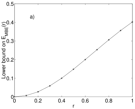
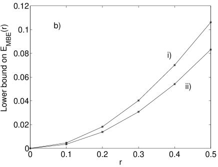
Figure 4: Plots of lower bounds on $E_{\rm MBE}$ (dimensionless) for $|\psi_{\rm CM}\rangle$ as a function of $r$ (dimensionless) for a) $N=2$ (4-way entanglement), b) (i) $N=3$ (6-way entanglement) and (ii) $N=4$ (8-way entanglement). Note that in all figures we have linearly interpolated between points 0.1 units apart on horizontal axes. Numerical errors are less than $10^{-3}$ for all data points.

As $|\psi_{\rm CM}\rangle$ is the sum of an infinite number of statevectors, to calculate $S_{L}$ in practice, we truncate the sum over ${\cal N}$ in the definition of $|\psi_{\rm CM}\rangle$ at a finite value. This induces errors in our lower bounds for $E_{\rm MBE}(|\psi_{\rm CM}\rangle)$ for which upper bounds can be derived. For all data points in Figs 4 (a) and (b), the errors on our lower bounds for $E_{\rm MBE}(|\psi_{\rm CM}\rangle)$ have been calculated to be less than $10^{-3}$ and hence are negligible.

Two interesting features of Figs 4 (a) and (b) are that, firstly, for a given $r$ value our lower bound on $E_{\rm MBE}$ decreases for increasing $N$. It is possible that we can understand this behaviour by observing that for constant $r$ we initially have a fixed entanglement resource, namely the entangled output of the NOPA. It is conceivable that the decrease under consideration results from this fixed resource being spread amongst a larger number of subsystems as we increase $N$ thus, perhaps, causing it to distribute less bipartite entanglement to any given bipartite split of $|\psi_{\rm CM}\rangle$. In turn, this may decrease the $S_{L}$ of both halves of an arbitrary split, thus explaining the decrease in our lower bound for $E_{\rm MBE}$ for increasing $N$. The second interesting feature of Figs 4 (a) and (b) is that as we increase $r$, $E_{\rm MBE}$ increases as expected given that an increased $r$ means that we have more centre-of-mass entanglement.

V Discussion

Throughout the paper, we have emphasised that $|\psi_{\rm CM}\rangle$ contains $2N$-way entanglement. However, for this entanglement to be meaningful it must have observable effects. One feature of the system under consideration that makes its entanglement conducive to producing such effect is the fact that the atoms in the system are spatially separated and thus, in principle, individually accessible. Thus, for example, we could shine a sufficiently narrow laser beam on one of the atoms and, provided it did not propagate perpendicular to the $x$-axis, implement a local displacement on the vibrational state of the atom in the $x$ direction. Furthermore, accessing individual atoms is made easier by the fact that neighbouring atoms do not have be located at successive cavity-field nodes. Instead, they can occupy every second, third etc. node, thus increasing their spatial separation and making it easier to address them one at a time. Another advantageous consequence of the fact that each atom is individually accessible is that it permits us to perform measurements on the vibrational states of single atoms, perhaps by employing a quantum-optical technique used to measure the position of individual trapped atoms by having them interact strongly with a low-photon number cavity mode hood00 .

In light of the considerations of the previous paragraph, some possible applications of the entanglement in $|\psi_{\rm CM}\rangle$ are as follows:

1. Violations of inequalities based on local realism. A number of such inequalities for an arbitrary number of quantum systems have been formulated multi_party_bell . Given the close connection between violations of these inequalities and entanglement, $|\psi_{\rm CM}\rangle$ is the sort of state we might expect to violate at least some $2N$-party inequalities based on local realism. However, as the Hilbert space for the vibrational motion each atom is infinite-dimensional and not two-dimensional as is the case for qubits, the violations may require discretising or “binning” measurement results of a continuous variable such as quadrature phase amplitude.

2. Solving quantum communication complexity problems (distributed quantum computing). Quantum communication complexity problems grover97 involve a number of parties attempting to evaluate some function $f$ for a particular input string. Each party is given part of the input string and then uses shared prior entanglement, local classical computation and public communication in attempting to evaluate $f$. In such a scenario, the prior entanglement can allow the evaluation to be performed in a superior manner to that attainable classically. As the entanglement in $|\psi\rangle_{\rm CM}$ is such that every atom in the corresponding system is with every other one, it is a quantum resource seemingly well-suited to being of use to in solving quantum communication complexity problems better than can be done classically.

3. Continuous-variable quantum computation. Continuous-variable quantum computation lloyd99 involves quantum computing with infinite-dimensional quantum systems as opposed to the usual two-dimensional qubits. The most obvious way to perform this sort of computation with the system under consideration would be to, firstly, consider each atom in it as a qudit in the limit of $d\rightarrow\infty$. After this, we would then need to implement two-qudit gates by having different atoms interact with each other in a pairwise manner. One method by which this might be accomplished is by using a scheme deutsch00 employed in optical lattices to get two spatially-separated trapped neutral atoms of different species to interact with one another. This is done by varying the polarisations of the electromagnetic fields trapping the atoms which has the effect of varying the potentials that the atoms see in such a manner that they move towards each other. Once together, the atoms interact via a dipole-dipole coupling. It is conceivable that this method could be applied to implement two-qudit gates in the system of interest. One complication, however, in utilising this scheme is that it necessitates that we modify our system by having the $2N$ atoms in it comprised of two different species, perhaps with the species of atom alternating as we move along each linear configuration. Nevertheless, whilst the system under consideration may not be the most natural one in which to do continuous-variable quantum computation, there is some possibility that the entanglement in it could be used to do this.

V.1 Qualitative results

The thinking underlying Definition 1 is the same as that which underlies the NPT sufficient condition for $M$-way entanglement. However, there are significant differences between the two. Firstly, Definition 1 involves arbitrary dimensional subsystems, whereas the NPT sufficient condition deals only with qubits. Secondly, the NPT sufficient condition is a sufficient but not a necessary condition for $M$-way entanglement whereas the satisfaction of Definition 1 is both necessary and sufficient for pure states. Thirdly, the NPT sufficient condition uses the partial transpose to determine the presence of $M$-way entanglement, whereas Definition 1 uses the mathematically simpler entity the trace of the square of a reduced density operator. Observe that Definition 1 is narrower than the NPT sufficient condition in the sense that it only applies to pure states whilst the NPT sufficient condition is applicable to both pure and mixed states.

V.2 Quantitative results

A number of issues surround $E_{\rm MBE}$, which we now discuss.

1. What does $E_{\rm MBE}$ tell us about what quantum resource we have? Ideally, we would like to be able to relate $E_{\rm MBE}$ to one or more quantum tasks or protocols such as distributed quantum computation with $E_{\rm MBE}$ telling us something valuable about how well we can perform these tasks. This is so as if we could do this, then it would increase $E_{\rm MBE}$’s utility. Unfortunately, however, this has not yet been accomplished.

2. Can we tractably calculate $E_{\rm MBE}$? For an entanglement measure to be useful, it must be tractable and able to be calculated in practice. Unfortunately, $E_{\rm MBE}$ seems to be difficult to calculate, at least for the state considered.

Although $E_{\rm MBE}$ has the two above negative features we note that, firstly, further research may eliminate them and, secondly, we should consider them alongside the positive features of $E_{\rm MBE}$ which are that it is a reasonable measure and that it helps us to understand the nature of the entanglement in $|\psi_{\rm CM}\rangle$ and also the capabilities of quantum state exchange. Our results contribute to the understanding of multipartite entanglement involving massive particles and infinite-dimensional Hilbert spaces within a context that is not overly experimentally infeasible.

To conclude, we have shown that quantum state exchange can be used to produce the state $|\psi_{\rm CM}\rangle$ for two sets of trapped atoms in spatially separated FORTs. We have also show that $|\psi_{\rm CM}\rangle$ is a $2N$-way entangled state and, in addition, have placed a lower bound on the amount of such entanglement that it possesses. Finally, we have discussed quantum information processing tasks that the $2N$-way entanglement in $|\psi_{\rm CM}\rangle$ could be used to help perform.

VI Acknowledgements

DTP would like to thank Drs Scott Parkins, Bill Munro, Tobias Osborne and Tim Ralph for valuable discussions. He would also like to thank the referee for highlighting a shortcoming in the orginal version and, finally, Dr Derrick Siu.

References

- (1) R. Jozsa and N. Linden, arXive e-print quant-ph/0201143.
- (2) M. A Nielsen and I. L. Chuang, Quantum Computation and Quantum Information (Cambridge University Press, Cambridge, 2000).
- (3) J. Preskill, Physics 229: Advanced Mathematical Methods of Physics — Quantum Computation and Information. California Institute of Technology, 1998. URL: http://www.theory.caltech.edu/people/preskill/ph229/
- (4) M. Żukowski and D. Kaszlikowski, Phys. Rev. A 59, 3200 (1999).
- (5) J. Preskill, J. Mod. Optics 47,127 (2000).
- (6) V. Vedral, M. B. Plenio, M. A. Rippen, and P. L. Knight, Phys. Rev. Lett. 78, 2275 (1997).
- (7) V. Coffman, J. Kundu, and W. Wootters, Phys.Rev. A61 (2000) 052306.
- (8) W. K. Wootters, Phys. Rev. Lett. 80, 2245 (1998).
- (9) G. Vidal, J. Mod. Opt. 47, 355 (2000).
- (10) D. A. Meyer and N. R. Wallach, arXive e-print quant-ph/0108104.
- (11) A. Wong and N. Christensen, Phys. Rev. A 63, 044301 (2001).
- (12) O. Biham, M. A. Nielsen, and T. J. Osborne, arXive e-print quant-ph/0112097.
- (13) L. Grover, Phys. Rev. Lett. 79, 325 (1997).
- (14) A. S. Parkins and H.J. Kimble, J. Opt. B: Quantum Semiclass. Opt. 1 496 (1999).
- (15) A. S. Parkins and H. J. Kimble, Phys. Rev. A 61, 052104 (2000).
- (16) A.S. Parkins and H.J. Kimble, arXive e-print quant-ph/9909021.
- (17) A. S. Parkins, J. Opt. B: Quantum Semiclass. Opt. 3, S18 (2001).
- (18) A. S. Parkins and E. Larsabal, Phys. Rev. A 63, 012304 (2001).
- (19) Z. Y. Ou, S. F. Pereira, H. J. Kimble, and K. C. Peng, Phys. Rev. Lett. 68, 3663 (1992).
- (20) Z. Y. Ou, S. F. Pereira, and H. J. Kimble, Photophys. Laser Chem. 55, 265 (1992).
- (21) H. J. Kimble, in Fundamental Systems in Quantum Optics, Proceedings of the Les Houches Summer School of Theoretical Physics, Session LIII, Les Houches, 1990, edited by J. Dalibard et al. (Elsevier, New York, 1992).
- (22) J. D. Miller, R. A. Cline, and D. J. Heinzen, Phys. Rev. A 47, R4567 (1993).
- (23) H. J. Lee et al., Phys. Rev. Lett. 76, 2658 (1996).
- (24) P. S. Jesson and I. H. Deutsch, Adv. Atom. Mol. Opt. Phys. 37, 415 (1996).
- (25) D. L. Haycock et al., Phys. Rev. A 55, R3991 (1997).
- (26) I. Deutsch, Phys. Rev. A 57, 1972 (1998).
- (27) See, for example, M. G. Raizen et al., Phys. Rev. A 45, 6493 (1992), H. Walther, Adv. At. Mod. Opt. Phys. 32, 379 (1994) and D. J. Wineland et al., J. Res. Natl Inst. Stan. 103, 259 (1998).
- (28) A. B. Mundt et al., unpublished, arXiv:quant-ph/0202112.
- (29) S. Van Enk, J. McKeever, H.J. Kimble, and J. Ye, Phys. Rev. A 64, 013407 (2001).
- (30) W. Dür and I. Cirac, Phys. Rev. A 61, 042314 (2000).
- (31) A. Peres, Phys. Lett. A 77, 1413 (1996).
- (32) M. Horodecki, P. Horodecki, and R. Horodecki, Phys. Lett. A 223, 8 (1996).
- (33) M. Horodecki, P. Horodecki, and R. Horodecki, Phys. Rev. Lett. 78, 574 (1997).
- (34) A. Peres, Quantum theory: concepts and methods (Kluwer Academic, Dordrecht, 1993)
- (35) D. A. Rice, C. F. Osborne, and P. Lloyd, Phys. Lett. A 186, 21 (1994).
- (36) M. B. Plenio and V. Vedral, Contemp. Phys. 39, 431 (1998).
- (37) S. Bose and V. Vedral, Phys. Rev. A 61, 040101 (2000).
- (38) For example N. D. Mermin Phys. Rev. Lett. 65, 1838 (1990); M. Ardenhali, Phys. Rev. A 46, 5375 (1992); A. V. Belinskii and D. N. Klyshko, Phys. Ups. 36, 653 (1993); M. Zukowski and C. Brukner Phys. Rev. Lett. 88, 210401 (2002).
- (39) L. K. Grover, quant-ph/9704012.
- (40) C. J. Hood et al. Science 287, 1447 (2000).
- (41) S. Lloyd and S. L. Braunstein, Phys. Rev. Lett. 82, 1784 (1999).
- (42) I. H. Deutsch, G. K. Brennen, and P. S. Jessen Fort. der Phys. 48, 925 (2000).