Simple optical measurement of the overlap and fidelity of quantum states: An experiment

Abstract

We present the experimental results of measurements of the overlap of both pure and mixed polarization states of photons. The fidelity and purity of mixed states were also measured. The experimental apparatus exploits the fact that a beam splitter can distinguish the singlet Bell state from the other Bell states, i.e., it realizes projections into the symmetric and antisymmetric subspaces of photons’ Hilbert space.

Recently it was theoretically shown by several authors that many important characteristics of quantum states such as the purity, overlap, and fidelity can be measured directly radim ; ek-hor without carrying out a complete quantum-state reconstruction. However, the proposed experimental setups were rather complicated. They involved cavity QED, non-linear optics, etc. The only reported experimental test is based on NMR Fei02 . In this Letter we show that for two qubits, encoded into the polarization states of photons, the same goal can be achieved with a simple beam splitter. Besides, the same setup with a beam splitter can serve as the recently proposed FiDuFi universal measurement device programmed by a quantum state (where the polarization of one photon is measured, while the polarization state of the other photon serves as the “program”).

Let us consider a flip operator $V$ in the Hilbert space $\mathcal{H}\otimes\mathcal{H}$ of two distinguishable but equivalent subsystems: $V\,|\psi\rangle\otimes|\phi\rangle=|\phi\rangle\otimes|\psi\rangle$. Let us further consider a factorable state $\rho_{\mathrm{A}}\otimes\rho_{\mathrm{B}}$ in the same Hilbert space. Then it follows from a direct calculation that ${\mathrm{Tr}}(V\rho_{\mathrm{A}}\otimes\rho_{\mathrm{B}})={\mathrm{Tr}}(\rho_{\mathrm{A}}\rho_{\mathrm{B}})\equiv F$; note that $\rho_{\mathrm{A}}\rho_{\mathrm{B}}$ is not a direct product. Taking into account the relation $V=\Pi^{+}-\Pi^{-}$, where $\Pi^{+}$ and $\Pi^{-}$ are projectors to the symmetric and antisymmetric subspaces of $\mathcal{H}\otimes\mathcal{H}$, respectively, one finally obtains

$${\mathrm{Tr}}\left(\rho_{\rm A}\rho_{\rm B}\right)={\mathrm{Tr}}\left(\Pi^{+}\rho_{\rm A}\otimes\rho_{\rm B}\right)-{\mathrm{Tr}}\left(\Pi^{-}\rho_{\rm A}\otimes\rho_{\rm B}\right).$$ (1)

It means that if we were able to implement projections to the symmetric and antisymmetric subspaces we could measure the overlap of two general states living in $\mathcal{H}$. In particular, we would be able to measure the overlap of two pure states, $|\langle\psi|\phi\rangle|^{2}$, the fidelity $\langle\psi|\rho|\psi\rangle$ comparing the state $\rho$ with the “original” state $|\psi\rangle$, and also to calculate the Hilbert-Schmidt distance of two general states:

$$d(\rho_{\mathrm{A}},\rho_{\mathrm{B}})=\left[\frac{1}{2}{\mathrm{Tr}}\,(\rho_{\mathrm{A}}-\rho_{\mathrm{B}})^{2}\right]^{1/2}.$$ (2)

Besides, having a device realizing projective measurement $\{\Pi^{+},\Pi^{-}\}$, we could experimentally implement the simplest version of a quantum “multimeter” controlled by quantum “software” that has been proposed in Ref. FiDuFi . In this concept, one qubit (the “program”) determines the measurement basis for a projective measurement on the other qubit. Of course, any such measurement can be realized only approximately (with some error-rate). It has been shown FiDuFi that under given conditions, the optimal multimeter that maximizes the average fidelity is represented by a projective measurement on the “program” and “data” together. This measurement is described exactly by projectors to the symmetric and antisymmetric subspaces of the “program-data” Hilbert space.

Now let us turn our attention to the polarization states of two photons. The states corresponding to the horizontal and vertical linear polarizations will be denoted as $|{H}\rangle$ and $|{V}\rangle$, respectively. In such a case the projector into the antisymmetric subspace has the following form $\Pi^{-}=|\Psi^{-}\rangle\!\langle\Psi^{-}|$, where

$$|\Psi^{-}\rangle=\frac{1}{\sqrt{2}}\Bigl{(}|{H}\rangle_{1}|{V}\rangle_{2}-|{V}\rangle_{1}|{H}\rangle_{2}\Bigr{)}$$ (3)

is nothing else but a singlet state BCJ . What happens if a singlet impinges on a beam splitter? It is an elementary exercise to show that a beam splitter transforms it to the state $(|{H}\rangle_{3}|{V}\rangle_{4}-|{V}\rangle_{3}|{H}\rangle_{4})/\sqrt{2}$ (the labeling of the inputs and outputs of the beam splitter is shown in Fig. 1). Such a state results in a simultaneous detection at both detectors placed in modes 3 and 4 Weinfurter94 ; Braunstein95 ; innsbruck ; Mattle96 ; Bouwmeester97 . The singlet is the only one of the four Bell states (completing the basis in the Hilbert space of two qubits) that produces such a coincidence detection. The other Bell states make only one of the detectors fire. This fact makes the measurement on two qubits consisting of projectors $\Pi^{+}$ and $\Pi^{-}$ experimentally feasible. The beam splitter can be seen as a universal quantum device suitable for the experimental realization of all the tasks discussed above.

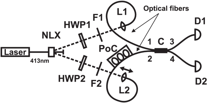
Figure 1: Setup of the experiment. NLX – nonlinear crystal, HWP – half-wave plates, F – long-wave pass filters (cut-off at 670 nm), L – lenses, PoC – polarization controller, C – fiber coupler, D – detectors.

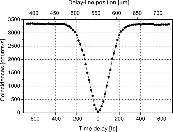
Figure 2: Hong-Ou-Mandel dip.

The experimental setup is shown in Fig. 1. A Kr⁺-ion laser of wavelength 413.1  nm illuminates a 10-mm-long nonlinear crystal of LiIO₃ (cut $\theta=90^{\circ},\phi=0^{\circ}$), where spontaneous parametric non-collinear degenerate type-I down-conversion occurs. After passing through the respective half-wave plates (HWP), the down-converted photons are coupled into optical fibers and combined at a fused 50/50 fiber coupler, thus forming a Hong-Ou-Mandel interferometer Mandel . Since optical fiber deforms polarization states, one of the arms of the interferometer contains a polarization controller to match the polarizations of signal and idler beams at the coupler. The polarization controller consists of several loops of fiber acting as a set of a half-wave plate and two quarter-wave plates. Single-photon counting modules (employing silicon avalanche photodiodes with quantum efficiency $\eta=51\%$) are placed at the output ports of the coupler and electronics measure their coincidence rate. With this setup, visibilities exceeding 98 % were reached. Higher visibilities could not be reached due to the fact that the splitting ratio of the fiber coupler was not exactly 50/50 and due to the imperfections of the half-wave plates. A typical Hong-Ou-Mandel dip is shown in Fig. 2. Different time delays were generated by moving the coupling lens L2 and the tip of the fiber towards the nonlinear crystal. Moving the coupling stage $200\,{\mu}$m away from the center of the dip also served to measure the coincidence rate $C_{200}$ on the shoulder for normalization purposes (it represents a half of the impinging-pair rate). According to Eq. (1) the overlap is calculated from measured data as follows:

$${\mathrm{Tr}}(\rho_{A}\rho_{B})=1-2{\mathrm{Tr}}(\Pi^{-}\rho_{A}\otimes\rho_{B})=1-\frac{C_{0}}{C_{200}},$$ (4)

where $C_{0}$ is a coincidence rate when the arms of the interferometer are balanced.

Each data point at presented plots has been derived from 50–200 one-second measurement periods. On average, 3300 coincidences per second were measured on the shoulder away from the dip. Statistical errors are smaller than the symbols of points in the graphs. Other errors stem from the non-unit visibility and optical-path fluctuations. The accuracy of polarization-angle settings was better than $\pm 0.3^{\circ}$.

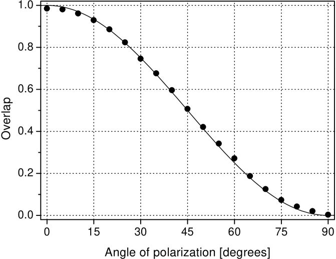
Figure 3: Overlap of two pure states. The first photon is in the state with vertical linear polarization ($\theta=0$). The other photon is also linearly polarized but its polarization is rotated by angle $\theta>0$.

The main results of this Letter are shown in Figs. 3–6. First we measured the overlap of two pure states. Generated downconverted photon pairs were linearly polarized in the vertical direction. The polarization of photons in Arm 1 was kept fixed and the polarization angle $\theta$ of photons in Arm 2 was varied by rotating the half-wave plate HWP2. Thus we measured the overlap between the states $|V\rangle$ and $\cos\theta\,|V\rangle+\sin\theta\,|H\rangle$. The experimental results shown in Fig. 3 are in very good agreement with the theoretically expected dependence $\cos^{2}\theta$ that is also plotted in Fig. 3.

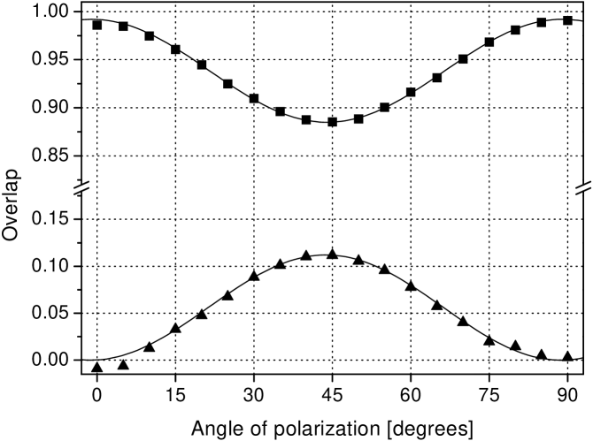
Figure 4: Overlap of two pure states (5) with $\vartheta=\theta$ (squares) and $\vartheta=\theta+\pi/2$ (triangles); $\vartheta$ is the polarization angle of the photon in Arm 1, $\vartheta$ is the polarization angle of the photon in Arm 2.

In the next round of the measurements we simultaneously changed the polarization states of both photons by rotating both half-wave plates. In the first arrangement, both photons were linearly polarized in the same direction $\theta$ after passing through the half-wave plates and one would expect the overlap to be equal to one for all $\theta$. In the second arrangement the two photons were linearly polarized in perpendicular directions, hence their polarization states were orthogonal and the theory predicts $F=0$ for all $\theta$.

However, a different behavior was observed – see Fig. 4. The dependence of the overlap on angle $\theta$ can be explained by the modification of the polarization state inside the fibers due to birefringence and other effects. This effect must be compensated for by the polarization controller whose proper setting should ensure that if the two photons enter the fibers in the identical polarization states, then they also arrive at the fiber coupler in identical polarization states. It is relatively easy to satisfy this condition for some chosen basis states, say $|H\rangle$ and $|V\rangle$, for which the visibility of the dip is tuned to maximum by manipulating the polarization controllers; however, this does not guarantee that the above condition will be satisfied for any polarization state. What happens in the fibers is that the horizontally polarized photon acquires certain non-zero phase shift with respect to the vertically polarized one. This shift is different, in general, for the fiber in Arm 1 and Arm 2. Therefore, the polarization of the two photons at the coupler is not the same even if the input polarization states are identical. However, this phase shift does not play any role if at least one of the photons is in the basis state $|H\rangle$ or $|V\rangle$. Due to the technical difficulties with the fiber polarization controller, we were not able to compensate for such phase shifts. The phenomenon can be described by an effective phase shift $\phi$ of one of the input polarization states. In our setup, we thus effectively prepare the following polarization states of photons,

$$|\psi_{1}\rangle = e^{i\phi}\cos\theta\,|V\rangle+\sin\theta\,|H\rangle,$$

$$|\psi_{2}\rangle = \cos\vartheta\,|V\rangle+\sin\vartheta\,|H\rangle,$$ (5)

where $\theta$ and $\vartheta$ are controlled by rotating the half-wave plates, and the fixed phase shift $\phi$ is a parameter of our apparatus. The outcomes of measurements with $\vartheta=\theta$ and $\vartheta=\theta+\pi/2$ are shown in Fig. 4. The formulas for the overlaps read:

$$F_{||} = 1-\sin^{2}(2\theta)\sin^{2}(\phi/2),$$

$$F_{\perp} = \sin^{2}(2\theta)\sin^{2}(\phi/2).$$ (6)

The solid lines in Fig. 4 display the best fits of the form $A+B\sin^{2}(2\theta)$, with $A_{\perp}=0$, $B_{\perp}=0.112$, $A_{||}=0.992$, and $B_{||}=0.107$. A very good agreement between the theory (6) and experimental data is observed. From the fit we can extract the absolute value of the phase shift, $|\phi|=39.4^{\circ}\pm 0.3^{\circ}$. In the future experiment, we plan to insert a Pockels cell between the half-wave plate HWP1 and the fiber which will allow us to compensate for the phase shift $\phi$ and vary it at will.

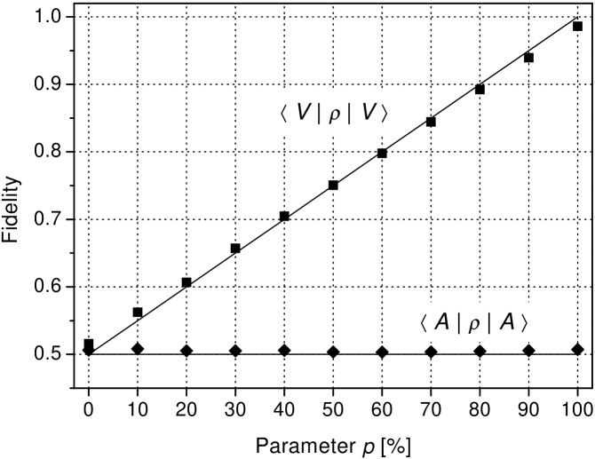
Figure 5: Measurement of the fidelity of a mixed state with respect to two different pure states $|V\rangle$ and $|A\rangle$. The full lines represent theoretical values.

So far we have focused on the overlap of two pure states. Our device can also be used to measure the fidelity of a mixed state with respect to a pure state or the overlap of two mixed states. The mixed state $\rho$ was created as a mixture of three pure states $|V\rangle$, $|X\rangle$ and $|Y\rangle$,

$$\rho=p\,|V\rangle\langle V|+\frac{1-p}{2}(|X\rangle\langle X|+|Y\rangle\langle Y|),$$ (7)

where $|X\rangle$ and $|Y\rangle$ stand for two mutually orthogonal polarization states. In the experiment, states $|X\rangle$ and $|Y\rangle$ were generated by setting $\theta=45^{\circ}$ and $\theta=-45^{\circ}$, respectively. The measured dependence of the fidelity $F=\langle\psi|\rho|\psi\rangle$ on the parameter $p$ is shown in Fig. 5 for two different pure states $|V\rangle$ and $|A\rangle=(|V\rangle+|H\rangle)/\sqrt{2}$.

Let us now turn our attention to the overlap of two mixed states. A particularly interesting case occurs if $\rho_{\rm A}=\rho_{\rm B}=\rho$ because the overlap is then equal to the purity of $\rho$, ${\rm Tr}(\rho_{\rm A}\rho_{\rm B})={\rm Tr}(\rho^{2})$. To demonstrate this, we prepared both photons in the same mixed state (7) following the procedure described above. The measured purity is plotted in Fig. 6 as a function of $p$. If we know the purity $P$ of the qubit state $\rho$, we can immediately determine the eigenvalues of $\rho$ from the formula

$$\lambda_{1,2}=\frac{1}{2}(1\pm\sqrt{2P-1}).$$ (8)

Our experimental setup thus enables a direct estimation of the eigenvalues of $\rho$ without the necessity to reconstruct the whole density matrix provided that two copies of $\rho$ are available simultaneously for a joint measurement on $\rho\otimes\rho$. The obtained eigenvalues are plotted in Fig. 6. They are in good agreement with the theoretically expected behavior. The largest errors of eigenvalues occur when $\rho$ is close to the maximally mixed state where $P\approx 1/2$ and a small error in $P$ causes a large error in $\lambda$ as can be deduced from Eq. (8). Note also that if we know the spectrum of $\rho$, then we can determine several important characteristics of $\rho$ such as the von Neumann entropy ${\rm Tr}(\rho\ln\rho)=\sum_{j=1}^{2}\lambda_{j}\ln\lambda_{j}$.

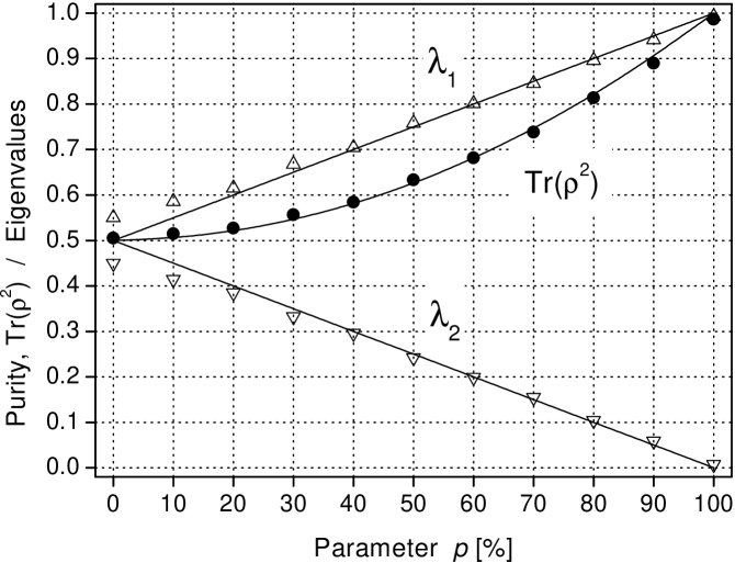
Figure 6: Measurement of the purity of mixed state (7) – circles. The full line represents the theoretical prediction $P=(1+p^{2})/2$. The triangles denote the eigenvalues of corresponding density matrices, calculated from the purity.

Table 1: Measured overlap $F$ and Hilbert-Schmidt distance $d$ of two mixed states. The columns labeled by $F_{\rm th}$ and $d_{\rm th}$ show the theoretical values for comparison.

$p_{\rm A}$	$p_{\rm B}$	$F$	$F_{\rm th}$	$d$	$d_{\rm th}$
0.2	0.4	0.545	0.540	0.097	0.100
0.2	0.6	0.563	0.560	0.197	0.200
0.2	0.8	0.581	0.580	0.298	0.300
0.4	0.6	0.621	0.620	0.096	0.100
0.4	0.8	0.658	0.660	0.201	0.200
0.6	0.8	0.736	0.740	0.099	0.100

Finally, we experimentally determined the overlap of two different mixed states $\rho_{\rm A}$ and $\rho_{\rm B}$ of the form (7). The results for several different parameters $p_{\rm A}$ and $p_{\rm B}$ are summarized in Table 1. If we combine these data with the direct measurement of the purity of states $\rho_{\rm A}$ and $\rho_{\rm B}$, we can calculate the Hilbert-Schmidt distance $d(\rho_{\rm A},\rho_{\rm B})$ from Eq. (2) – the results are also shown in Table 1.

As mentioned in the introduction, our experimental device can also serve as a “quantum multimeter” FiDuFi . The polarization state of one input photon, $|\psi\rangle$, represents a program (it determines the measurement basis spanned by $|\psi\rangle$ and its orthogonal counterpart $|\psi_{\perp}\rangle$). The other input photon represents the measured qubit (in some “unknown” state $|\varphi\rangle$). A coincident detection corresponds to the measurement result “one”, a detection at only one of the detectors corresponds to the measurement result “two”. The probabilities of the results “one” and “two”, respectively, read: $p_{\perp,||}(\psi,\varphi)=\left[1\mp|\langle\psi|\varphi\rangle|^{2}\right]/2$. Of course, in reality the performance of the multimeter is impaired by the low detection efficiency. Nevertheless, we can still verify the predicted fidelity of such a multimeter. It is given by the formula FiDuFi :

$$F(\psi)=\frac{1}{2}\left[p_{||}(\psi,\psi)+p_{\perp}(\psi,\psi_{\perp})\right].$$ (9)

As we can measure the overlaps, we can also determine this function. For the three program states of the form $\cos\theta\,|V\rangle+\sin\theta\,|H\rangle$, the corresponding fidelities are shown in the following table: $\theta$: $0^{\circ}$ $-45^{\circ}$ $45^{\circ}$ $F$: 0.742 0.748 0.748 The deviation from the theoretical value $3/4$ is mainly due to the non-unit visibility.

- (1) R. Filip, Phys. Rev. A 65, 062320 (2002).
- (2) A. K. Ekert et al., Phys. Rev. Lett. 88, 217901 (2002).
- (3) X. Fei, D. Jiangfeng, W. Jihui, Z. Xianyi, and H. Rongdian, quant-ph/0204049.
- (4) J. Fiurášek, M. Dušek and R. Filip, quant-ph/0202152.
- (5) S. M. Barnett, A. Chefles, and I. Jex, quant-ph/0202087.
- (6) H. Weinfurter, Europhys. Lett. 25, 559 (1994).
- (7) S. L. Braunstein and A. Mann, Phys. Rev. A 51, R1727 (1995).
- (8) M. Michler, K. Mattle, H. Weinfurter, and A. Zeilinger, Phys. Rev. A 53, R1209 (1996).
- (9) K. Mattle, H. Weinfurter, P. G. Kwiat, and A. Zeilinger, Phys. Rev. Lett. 76, 4656 (1996);
- (10) D. Bouwmeester, J. W. Pan, K. Mattle, M. Eibl, H. Weinfurter, and A. Zeilinger, Nature (London) 390, 575 (1997).
- (11) C. K. Hong, Z. Y. Ou, and L. Mandel, Phys. Rev. Lett. 59, 2044 (1987).