Quantum dynamics as a physical resource

Abstract

How useful is a quantum dynamical operation for quantum information processing? Motivated by this question we investigate several strength measures quantifying the resources intrinsic to a quantum operation. We develop a general theory of such strength measures, based on axiomatic considerations independent of state-based resources. The power of this theory is demonstrated with applications to quantum communication complexity, quantum computational complexity, and entanglement generation by unitary operations.

I Introduction

The quantification and comparison of different types of physical resources lies at the heart of much of modern science. A good example is the physical resource energy, whose quantification enabled the development of thermodynamics. More recently, motivated by applications to quantum information processing, there have been attempts to develop a quantitative theory of quantum entanglement Bennett et al. (1996). This theory, still in its nascent stages, has been applied to gain insight into questions about the capacity of a noisy channel for information Schumacher and Westmoreland (2002), quantum teleportation with a noisy entangled resource Horodecki et al. (1999), and distributed quantum computation Nielsen (1998).

Structurally, quantum mechanics has two parts, one part concerned with quantum states, the other with quantum dynamics. A general quantum dynamical process is described by a quantum operation (reviewed in Nielsen and Chuang (2000)); such processes include unitary evolution, quantum measurement, dissipation, and decoherence. We believe quantum operations are a useful physical resource on an equal and logically independent footing to quantum states.

The first step in studying a physical resource is to quantify it. Therefore, the purpose of our paper is to develop a theory quantifying the strength of quantum dynamical operations. Our motivations are axiomatic and operational questions concerning quantum dynamics. Our goal is to find strength measures capturing some of the structure in the complicated space of quantum operations, to gain insight into quantum dynamics and complex quantum systems Nielsen (2002); Osborne (2002). Although some of the measures we propose for operations are based on state entanglement measures, we expect the study of dynamics to provide different, complementary insights to those gained from the study of states.

What questions will good strength measures allow us to analyze? We foresee applications to the analysis of quantum computational complexity, distributed quantum computation, quantum communication, and quantum cryptography. As a simple example, consider the question of how many controlled-not (cnot) gates are required to implement a swap gate on two qubits, when assisted by arbitrary local unitaries. Suppose we have a measure $K(U)$, quantifying the strength of a unitary $U$. Suppose further that $K(U)$ satisfies (a) $K(UV)\leq K(U)+K(V)$; and (b) $K(U)=0$ for local unitaries $U$. It is easy to see that the number of cnot gates needed to do the swap gate is at least $K(\textsc{swap})/K(\textsc{cnot})$.

More generally, the central problem of quantum computational complexity is to determine the minimum number of one- and two-qubit gates necessary to implement a desired $n$-qubit unitary operation $U$. For example, $U$ might encode the solution to a problem such as the traveling salesman problem. Suppose we have a strength measure satisfying properties (a) and (b), above, as well as (c) $K(U\otimes I)=K(U)$. The number of gates needed to compute $U$ is again bounded below by $K(U)/K(\textsc{cnot})$. Such a bound might help in determining the relationships between various quantum and classical complexity classes. We will return to this application several times.

Another motivation to study quantum dynamics as a resource is recent work on universality in quantum computation. The class of interactions capable of performing universal quantum computation has been shown to be the class of bipartite entangling dynamics; any Hamiltonian which can create entanglement between any pair of qudits is universal, when assisted by arbitrary one-qudit unitaries (see Dodd et al. (2002); Wocjan et al. (2002); Dür et al. (2001); Bennett et al. (2001); Nielsen et al. (2001); Vidal et al. (2002a) and references therein, see also Jones and Knill (1999); Leung et al. (2000) for related work). It has also been shown that any entangling two-qudit unitary, together with arbitrary one-qudit unitaries, is universal (Brylinski and Brylinski (2002), see Bremner et al. (2002) for a simple, constructive proof in the qubit case).

These results show that there is a qualitative difference between entangling and non-entangling dynamics. Furthermore, they show all two-qudit entangling dynamics are qualitatively equivalent, as any one can simulate any other, provided local unitaries are available. By analogy with the study of state entanglement, this suggests quantifying entangling dynamics. We now review prior work on this idea, organizing our discussion around three motivating themes: the communication cost to implement an operation; the entangling ability of an operation; and the ability of an operation to communicate bits.

The communication requirements for implementing a general bipartite unitary $U$ were studied in Ch. 6 of Nielsen (1998), where a general lower bound on the number of qubits of communication needed to implement $U$ was proved, depending only on the operator Schmidt decomposition of $U$ (see Sec. II for discussion of this decomposition). Eisert et al. Eisert et al. (2000) and Collins, Linden, and Popescu Collins et al. (2001) studied the classical communication and entanglement required to implement some specific few-qubit quantum gates. Chefles, Gilson, and Barnett Chefles et al. (2001) studied the amount of communication and entanglement required to perform an arbitrary gate in a network of qubits.

The capacity of a quantum operation to generate entanglement seems to have first been studied by Makhlin Makhlin (2000), who found three invariants characterizing the non-local properties of two-qubit unitaries. Makhlin used the invariants to obtain results about entanglement generation, with a view towards applying them to the complexity of implementing gates. Zanardi, Zalka, and Faoro Zanardi et al. (2000), Zanardi Zanardi (2001), and Wang and Zanardi Wang and Zanardi (2002), all obtained results about the average entanglement generated by a unitary. Cirac et al. Cirac et al. (2000) studied the ability of an operation to produce entanglement by mapping the operation onto a corresponding state, and studying the properties of that state. Kraus and Cirac Kraus and Cirac (2001) studied the maximum entanglement which can be created by a unitary operator acting on two initially unentangled qubits. They found an explicit formula for the maximum entanglement that can be generated without ancillas, and showed that this amount can be exceeded with the use of ancillas. Leifer, Henderson, and Linden Leifer et al. (2002) used similar reasoning to obtain an explicit formula for the entanglement generated without ancillas, but allowing initial entanglement. They also obtained numerical results demonstrating that the addition of ancillas can increase the maximum entanglement generated. In a different context, Scarani et al Scarani et al. (2002) related the entangling power of a unitary operation to the problem of thermalization of a quantum system.

A related approach is to quantify the entangling abilities of Hamiltonians rather than unitaries. Dür et al. Dür et al. (2001) considered the rate at which a Hamiltonian creates entanglement, and found techniques to optimize this rate. More recently, Vidal, Hammerer, and Cirac Vidal et al. (2002b) (see also Hammerer et al. (2002)) analytically characterized the minimum time required to simulate one Hamiltonian with another, and found the minimum time required to simulate a desired unitary with a Hamiltonian. This allowed them to define a partial order on unitaries, according to which one unitary $U$ is more non-local than another unitary $V$ if and only if, for any Hamiltonian, the minimum time required to simulate $U$ is longer than the minimum time to simulate $V$. They also obtained results on the optimal choices of non-local interactions for transmitting classical bits between two parties. Childs et al. Childs et al. (2002) found an explicit formula for the maximum entanglement created by a class of two-qubit Hamiltonians, including the Ising interaction and the anisotropic Heisenberg interaction, for which this maximum is achieved without ancillas.

The ability of a quantum operation to communicate classical information was studied by Beckman et al. Beckman et al. (2001), who obtained simple necessary and sufficient conditions for information transmission to be possible. Bennett et al. Bennett et al. (2002) and Berry and Sanders Berry and Sanders (2002) studied the capacity of a bipartite operation to communicate information, and related this capacity to the ability of the operation to generate entanglement.

Our paper draws on all these perspectives, but differs in an important way. Rather than focusing on the ability of a quantum dynamical operation to generate some static resource, such as entanglement or shared classical bits, we believe it is possible to quantify quantum dynamical operations as a physical resource in their own right. That is, we do not need to make reference to the ability of the operation to generate some other resource.

How can one develop a theory of dynamic strength without relying on familiar state-based resources? The approach we take is to identify plausible axioms and properties a good measure of strength should satisfy, and develop measures satisfying those properties.

The paper is structured as follows. Sec. II opens by introducing two concrete examples of strength measures for unitary operations, the Hartley and Schmidt strengths. Sec. III considers operational questions motivating strength measures, and uses these questions to motivate some abstract axioms for such measures. Sec. IV briefly summarizes a useful canonical decomposition for two-qubit unitary operators. Secs. V and VI explore a variety of specific definitions for dynamic strength measures. Our general philosophy is to explore a wide variety of measures, and then to concentrate on those which appear most likely to yield useful practical answers to interesting operational questions. Sec. VII concludes with a summary and a table of results.

II Invitation: the Hartley and Schmidt strengths

In this section we introduce two strength measures, the Hartley strength and the Schmidt strength. These measures are introduced both because of their intrinsic interest, and also because the Hartley strength will be used as a simple, concrete example illustrating the more abstract, axiomatic approach to dynamic strength. The Hartley and Schmidt strengths are based on a generalization of the Schmidt decomposition to operators, which we call the operator-Schmidt decomposition Nielsen (1998). To explain the operator-Schmidt decomposition we introduce the Hilbert-Schmidt inner product on the space of $d\times d$ operators, defined by $(Q,P)\equiv\mathrm{tr}(Q^{\dagger}P)$, for any operators $Q$ and $P$. Using this inner product, we define an orthonormal operator basis to be a set $\{Q_{j}\}$ which satisfies the condition: $(Q_{j},Q_{k})=\mathrm{tr}(Q_{j}^{\dagger}Q_{k})=\delta_{jk}$ where $\delta_{jk}=1$ if $j=k$ and 0 otherwise. For example, a complete orthonormal basis for the space of one-qubit operators is the set of normalized Pauli matrices, $\{\tilde{I},\tilde{X},\tilde{Y},\tilde{Z}\}\equiv\{I/\sqrt{2},X/\sqrt{2},Y/\sqrt{2},Z/\sqrt{2}\}$.

An operator $Q$ acting on systems ${\cal A}$ and ${\cal B}$ may be written in the operator-Schmidt decomposition Nielsen (1998):

$$Q=\sum\nolimits_{l}s_{l}A_{l}\otimes B_{l},$$ (1)

where $s_{l}\geq 0$ and $A_{l}$ and $B_{l}$ are orthonormal operator bases for ${\cal A}$ and ${\cal B}$, respectively. To prove the operator-Schmidt decomposition, expand $Q=\sum_{jk}M_{jk}C_{j}\otimes D_{k}$, where $C_{j}$ and $D_{k}$ are fixed orthonormal operator bases for ${\cal A}$ and ${\cal B}$, respectively, and $M_{jk}$ are coefficients. The singular value decomposition states that the matrix $M$, whose $(j,k)$th entry is $M_{jk}$, may be written $M=UsV$, where $U$ and $V$ are unitary, and $s$ is diagonal with non-negative entries. We thus obtain

$$Q=\sum_{jkl}U_{jl}s_{l}V_{lk}C_{j}\otimes D_{k},$$ (2)

where $s_{l}$ is the $l$th diagonal entry of $s$. Defining $A_{l}\equiv\sum_{j}U_{jl}C_{j}$ and $B_{l}\equiv\sum_{k}V_{lk}D_{k}$, which are easily shown to be orthonormal operator bases for ${\cal A}$ and ${\cal B}$, we obtain the operator-Schmidt decomposition Eq. (1).

Nielsen Nielsen (1998) defines the Schmidt number of an operator, $\mathrm{Sch}(Q)$, to be the number of non-zero coefficients in the operator-Schmidt decomposition for $Q$ .

A simple example is the cnot gate which has operator-Schmidt decomposition

$$\textsc{cnot}=\sqrt{2}\,|0\rangle\langle 0|\otimes\tilde{I}+\sqrt{2}\,|1\rangle\langle 1|\otimes\tilde{X}$$ (3)

and hence has Schmidt coefficients $\{\sqrt{2},\sqrt{2}\}$, and $\mathrm{Sch}(\textsc{cnot})=2$. The swap gate for qubits has operator-Schmidt decomposition

$$\textsc{swap}=\tilde{I}\otimes\tilde{I}+\tilde{X}\otimes\tilde{X}+\tilde{Y}\otimes\tilde{Y}+\tilde{Z}\otimes\tilde{Z}$$ (4)

and hence $\mathrm{Sch}(\textsc{swap})=4$. A less familiar example is the gate

$$\begin{split}U_{p}=\left(\sqrt{1-p}\,I\otimes I+i\sqrt{p}\,X\otimes X\right)\times\\ \left(\sqrt{1-p}\,I\otimes I+i\sqrt{p}\,Z\otimes Z\right)\end{split}$$ (5)

which has operator-Schmidt decomposition

$$\begin{split}U_{p}=&\ 2\left(1-p\right)\tilde{I}\otimes\tilde{I}+2p\tilde{Y}\otimes\tilde{Y}+\\ &\ 2\sqrt{p(1-p)}\left[\left(e^{i\pi/4}\tilde{X}\right)\otimes\tilde{X}+\left(e^{i\pi/4}\tilde{Z}\right)\otimes\tilde{Z}\right]\end{split}$$ (6)

and thus has Schmidt number 1 when $p=0$ or 1, and 4 otherwise.

A more complicated example is provided by the quantum Fourier transform, whose unitary action on $l$ qubits is defined by the action on computational basis states Shor (1994)

$$|s\rangle\to\frac{1}{\sqrt{2^{l}}}\sum_{t=0}^{2^{l}-1}e^{2\pi ist/2^{l}}|t\rangle,$$ (7)

where we number the basis states from $|0\rangle$ through $|2^{l}-1\rangle$. A useful alternate formula for the quantum Fourier transform may be obtained by working in a binary representation, $s=s_{1}\cdots s_{l}$, whence 

$$|s_{1},\ldots,s_{l}\rangle\to|f_{s_{l}}\rangle\otimes|f_{s_{l-1}s_{l}}\rangle\otimes\cdots|f_{s_{1}\cdots s_{l}}\rangle,$$ (8)

where the one-qubit state $|f_{t}\rangle$ is defined for an arbitrary bit string $t=t_{1}\cdots t_{k}$ by $|f_{t}\rangle\equiv[|0\rangle+\exp(2\pi i\,0.t)|1\rangle]/\sqrt{2}$, and $0.t$ is the binary fraction $t_{1}/2+t_{2}/4+\cdots+t_{k}/2^{k}$.

Suppose now that system ${\cal A}$ consists of $m$ qubits and system ${\cal B}$ consists of $n$ qubits, and $U$ is the quantum Fourier transform on $m+n$ qubits. From Eq. (8),

$$U|x_{1},\ldots,x_{m},y_{1},\ldots,y_{n}\rangle=|f_{y_{n}}\rangle\otimes\cdots\otimes|f_{x_{1}\cdots y_{n}}\rangle.$$ (9)

Suppose $m\leq n$. To determine the Schmidt decomposition of the quantum Fourier transform it is convenient to introduce the notation $y^{\prime}=y_{1}\cdots y_{n-m}$ and $y^{\prime\prime}=y_{n-m+1}\cdots y_{n}$, so the string $y$ can be formed by concatenating the strings $y^{\prime}$ and $y^{\prime\prime}$. It follows from the previous equation that

$$U=\sum_{xy^{\prime\prime}}A_{xy^{\prime\prime}}\otimes B_{xy^{\prime\prime}},$$ (10)

where $x$ ranges over $m$-bit strings $x_{1}\cdots x_{m}$, and we define

$$\begin{split}A_{xy^{\prime\prime}}&\equiv|f_{y_{n}}\rangle|f_{y_{n-1}y_{n}}\rangle\cdots|f_{y_{n-m+1}\cdots y_{n}}\rangle\langle x|\\ B_{xy^{\prime\prime}}&\equiv\sum_{y^{\prime}}C_{xy^{\prime}y^{\prime\prime}}\\ C_{xy^{\prime}y^{\prime\prime}}&\equiv|f_{y_{n-m}\cdots y_{n}}\rangle\cdots|f_{x_{1}\cdots y_{n}}\rangle\langle y|.\end{split}$$ (11)

A calculation shows that the $A_{xy^{\prime\prime}}$ are orthonormal operators, and the $B_{xy^{\prime\prime}}$ are an orthogonal set, with $(B_{xy^{\prime\prime}},B_{xy^{\prime\prime}})=2^{n-m}$. Thus the Schmidt decomposition for the quantum Fourier transform is

$$U=\sum_{xy^{\prime\prime}}\sqrt{2^{n-m}}A_{xy^{\prime\prime}}\otimes\frac{B_{xy^{\prime\prime}}}{\sqrt{2^{n-m}}}.$$ (12)

Thus, when $m\leq n$ the quantum Fourier transform has Schmidt number $2^{2m}$, and all nonzero Schmidt coefficients are equal to $\sqrt{2^{n-m}}$. Note that the Schmidt decomposition of the quantum Fourier transform was already obtained in Nielsen (1998) when $m=n$; we have not yet succeeded in determining the Schmidt decomposition of the quantum Fourier transform when $m>n$, but conjecture that it has Schmidt number $2^{2n}$

The Hartley strength  of an operator $K_{\mathrm{Har}}(Q)$ is defined by

$$K_{\mathrm{Har}}(Q)\equiv\log\left[\mathrm{Sch}(Q)\right].$$ (13)

(The logarithm is taken to base 2 throughout this paper.) Returning to our examples, the cnot gate has Hartley strength $\log 2=1$, the swap gate has strength 2, and $U_{p}$ has strength 0 for $p=0$ or 1, and strength $\log 4=2$ otherwise. The quantum Fourier transform has Hartley strength $2m$, provided $m\leq n$.

The Schmidt strength is motivated by a simple observation about unitary operators $U$ acting on systems ${\cal A}$ and ${\cal B}$ of respective dimensions $d_{\cal A}$ and $d_{\cal B}$. For such an operator, the relation $\mathrm{tr}(U^{\dagger}U)=d_{\cal A}d_{\cal B}$ implies that the Schmidt coefficients $s_{l}$ satisfy $\sum_{l}s_{l}^{2}=d_{\cal A}d_{\cal B}$. Therefore, the numbers $s_{l}^{2}/(d_{\cal A}d_{\cal B})$ form a probability distribution. A natural measure of the non-local content of $U$ is thus the Schmidt strength, defined to be the Shannon entropy $H(\cdot)$ of the distribution $s_{l}^{2}/(d_{\cal A}d_{\cal B})$ ,

$$K_{\mathrm{Sch}}(U)\equiv H\textstyle{\left(\left\{\frac{s_{l}^{2}}{d_{\cal A}d_{\cal B}}\right\}\right)}.$$ (14)

More generally, for an arbitrary bipartite operator $Q$ we define the Schmidt strength by

$$K_{\mathrm{Sch}}(Q)\equiv H\textstyle{\left(\left\{\frac{s_{l}^{2}}{\mathrm{tr}(Q^{\dagger}Q)}\right\}\right)},$$ (15)

where $\{s_{l}^{2}/\mathrm{tr}(Q^{\dagger}Q)\}$ are the squared Schmidt coefficients of $Q$, normalized to form a probability distribution. Note that $K_{\mathrm{Sch}}(\textsc{cnot})=1$, $K_{\mathrm{Sch}}(\textsc{swap})=2$, $K_{\mathrm{Sch}}(U_{p})=H\left[(1-p)^{2},p^{2},p(1-p),p(1-p)\right]$, and $K_{\mathrm{Sch}}=2m$ for the quantum Fourier transform, when $m\leq n$.

III Conceptual framework

In this section, we explore two approaches to the definition of strength measures. In the operational approach, discussed in Sec. III.1, we define several measures of strength based on the ability of an operation to perform various tasks. These measures thus quantify a dynamical resource required by each task. The second approach, the axiomatic approach, is explored in Sec. III.2, where we identify a list of three axioms and nine useful properties for a strength measure. These two approaches may appear to be independent, but there is actually substantial interplay. In particular, many of the properties in Sec. III.2 are motivated by consideration of the operational measures of strength of Sec. III.1.

III.1 Operational approach

Quantum dynamics are clearly an essential component in quantum information processing tasks. However, it is difficult to identify which properties of quantum dynamics are the most essential, because different properties are required for different tasks. This variety is reflected in this section by the fact that different operational questions give rise to different notions of strength.

The reader should note that the main point of this section is not to prove results about the measures we define. Rather, it is to provide definitions of some strength measures, and a discussion of their operational motivation. After we have enumerated the properties we would like these measures to satisfy, we will take up the problem of determining the properties of these measures, and the relationships between them.

III.1.1 Entanglement generation and communication capacity

In this section, we consider two related questions on the ability of a quantum operation to create entanglement and to communicate information. We also review some of the recent work on these subjects.

How much entanglement can be generated by a quantum operation?

How much entanglement a single application of a unitary $U$ can generate depends crucially on the initial states $U$ may act on. We must also specify whether we are interested in the maximum, minimum, or average entanglement generated. We focus primarily on maximizations.

We define two measures for the entangling strength of a unitary $U$. (See Sec. V.1.3 for some generalizations to quantum operations.)

The first strength measure quantifies the maximum entanglement which a unitary $U$ can create between two systems ${\cal A}$ and ${\cal B}$ with the use of arbitrary ancillas, but without prior entanglement:

$$K_{E}(U)\equiv\max_{|\alpha\rangle,|\beta\rangle}E(U|\alpha\rangle|\beta\rangle)$$ (16)

where $|\alpha\rangle$ ranges over all (possibly entangled) states of system ${\cal A}$ plus an ancilla ${\cal R}_{\cal A}$, and $|\beta\rangle$ ranges over states of system ${\cal B}$ plus an ancilla ${\cal R}_{\cal B}$, and $E$ is the usual measure of bipartite pure state entanglement, the von Neumann entropy of the reduced density matrix . Note that the ancillas may be chosen with dimensions equal to the dimensions of ${\cal A}$ and ${\cal B}$  respectively, since the Schmidt number of $|\alpha\rangle$ with respect to the ${\cal A}:{\cal R}_{\cal A}$ division is at most $d_{\cal A}$, and similarly for $|\beta\rangle$. It follows that $K_{E}$ is truly a maximum, and not a supremum.

Kraus and Cirac Kraus and Cirac (2001) calculated $K_{E}(U)$ for some special two-qubit unitaries, while Leifer, Henderson and Linden Leifer et al. (2002) obtained numerical evidence that removing the ancillas decreases the maximum entanglement for certain unitaries.

The second measure allows the possibility of prior entanglement as well as ancillas. $K_{\Delta E}(U)$ is the magnitude of the maximal change in entanglement caused by $U$:

$$K_{\Delta E}(U)\equiv\sup_{|\psi\rangle}\left|E(U|\psi\rangle)-E(|\psi\rangle)\right|,$$ (17)

where $|\psi\rangle$ ranges over all states of ${\cal A}{\cal R}_{\cal A}$ and ${\cal B}{\cal R}_{\cal B}$ .

Clearly, $K_{E}(U)\leq K_{\Delta E}(U)$ for all $U$. Later, we will see that there exist unitaries $U$ for which $K_{E}(U)\neq K_{\Delta E}(U)$, demonstrating that these two measures capture different notions of a unitary’s ability to generate entanglement.

An alternative approach to quantifying entanglement generation has been explored by Zanardi Zanardi (2001), and Wang and Zanardi Wang and Zanardi (2002). Zanardi Zanardi (2001) defines a measure of entanglement, $L(U)$, for a unitary operator $U$ on a $d_{\cal A}\times d_{\cal B}$ system by the linear entropy, $L(U)\equiv 1-\sum_{l}s_{l}^{4}/d_{{\cal A}}^{2}d_{{\cal B}}^{2}$, where $s_{l}$ are the Schmidt coefficients of $U$. Provided $d_{\cal A}=d_{\cal B}=d$, it can be shown that Zanardi (2001); Wang and Zanardi (2002),

$$\begin{split}&\int d\alpha\,d\beta\,L\left[U(\alpha\otimes\beta)\right]\\ &=\frac{d^{2}}{(d+1)^{2}}\left[L(U)+L(U\textsc{swap})-L(\textsc{swap})\right],\end{split}$$ (18)

where $d\alpha$ and $d\beta$ are the uniform, normalized, Haar measures on the first and second qudits, respectively, the function $L$ on the left is the measure of state entanglement based on the linear entropy of the squared Schmidt coefficients of the state, while the function $L$ on the right is the operator entanglement defined by Zanardi. This equation nicely connects the Schmidt coefficients and the average entanglement generated by $U$.

In a similar vein, Wang and Zanardi Wang and Zanardi (2002) define a notion of concurrence for unitary operators with Schmidt number 2. For a system ${\cal A}{\cal B}$ of dimension $d_{\cal A}\times d_{\cal B}$, they define $C(U)\equiv 2s_{1}s_{2}/(d_{\cal A}d_{\cal B})$, where $s_{1}$ and $s_{2}$ are the Schmidt coefficients of $U$. This definition extends the notion of concurrence for qubits introduced by Hill and Wootters Hill and Wootters (1997). Simple algebra and the fact that $\sum_{l}s_{l}^{2}=d_{\cal A}d_{\cal B}$ implies that $C^{2}(U)=2L(U)$, where $L(U)$ is the measure of operator entanglement introduced by Zanardi Zanardi (2001).

How useful is a quantum operation for communication?

An interesting question is to determine the relationship between the entanglement generated by a channel and its capacity to transmit classical information between two systems. Recently, Bennett et al. Bennett et al. (2002) and Berry and Sanders Berry and Sanders (2002) have examined the relationship between the entangling capacity of a two-qubit unitary and its ability to transmit information. In particular, Bennett et al. considered the maximum entanglement that can be generated from any (possibly entangled and mixed) state with $t$ uses of the unitary gate $U$. They argued that the maximum entanglement generated with $t$ uses of $U$ is just $t$ times the maximum entanglement generated with one use of $U$, and that $K_{\Delta E}$ is an upper bound on the average number of bits which can be reliably transmitted between ${\cal A}$ and ${\cal B}$.

III.1.2 Quantum computational complexity

In this section we consider a different motivation for the study of quantum dynamics as a resource. Rather than considering an operation’s explicitly non-local properties (such as its ability to create entanglement), we ask what characterizes the difficulty of performing a quantum computation.

A reasonable measure of the complexity of implementing a unitary $U$ with a gate set $\mathbb{U}$ is simply the minimum number of gates from $\mathbb{U}$ in a circuit which implements $U$. For example, suppose we only have the ability to implement the cnot gate on two qubits, with either acting as the control, and we wish to simulate the swap gate. In this case we have the gate set $\mathbb{U}=\{\textsc{cnot}_{12},\textsc{cnot}_{21}\}$ where the first subscript refers to the control qubit and the second the target. Since $\textsc{swap}=\textsc{cnot}_{12}\textsc{cnot}_{21}\textsc{cnot}_{12}$ (and the swap gate cannot be implemented with only two cnot gates), the complexity of the swap gate relative to $\mathbb{U}$ is 3.

To generalize this idea, we define $K_{\mathrm{com}}$:

$$K_{\mathrm{com}}(U|\mathbb{U})\equiv\min\left\{\sum\nolimits_{j}\chi(W_{j})\left|U=\prod\nolimits_{j}W_{j},W_{j}\in\mathbb{U}\right.\right\},$$ (19)

where the cost function $\chi(W_{j})$ is any non-negative function that quantifies the difficulty associated with implementing $W_{j}$.

The circuit complexity measure has the property that, for any two unitary operators $U$ and $V$,

$$K_{\mathrm{com}}(UV|\mathbb{U})\leq K_{\mathrm{com}}(U|\mathbb{U})+K_{\mathrm{com}}(V|\mathbb{U}),$$ (20)

since one circuit implementing $UV$ is the concatenation of the minimal circuits implementing $V$ and $U$ separately. We refer to this property as the chaining property.

In general, $K_{\mathrm{com}}$ is prohibitively difficult to calculate since it is very hard to prove that a given circuit for $U$ is minimal. However, it is possible to find lower bounds on $K_{\mathrm{com}}$ as follows. Expanding upon the example given in the introduction, suppose $U$ is a two-qudit unitary, and one is given the ability to perform a set of two-qudit gates $\mathbb{U}=\{U_{1},\ldots,U_{m}\}$, and local unitary operations. What is the minimum number of two-qudit gates required to implement $U$? Suppose $U=(A_{0}\otimes B_{0})U_{l_{1}}(A_{1}\otimes B_{1})\cdots U_{l_{k}}(A_{k}\otimes B_{k})$, where $A_{j}\otimes B_{j}$ denotes a local unitary, and $U_{l_{j}}\in\mathbb{U}$. Let $K$ be any measure satisfying $K(UV)\leq K(U)+K(V)$ and $K(A\otimes B)=0$ for any local unitary $A\otimes B$. Then

$$\begin{split}K(U)=&\ K[(A_{0}\otimes B_{0})U_{l_{1}}(A_{1}\otimes B_{1})\cdots U_{l_{k}}(A_{k}\otimes B_{k})]\\ \leq&\ K(U_{l_{1}})+\cdots+K(U_{l_{k}})\\ \leq&\ kK_{\max},\end{split}$$ (21)

where $K_{\max}$ is the maximum value of $K(U_{l_{j}})$. We have deduced a useful bound on the number of gates,

$$k\geq\frac{K(U)}{K_{\max}}.$$ (22)

This captures the intuitively appealing notion that the number of gates required to implement $U$ is at least equal to the total strength of $U$, divided by the maximum strength of any of the implementing gates. Indeed, if we take the cost of a local unitary to be 0 and the cost of a two-qudit gate to be 1, the argument implies that $K_{\mathrm{com}}(U|\mathbb{U})\geq K(U)/K_{\max}$. Although this argument holds only for two-qudit unitaries, $U$, we will extend it to $n$-qudit unitaries after the discussion of stability properties in the next section.

III.2 Axiomatic approach

One approach to quantifying entanglement is to consider axioms which an entanglement measure “ought” to satisfy, and to explore the consequences of those axioms Bennett et al. (1996); Vedral et al. (1997); Vedral and Plenio (1998); Vidal (2000). While this approach has occasionally been criticized Nielsen (2000a), it has certainly proven fruitful.

Here we explore an analogous axiomatic approach to the study of strength measures for quantum dynamical operations. We propose a number of axioms that such measures might be expected to satisfy, and investigate some implications of these axioms .

The structure we adopt is to first describe (in Sec. III.2.1) the fundamental axioms that we expect any strength measure should satisfy. We then describe some other useful properties a strength measure may satisfy in Sec. III.2.2. Finally, Sec. III.2.3 illustrates the axiomatic framework by applying it to the analysis of the communication cost of distributed quantum computation.

III.2.1 Fundamental properties

We denote our strength measure by $K({\cal E})$, where ${\cal E}$ is a trace-preserving quantum operation acting on a set of $n$ systems, ${\cal A}_{1},\ldots,{\cal A}_{n}$, of dimensions $d_{1},\ldots,d_{n}$. We will frequently be interested in the case where ${\cal E}$ is a unitary quantum operation ${\cal E}(\rho)=U\rho U^{\dagger}$ for some unitary $U$. In this case, we write $K(U)$ to denote the dynamic strength of $U$. We will also use the convention that the symbol for a unitary such as $U$ may either mean the unitary operator $U$, or the corresponding quantum operation, that is $U(\rho)\equiv U\rho U^{\dagger}$. This abuse of notation will only be employed when its meaning is clear from context.

As each axiom is introduced we illustrate it by examining whether the Hartley strength satisfies the axiom. Note that $K_{\mathrm{Har}}(U)$ is defined for a unitary operator $U$ acting on two systems labeled ${\cal A}$ and ${\cal B}$ of dimension $d_{\cal A}$ and $d_{\cal B}$, respectively.

Axiom 1 (Non-negativity)

$K({\cal E})\geq 0$ for all quantum operations ${\cal E}$.

This is more a convention than an axiom, which we introduce as a convenience to simplify many of the properties below. The Hartley strength satisfies this axiom.

Axiom 2 (Locality)

$K(U)\geq 0$ with equality if and only if $U$ can be written as a product of local unitary operations.

The Hartley strength $K_{\mathrm{Har}}(U)$ satisfies locality.

The axiom of locality captures the idea that dynamic strength measures the non-local content of a quantum gate. For example, in the bipartite case, it is possible to generate entanglement with a unitary $U$ if and only if $U$ cannot be written as a product of local unitary operations. Similarly, it is possible to communicate classical information with a unitary if and only if it cannot be written as a product of local unitaries Beckman et al. (2001). Summarizing, for any $K$ satisfying locality, we have $K(U)>0$ if and only if $U$ is capable of generating entanglement or, alternatively, of transmitting classical information.

How should the axiom of locality be extended to non-unitary operations? For example, we might require that $K({\cal E})>0$ if and only if ${\cal E}$ cannot be implemented by local operations and classical communication. Or perhaps we might require that $K({\cal E})>0$ if and only if ${\cal E}$ generates quantum states with non-zero entanglement (according to some entanglement measure). Many other possibilities can be imagined which we will not enumerate.

Axiom 3 (Local unitary invariance)

Suppose $A_{1},\ldots,A_{n}$ and $B_{1},\ldots,B_{n}$ are local unitary operations on the respective systems ${\cal A}_{1},\ldots,{\cal A}_{n}$. Then

$$K\left[(A_{1}\otimes\cdots\otimes A_{n})\circ{\cal E}\circ(B_{1}\otimes\cdots\otimes B_{n})\right]=K({\cal E}).$$ (23)

The Hartley strength satisfies local unitary invariance.

The axiom of local unitary invariance requires that the strength of a quantum operation is not changed by local operations. Thus, it is in accord with the notion that the strength is a measure of an operation’s non-local content.

III.2.2 Other useful properties

We have just introduced three axioms essential for any strength measure describing the non-local content of an operation. We now introduce several useful properties a strength measure may satisfy, beginning with two invariance properties.

Property 1 (Exchange symmetry)

Let ${\cal E}$ be a quantum operation acting on a multipartite system whose subsystems have the same Hilbert space. The swap operation acting on any two of these components has the effect of interchanging their states. Then $K$ has the exchange symmetry property if for all such swap operations,

$$K(\textsc{swap}\circ{\cal E}\circ\textsc{swap})=K({\cal E}).$$ (24)

Property 2 (Time-reversal invariance)

For all unitaries $U$, $K(U^{\dagger})=K(U)$.

The Hartley strength satisfies both axioms.

Property 3 (Continuity)

For some metric $D(\cdot,\cdot)$ on the space of quantum operations, $|K({\cal E})-K({\cal F})|\leq f(D({\cal E},{\cal F}))$, where $f(\cdot$) is a continuous and monotone increasing function such that $f(0)=0$.

The Hartley strength is not continuous with respect to standard metrics on the space of unitary operations: the presence of any non-locality in a unitary operation $U$ is sufficient to cause a discontinuous jump in the Hartley strength from 0 to 1 or more.

A major use of the continuity property is in the analysis of quantum computational complexity problems; see the discussion after the chaining property.

Property 4 (Chaining)

Suppose ${\cal E}$ and ${\cal F}$ are two quantum operations. Then $K({\cal E}\circ{\cal F})\leq K({\cal E})+K({\cal F})$.

The main utility of chaining was anticipated in the introduction: it can give bounds on the number of gates required to perform a particular quantum operation.

When combined with the continuity property, the chaining property may also be used to prove bounds on the approximation of unitary operations. This is important in applications to computational complexity since it is usually sufficient to solve problems with a high probability of success. Suppose, for example, that $U$ is a desired two-qudit unitary operation, and one is given the ability to perform a set of two-qudit gates $\mathbb{U}=\{U_{1},\ldots,U_{m}\}$, and local unitary operations. Let $K$ be any measure satisfying continuity, for some choice of $f$ and $D$, as above, as well as chaining and locality. Let $A_{j}\otimes B_{j}$ be local unitaries and $U_{l_{j}}\in\mathbb{U}$. To obtain an approximation $V=(A_{0}\otimes B_{0})U_{l_{1}}(A_{1}\otimes B_{1})\cdots U_{l_{k}}(A_{k}\otimes B_{k})$ to $U$ such that $D(U,V)\leq\epsilon$ we need, by the continuity property, $K(V)\geq K(U)-f(\epsilon)$. But $K(V)\leq kK_{\max}$, where $K_{\max}$ is the maximum value of $K(U_{l})$, so the number of gates satisfies

$$k\geq\frac{K(U)}{K_{\max}}-\frac{f(\epsilon)}{K_{\max}}.$$ (25)

The Hartley strength satisfies the chaining property, but to prove it we need a related lemma.

Lemma 1

Suppose $U$ has operator-Schmidt decomposition $U=\sum_{j}s_{j}A_{j}\otimes B_{j}$. Suppose $U$ can be written in some other form as a sum over products, $U=\sum_{k}\tilde{A}_{k}\otimes\tilde{B}_{k}$. The number of terms in this decomposition is at least as great as the number of terms in the operator-Schmidt decomposition. Thus, the operator-Schmidt decomposition is a minimal decomposition for $U$, in the sense that it has the fewest product terms of any sum-over-products decomposition.

Proof: A simple proof of the lemma is to note that:

$$A_{j}=\frac{1}{s_{j}}\mathrm{tr}_{\cal B}\left[(I\otimes B_{j}^{\dagger})U\right]=\frac{1}{s_{j}}\sum_{k}\tilde{A}_{k}\mathrm{tr}(B_{j}^{\dagger}\tilde{B}_{k}).$$ (26)

Thus each $A_{j}$ can be written as a linear combination of the $\tilde{A}_{k}$. But the $A_{j}$ are orthonormal, and thus linearly independent. It follows that the number of operators $\tilde{A}_{k}$ must be at least as great as the number of $A_{j}$, that is, at least as great as the Schmidt number of $U$. $\blacksquare$

With Lemma 1 in hand it is straightforward to prove the chaining property. Suppose $U=\sum_{j}s_{j}A_{j}\otimes B_{j}$ and $V=\sum_{k}t_{k}C_{k}\otimes D_{k}$ are Schmidt decompositions for unitary operators $U$ and $V$. Then we have

$$UV=\sum_{jk}s_{j}t_{k}(A_{j}C_{k})\otimes(B_{j}D_{k}).$$ (27)

The total number of terms in this sum-over-products decomposition of $UV$ is $\mathrm{Sch}(U)\mathrm{Sch}(V)$, and so by the lemma we must have $\mathrm{Sch}(UV)\leq\mathrm{Sch}(U)\mathrm{Sch}(V)$. Taking logarithms of both sides of this inequality yields the chaining property for the Hartley strength.

Until now we have only been concerned with strength measures defined for fixed quantum systems. Compare this with the situation for entanglement measures. It is often said that there is a unique Popescu and Rohrlich (1997); Vidal (2000); Nielsen (2000b) entanglement measure for bipartite pure states, namely, the von Neumann entropy of the reduced density matrix. Strictly speaking, this is not a single entanglement measure, since it can be applied to many different types of quantum systems — pairs of qubits, a qubit and a qutrit, and so on. Rather, it is a family of entanglement measures, satisfying certain consistency properties that make it sensible to refer to it as a single measure.

Motivated by this, we describe two consistency properties we expect of a family of strength measures. There are two different ways in which a family of strength measures arises naturally. The first corresponds to appending additional systems while keeping the state-space dimensions of the existing systems constant. The second corresponds to fixing the number of systems, and varying the state-space dimensions of the individual systems by adding local ancillas.

For the statement of each of the following properties we imagine that there is a family of strength measures, each of which is denoted by the same letter $K$. When necessary, we add superscripts to make precise which systems $K$ is acting on. For example, $K^{{\cal A}:{\cal B}:{\cal C}}({\cal E})$ indicates the strength with respect to a division into three components, labeled ${\cal A}$, ${\cal B}$, and ${\cal C}$, and $K^{{\cal A}:{\cal B}{\cal C}}({\cal E})$ indicates the strength with respect to a division into two components ${\cal A}$ and ${\cal B}$${\cal C}$. For notational simplicity, we state these properties for the case of three systems, with the generalization to more systems following similar lines.

Property 5 (Stability under addition of systems)

Suppose ${\cal E}$ acts on systems ${\cal A}$ and ${\cal B}$, and ${\cal C}$ is an additional system. Then the family $K$ is stable with respect to additional systems if

$$K^{{\cal A}:{\cal B}}({\cal E})\geq K^{{\cal A}:{\cal B}:{\cal C}}({\cal E}\otimes{\cal I}),$$ (28)

where ${\cal I}$ denotes the identity operation on ${\cal C}$.

Note that it does not make sense to speak of the Hartley strength as being stable or not stable in this sense, since it is only defined for two-component systems.

The intuition motivating the inequality in the statement of stability is that the “two-party” non-locality present in ${\cal E}$ should not be less than the “three-party” non-locality in ${\cal E}\otimes{\cal I}$. A stronger statement of the stability property would replace the inequality by an equality.

The stability property is useful in the context of quantum computational complexity. We explained earlier how to derive lower bounds such as Eq. (22) and Eq. (25) on the number of gates needed to implement a two-qudit quantum operation. In the context of quantum computational complexity, the most natural setting is that we wish to implement a family of $n$-qubit unitaries $U$ (indexed by $n$) using a universal set of one- and two-qubit quantum gates. In such a setting, we are looking for the most efficient decomposition of each $U$ into a product of two-qubit gates

$$U=U_{j_{1}k_{1}}U_{j_{2}k_{2}}\cdots U_{j_{l}k_{l}},$$ (29)

where the subscripts denote the qubits on which each (possibly different) unitary gate acts. A bound on the minimum number of gates $l$ may be deduced from the chaining and stability properties, using a similar analysis to that given in connection with chaining alone, $l\geq K(U)/K_{\max}$, where now $K_{\max}$ is the maximum value of the strength of any two-qubit gate. Because of stability, $K_{\max}$ is a constant, independent of $n$, so in order to prove interesting lower bounds on $l$, one only needs to analyze the asymptotic behavior of $K(U)$ as a function of $n$. If, for example, we could find a strength measure satisfying both chaining and stability, and such that $K(U)=\Theta(2^{n})$ for some family of unitaries $U$, then it would follow that the family requires a number of gates exponential in $n$. If, in addition, $K$ has suitable continuity properties, then it may be possible to prove that the family requires exponential time even if some reasonable probability of error is allowed. Needless to say, if this were true for a unitary encoding of, say, the solution to a problem such as the traveling salesman problem, this would be a very interesting result indeed.

Our second notion of stability is that introducing local ancillas which are then ignored should not change the strength of an operation.

Property 6 (Stability with respect to ancillas)

Suppose ${\cal E}$ acts on systems ${\cal A}$ and ${\cal B}$, and ${\cal C}$ is an additional system. Then the family $K$ is stable with respect to local ancillas if

$$K^{{\cal A}:{\cal B}}({\cal E})=K^{{\cal A}:{\cal B}{\cal C}}({\cal E}\otimes{\cal I}).$$ (30)

The Hartley strength is clearly stable with respect to local ancillas.

We now move on to additivity properties.

Property 7 (Weak (sub)additivity)

Suppose ${\cal A}_{1}$, ${\cal A}_{2}$, ${\cal B}_{1}$, and ${\cal B}_{2}$ are distinct systems such that ${\cal A}_{1}$ and ${\cal A}_{2}$ have the same state space, as do ${\cal B}_{1}$ and ${\cal B}_{2}$. Suppose ${\cal E}$ is a quantum operation that can act on either ${\cal A}_{1}{\cal B}_{1}$ or ${\cal A}_{2}{\cal B}_{2}$. Then the family $K$ is weakly subadditive if

$$K^{{\cal A}_{1}{\cal A}_{2}:{\cal B}_{1}{\cal B}_{2}}({\cal E}\otimes{\cal E})\leq 2K^{{\cal A}_{1}:{\cal B}_{1}}({\cal E}).$$ (31)

$K$ is weakly additive if the inequality can be replaced by an equality in the above expression.

Property 8 (Strong (sub)additivity)

Suppose ${\cal A}_{1}$, ${\cal A}_{2}$, ${\cal B}_{1}$, and ${\cal B}_{2}$ four distinct systems, and ${\cal E}$ and ${\cal F}$ are quantum operations acting on ${\cal A}_{1}{\cal B}_{1}$ and ${\cal A}_{2}{\cal B}_{2}$, respectively. Then the family $K$ is strongly subadditive if

$$K^{{\cal A}_{1}{\cal A}_{2}:{\cal B}_{1}{\cal B}_{2}}({\cal E}\otimes{\cal F})\leq K^{{\cal A}_{1}:{\cal B}_{1}}({\cal E})+K^{{\cal A}_{2}:{\cal B}_{2}}({\cal F}).$$ (32)

$K$ is strongly additive if the inequality can be replaced by an equality in the above expression.

Note that strong subadditivity for a strength measure is not connected with the strong subadditivity property for quantum mechanical entropy Lieb and Ruskai (1973).

The Hartley strength is strongly additive for unitary operations $U$ and $V$, and thus possesses all four of these properties. To see this, suppose $U$ and $V$ are unitary operators with Schmidt decompositions $U=\sum_{j}s_{j}A_{j}\otimes B_{j}$ and $V=\sum_{k}t_{k}C_{k}\otimes D_{k}$, where $A_{j}$, $B_{j}$, $C_{k}$, and $D_{k}$ act on systems ${\cal A}_{1}$, ${\cal B}_{1}$, ${\cal A}_{2}$,and ${\cal B}_{2}$, respectively. Then the Schmidt decomposition of $U\otimes V$ with respect to ${\cal A}_{1}{\cal B}_{1}:{\cal A}_{2}{\cal B}_{2}$ is

$$U\otimes V=\sum_{jk}s_{j}t_{k}(A_{j}\otimes C_{k})\otimes(B_{j}\otimes D_{k}).$$ (33)

It follows that $\mathrm{Sch}(U\otimes V)=\mathrm{Sch}(U)\mathrm{Sch}(V)$ and, taking logarithms, we see that the Hartley strength is strongly additive.

Proposition 2

If the family $K$ satisfies the chaining property and is stable with respect to local ancillas, then it is strongly subadditive.

Proof: Applying simple algebra, the chaining property, and stability with respect to local ancillas in turn, we have:

$$\begin{split}K({\cal E}\otimes{\cal F})&=K\left[({\cal E}\otimes{\cal I})({\cal I}\otimes{\cal F})\right]\\ &\leq K({\cal E}\otimes{\cal I})+K({\cal I}\otimes{\cal F})\\ &\leq K({\cal E})+K({\cal F}),\end{split}$$ (34)

which is the strong subadditivity property. $\blacksquare$

The converse is not true — we will see later that the Schmidt strength is strongly additive and stable with respect to local ancillas, but does not satisfy chaining.

The final property addresses what happens when a quantum operation arises as a consequence of tracing out part of the action of a quantum operation acting on a larger system. For notational simplicity, we state this property for the special case of two systems, with the generalization to more systems following similar lines.

Property 9 (Reduction)

Suppose a quantum operation ${\cal E}$ on a composite system ${\cal A}$${\cal B}$ is obtained from a quantum operation on ${\cal A}$${\cal B}$${\cal C}$ as follows:

$${\cal E}(\rho_{{\cal A}{\cal B}})=\mathrm{tr}_{\cal C}\left[{\cal F}(\rho_{{\cal A}{\cal B}}\otimes\sigma_{\cal C})\right],$$ (35)

for some fixed state $\sigma_{\cal C}$ of system ${\cal C}$. Then a family $K$ of strength measures has the reduction property if $K^{{\cal A}:{\cal B}}({\cal E})\leq K^{{\cal A}:{\cal B}{\cal C}}({\cal F})$.

The intuition behind the reduction property is that if it is possible to do ${\cal F}$, then it is also possible to do ${\cal E}$, without any extra dynamical resources being required.

The reduction property is important both in the analysis of distributed quantum computation (see below) and for the applications to quantum computational complexity suggested earlier in this paper. In the latter applications we implicitly assumed that the implementation of some desired unitary could not be assisted by the introduction of ancilla qubits that are discarded at the end of the computation. However, there is evidence to suggest that ancilla may help in performing a unitary transformation quickly; for example, some of the constructions in Barenco et al. (1995) were made more efficient by the use of ancilla. Suppose, however, that $K$ has the reduction property, and that $U$ can be implemented by performing an operation $V$ on a larger system. That is, suppose $V|\psi\rangle|s\rangle=(U|\psi\rangle)|s^{\prime}\rangle$, for all $|\psi\rangle$, and for some fixed ancilla states $|s\rangle$ and $|s^{\prime}\rangle$. Then we have $K(U)\leq K(V)$. If, in addition, it is possible to use $K(\cdot)$ to prove bounds on computational complexity, as described earlier, then it follows from the inequality $K(U)\leq K(V)$ that any bound on the computational complexity of $U$ must also apply to $V$, and thus our techniques can be applied even when working qubits are allowed.

The reduction property makes restricted sense for the Hartley strength, which is defined only for unitary operators. In particular, imagine, as above, that we have a unitary $V$ acting on ${\cal A}$${\cal B}$${\cal C}$ such that $V|\psi\rangle|s\rangle=(U|\psi\rangle)|s^{\prime}\rangle$, where $|\psi\rangle$ is an arbitrary state of ${\cal A}$${\cal B}$, $U$ is a unitary acting on ${\cal A}$${\cal B}$ alone, and $|s\rangle$ and $|s^{\prime}\rangle$ are fixed states of ${\cal C}$. To see that $K_{\mathrm{Har}}$ satisfies the reduction property, let us introduce orthonormal bases $|j\rangle$, $|k\rangle$, and $|l\rangle$ for the systems ${\cal A}$, ${\cal B}$, and ${\cal C}$, respectively. Note that the invariance of $K_{\mathrm{Har}}$ with respect to unitaries on system ${\cal C}$ implies that it suffices to consider $V$ such that $V|\psi\rangle|0\rangle=U|\psi\rangle|0\rangle$, where $|0\rangle$ is the first element of the basis for ${\cal C}$. Suppose we expand $V$ as

$$V=\sum_{jklj^{\prime}k^{\prime}l^{\prime}}V_{j^{\prime}k^{\prime}l^{\prime},jkl}|j^{\prime}\rangle\langle j|\otimes|k^{\prime}l^{\prime}\rangle\langle kl|,$$ (36)

where the comma in the subscript of $V$ separates the row index from the column index. Since $|j^{\prime}\rangle\langle j|$ and $|k^{\prime}l^{\prime}\rangle\langle kl|$ are orthonormal operator bases, it follows that the Schmidt coefficients of $V$ are just the singular values of the matrix $\tilde{V}$ defined by $\tilde{V}_{jj^{\prime},kk^{\prime}ll^{\prime}}\equiv V_{j^{\prime}k^{\prime}l^{\prime},jkl}$. Thus, the Schmidt number of $V$ is given by the number of non-zero singular values, or the rank, of the matrix . Similarly, we can expand $U$ as

$$U=\sum_{jkj^{\prime}k^{\prime}}U_{j^{\prime}k^{\prime},jk}|j^{\prime}\rangle\langle j|\otimes|k^{\prime}\rangle\langle k|,$$ (37)

and the Schmidt number of $U$ is given by the rank of the matrix $\tilde{U}_{jj^{\prime},kk^{\prime}}\equiv U_{j^{\prime}k^{\prime},jk}$. But $U_{j^{\prime}k^{\prime},jk}=V_{j^{\prime}k^{\prime}0,jk0}$, so up to reordering of the columns $\tilde{V}=[\tilde{U}|\cdots]$. It follows that the rank of $\tilde{V}$ is at least as great as the rank of $\tilde{U}$, and thus $\mathrm{Sch}(V)\geq\mathrm{Sch}(U)$. Taking logarithms of both sides we get $K_{\mathrm{Har}}(V)\geq K_{\mathrm{Har}}(U)$, which is the reduction property.

III.2.3 Application to the log-rank lower bound

As an illustration of the power of the framework we have just developed, we now apply it to the analysis of a computational problem of considerable interest: the communication cost of a distributed computation.

We consider two separate problems in distributed computation, the first related to distributed computation of a classical function, the second to distributed computation of the quantum Fourier transform. The first problem may be stated as follows. Suppose Alice and Bob are in possession of classical data strings $x$ and $y$, respectively. They wish to compute some joint one-bit function $f(x,y)$ of the data strings. To accomplish this task they are only able to do arbitrary local quantum operations and to communicate qubits. This is the key problem of quantum communication complexity Yao (1993); Kremer (1995).

One of the major results in the fields of quantum and classical communication complexity is the log-rank lower bound. This states that the minimum number of bits (or qubits) of communication required to compute $f(x,y)$ is bounded below by $\log[\text{rank}(-1^{f(x,y)})]$, where $(-1)^{f(x,y)}$ is the $(x,y)$th entry of the communication matrix. Mehlhorn and Schmidt Mehlhorn and Schmidt (1982) proved this result for classical communication complexity. The log-rank conjecture of communication complexity Kushilevitz and Nisan (1997) states that, up to a polynomial factor, the log-rank lower bound is saturated, that is, there is a protocol to compute $f(x,y)$ using $\text{polylog}[\text{rank}(-1^{f(x,y)})]$ bits of communication.

Although quantum protocols are potentially more powerful than classical, it was pointed out by Buhrman, Cleve and Wigderson Buhrman et al. (1998) that Yao (1993); Kremer (1995) contains an implicit proof of the log-rank lower bound in the quantum case. This result was extended to the model in which pre-shared entanglement is allowed by Buhrman and de Wolf Buhrman and de Wolf (1999).

The framework introduced above and the results we have proved about the Hartley strength allow us to give an almost trivial proof of the log-rank lower bound in the case when only qubit communication is allowed, with no pre-shared entanglement. The proof is as follows. Suppose we have a protocol in which Alice and Bob compute $f(x,y)$ using $k$ qubits of communication. Then it is not difficult to see that they can also compute $f(x,y)$ using at most $k$ swap gates and no qubit communication. Using Bennett’s techniques Bennett (1973) of reversible computation, the protocol may be modified (using only local unitary operations) to give what Cleve et al. Cleve et al. (1997) called a clean protocol effecting the unitary transformation $|w_{A}\rangle|x\rangle|y\rangle|w_{B}\rangle\to(-1)^{f(x,y)}|w_{A}\rangle|x\rangle|y\rangle|w_{B}\rangle$, where $|w_{A}\rangle$ and $|w_{B}\rangle$ are local work qubits for Alice and Bob. The clean protocol uses only $2k$ swap gates. Let $V$ be the unitary effected by the clean protocol, and let $U|x\rangle|y\rangle\equiv(-1)^{f(x,y)}|x,y\rangle$. Then by the reduction property followed by the chaining property we have

$$K_{\mathrm{Har}}(U)\leq K_{\mathrm{Har}}(V)\leq 2kK_{\mathrm{Har}}(\textsc{swap})=4k.$$ (38)

But $U=\sum_{xy}(-1)^{f(x,y)}|x\rangle\langle x|\otimes|y\rangle\langle y|$ from which it follows that $\mathrm{Sch}(U)=\text{rank}((-1)^{f(x,y)})$. Combining this observation with Eq. (38) gives the log-rank lower bound

$$k\geq\frac{1}{4}\log\left[\text{rank}\left(-1^{f(x,y)}\right)\right].$$ (39)

The second problem in distributed computation we consider is the distributed computation of a unitary operation such as the quantum Fourier transform $U$ on $m+n$ qubits ($m\leq n$), where Alice is in possession of the first $m$ qubits, and Bob is in possession of the remaining $n$ qubits . How many qubits of communication must Alice and Bob do to compute $U$? Suppose it is possible to achieve it with just $k$ qubits of communication. Then, as in the discussion of the log-rank lower bound, it must also be possible to implement the quantum Fourier transform in a model in which no qubit communication is allowed, but in which Alice and Bob can apply $k$ swap gates to their qubits. Applying the reduction and chaining properties we conclude that $K_{\mathrm{Har}}(U)\leq kK_{\mathrm{Har}}(\textsc{swap})$, and thus we obtain the lower bound $k\geq 2m$, which agrees with the $m=n$ result obtained in Nielsen (1998).

IV The canonical decomposition

Before we describe our results about measures of dynamic strength, we pause to explore a useful representation theorem for two-qubit unitary operators, the canonical decomposition of Khaneja, Brockett, and Glaser Khaneja et al. (2001) (see also Kraus and Cirac Kraus and Cirac (2001) for a simple, constructive proof). This decomposition is an extremely valuable tool which characterizes the non-local properties of any two-qubit unitary with only three parameters, $\theta_{x}$, $\theta_{y}$, and $\theta_{z}$ . For appropriate one-qubit unitaries $A_{1}$, $A_{2}$, $B_{1}$, and $B_{2}$,

$$U=(A_{1}\otimes B_{1})e^{i(\theta_{x}X\otimes X+\theta_{y}Y\otimes Y+\theta_{z}Z\otimes Z)}(A_{2}\otimes B_{2})$$ (40)

where $-\frac{\pi}{4}<\theta_{\alpha}\leq\frac{\pi}{4}$. For convenience, define the canonical form of $U$ to be $\tilde{U}\equiv(A_{1}^{\dagger}\otimes B_{1}^{\dagger})U(A_{2}^{\dagger}\otimes B_{2}^{\dagger})$; up to local unitaries, $\tilde{U}$ is equivalent to $U$.

Since $X\otimes X$, $Y\otimes Y$, and $Z\otimes Z$ all commute, we may expand $\tilde{U}$ as

$$\tilde{U} \!\!= \!\!\left(c_{x}I\otimes I+is_{x}X\otimes X\right)\times\left(c_{y}I\otimes I+is_{y}Y\otimes Y\right)$$ (41)

$$\times\left(c_{z}I\otimes I+is_{z}Z\otimes Z\right),$$

where $c_{\alpha}\equiv\cos(\theta_{\alpha})$, $s_{\alpha}\equiv\sin(\theta_{\alpha})$. Multiplying the expression out yields

$$\begin{split}\tilde{U}=(c_{x}c_{y}c_{z}+is_{x}s_{y}s_{z})I\otimes I+(c_{x}s_{y}s_{z}+is_{x}c_{y}c_{z})X\otimes X\\ +\>(s_{x}c_{y}s_{z}+ic_{x}s_{y}c_{z})Y\otimes Y+(s_{x}s_{y}c_{z}+ic_{x}c_{y}s_{z})Z\otimes Z.\end{split}$$ (42)

This expression is essentially in Schmidt form: up to a constant the Schmidt coefficients are just the magnitudes of the coefficients appearing in front of the four terms. Eq. (42) enables us to deduce the following result :

Proposition 3

There exist two-qubit unitary operators with Schmidt number $1$, $2$, and $4$, but not $3$.

This is a surprising result because it reveals unexpected structure in the space of two-qubit unitary operators. It is tempting to speculate on the existence of similar structure for more general unitary operators. We conjecture that, in a $d\times d^{\prime}$ system, there exist unitary operators with Schmidt number $k$ if and only if $k$ divides $dd^{\prime}$. An alternative conjecture, which we believe is less likely, is that unitary operators with Schmidt number $k$ exist if and only if $k$ and $dd^{\prime}$ are not coprime.

Proof: It is straightforward to see that unitaries with Schmidt number 1, 2, and 4 exist, so it only remains to show that there exist none with Schmidt number 3. Suppose $U$ has Schmidt number 3. Then the canonical form of $U$, $\tilde{U}$, must have exactly one of the terms in Eq. (42) equal to zero. Without loss of generality, suppose the $I\otimes I$ term is zero. (If, for example, the $X\otimes X$ term is zero, then we multiply by $X\otimes X$ to obtain a unitary with the $I\otimes I$ term zero.) Then we must have $c_{x}c_{y}c_{z}=s_{x}s_{y}s_{z}=0$, and therefore $c_{\alpha}=0$ for at least one value of $\alpha$, and $s_{\beta}=0$ for at least one value of $\beta$. Note that $\alpha$ cannot be equal to $\beta$ since $s_{\alpha}^{2}+c_{\alpha}^{2}=1$. By symmetry it suffices to assume that $\alpha$ is $x$ and $\beta$ is $y$, in which case we obtain a unitary of the form $is_{x}c_{y}c_{z}X\otimes X+s_{x}c_{y}s_{z}Y\otimes Y$, which has Schmidt number at most 2. $\blacksquare$

Now suppose that $U$ has $\mathrm{Sch}(U)\leq 2$. Then, up to local unitary operations, it has the form of Eq. (42), with exactly two of the terms non-zero. As mentioned in the previous proof, we can always ensure that the $I\otimes I$ term is non-zero. Furthermore, conjugating by local unitaries, we can ensure that the other non-zero term is $X\otimes X$. Thus, up to local unitary equivalence, $U$ has the form $U=aI\otimes I+bX\otimes X$, for some non-zero $a$ and $b$. Furthermore, we may assume that $a$ is real, since we can multiply $U$ by the local unitary operation $(e^{i\phi}I)\otimes I$. Unitarity of $U$ then implies that

$$I\otimes I=U^{\dagger}U=(a^{2}+|b|^{2})I\otimes I+a(b^{*}+b)X\otimes X,$$ (43)

from which we deduce that $a^{2}+|b|^{2}=1$ and $a(b^{*}+b)=0$. Since $a\neq 0$, $b$ must be pure imaginary. Thus we have $a=\sqrt{1-p}$, $b=i\sqrt{p}$ for some $0\leq p\leq 1$. We have proved the following:

Proposition 4

Let $U$ be a two-qubit unitary operator with Schmidt number $2$. Then, up to local unitary equivalence, $U$ has the form:

$$U=\sqrt{1-p}\,I\otimes I+i\sqrt{p}\,X\otimes X.$$ (44)

V Strength measures based on entanglement generation

In this and the following section we explore some of the strength measures defined by us and other authors, noting relations between them, and connections to our earlier operational questions. We also prove several results about which measures obey which axioms/properties, summarized in Table 1 at the end of this paper.

We start in this section with strength measures based on entanglement generation. More is known about these measures because they use the relatively well-developed field of state entanglement. It seems likely to us that, although these are natural measures to consider first, in the long run they may not be the most useful. Since they are based on static resources, they may not provide much more insight when applied to dynamics. We consider two classes of entanglement-based strength measures: the entanglement generating capacities of quantum operations without initial entanglement, and entanglement generating capacities with the possibility of initial entanglement.

V.1 Entanglement generation without prior entanglement

Recall the definition of $K_{E}(U)$, Eq. (16): $K_{E}(U)=\max_{|\alpha\rangle,|\beta\rangle}E(U|\alpha\rangle|\beta\rangle)$. $K_{E}(U)$ measures the maximum amount of entanglement generated by a single application of the unitary $U$ without initial entanglement. We show that $K_{E}$ and $K_{\mathrm{Sch}}$ are related to each other in interesting ways: (1) $K_{\mathrm{Sch}}$ is a lower bound for $K_{E}$; and (2) $K_{E}$ is equal to $K_{\mathrm{Sch}}$ for a class of two-qubit unitaries. We also give some numerical evidence demonstrating that $K_{E}$ is not equal to $K_{\mathrm{Sch}}$ for certain unitaries; see Fig. 2. To make this discussion easier, we begin by discussing of the properties satisfied by $K_{E}$ and $K_{\mathrm{Sch}}$, including a demonstration of the striking property that $K_{E}$ is superadditive, that is $U\otimes U$ can sometimes generate strictly more than twice as much entanglement as $U$ alone. Finally, we extend the definition of $K_{E}$ and $K_{\mathrm{Sch}}$ to general quantum operations, and prove that $K_{E}\geq K_{\mathrm{Sch}}$ still holds.

V.1.1 Properties of $K_{E}$ and $K_{\mathrm{Sch}}$

Beginning with the three axioms, it is easy to see that both $K_{E}$ and $K_{\mathrm{Sch}}$ satisfy non-negativity, locality, and local unitary invariance. (As we have only defined $K_{E}$ and $K_{\mathrm{Sch}}$ for unitaries, the axioms and properties we discuss here are restricted to this case.)

We now turn to the properties of $K_{\mathrm{Sch}}$, which are very similar to those of $K_{\mathrm{Har}}$. $K_{\mathrm{Sch}}$ clearly satisfies the properties of exchange symmetry, time-reversal invariance, and stability with respect to local ancillas, since none of these operations change the Schmidt coefficients. The argument that $K_{\mathrm{Sch}}$ is continuous is slightly complicated, and will be described in the next paragraph. $K_{\mathrm{Sch}}$ is strongly additive, i.e. $K_{\mathrm{Sch}}(U\otimes V)=K_{\mathrm{Sch}}(U)+K_{\mathrm{Sch}}(V)$. To see this, recall that if $U$ and $V$ have Schmidt decompositions $U=\sum_{j}s_{j}A_{j}\otimes B_{j}$ and $V=\sum_{k}t_{k}C_{k}\otimes D_{k}$, with $A_{j}$, $B_{j}$, $C_{k}$ and $D_{k}$ acting on systems ${\cal A}_{1}$, ${\cal A}_{2}$, ${\cal B}_{1}$, and ${\cal B}_{2}$, respectively, then the Schmidt decomposition of $U\otimes V$ with respect to ${\cal A}_{1}{\cal B}_{1}:{\cal A}_{2}{\cal B}_{2}$ is given by Eq. (33):

$$U\otimes V=\sum_{jk}s_{j}t_{k}(A_{j}\otimes C_{k})\otimes(B_{j}\otimes D_{k}).$$

Using properties of the Shannon entropy, we find that

$$\begin{split}K_{\mathrm{Sch}}(U\otimes V)&=H\textstyle{\left(\left\{\frac{s_{l}^{2}t_{k}^{2}}{d_{\cal A}^{2}d_{\cal B}^{2}}\right\}\right)}\\ &=H\textstyle{\left(\left\{\frac{s_{l}^{2}}{d_{\cal A}d_{\cal B}}\right\}\right)}+H\textstyle{\left(\left\{\frac{t_{k}^{2}}{d_{\cal A}d_{\cal B}}\right\}\right)}\\ &=K_{\mathrm{Sch}}(U)+K_{\mathrm{Sch}}(V).\end{split}$$ (45)

To see that $K_{\mathrm{Sch}}$ is continuous, expand

$$U=\sum_{jj^{\prime}kk^{\prime}}U_{jj^{\prime},kk^{\prime}}|j\rangle\langle k|\otimes|j^{\prime}\rangle\langle k^{\prime}|,$$ (46)

where the comma separates row and column indices. Since $|j\rangle\langle k|$ and $|j^{\prime}\rangle\langle k^{\prime}|$ are orthonormal operator bases, it follows that the Schmidt coefficients of $U$ are just the singular values of the matrix $\tilde{U}$ defined by $\tilde{U}_{jk,j^{\prime}k^{\prime}}\equiv U_{jj^{\prime},kk^{\prime}}$. Consider the matrix norm $\|A\|\equiv\max_{|\psi\rangle}\|A|\psi\rangle\|$, where the maximization is over unit vectors $|\psi\rangle$. $K_{\mathrm{Sch}}$ is a continuous function of the Schmidt coefficients, and the Schmidt coefficients are continuous functions of the matrix $U$, with respect to matrix norm. This follows from the fact that the singular values of a matrix are continuous in the matrix (see, e.g., Chapter 3 of Horn and Johnson (1991)). Thus $K_{\mathrm{Sch}}$ is a continuous function of $U$ with respect to the matrix norm.

We have demonstrated numerically that $K_{\mathrm{Sch}}$ does not satisfy chaining; see Fig. 1.

Figure 1: Numerical violation of the chaining property for $K_{\mathrm{Sch}}$. $U$ and $V$ are two-qubit unitaries chosen by first generating random unitaries, and then using a Nelder-Mead simplex minimization algorithm to prepend and append local unitaries to generate $U$ and $V$ maximizing the violation of $K_{\mathrm{Sch}}(UV)\leq K_{\mathrm{Sch}}(U)+K_{\mathrm{Sch}}(V)$. If $K_{\mathrm{Sch}}$ satisfied chaining, then all the points (corresponding to pairs of unitaries $U$ and $V$) would lie on or below the line.

$K_{\mathrm{Sch}}$ also violates the reduction property. To see this, suppose a Toffoli gate $V$ is applied to three qubits ${\cal A}$${\cal B}$${\cal C}$, with ${\cal A}$ acting as the target qubit. Suppose ${\cal C}$ is initially prepared in the $|1\rangle$ state, so $V|\psi\rangle|1\rangle=(U|\psi\rangle)|1\rangle$, where $U$ is the cnot gate, and $|\psi\rangle$ is an arbitrary state of ${\cal A}$${\cal B}$. It is not difficult to verify that $K_{\mathrm{Sch}}(U)=H(1/2,1/2)$, while $K_{\mathrm{Sch}}(V)=H(1/4,3/4)$, so $K_{\mathrm{Sch}}(V)<K_{\mathrm{Sch}}(U)$, in violation of the reduction property.

The properties of $K_{E}$ are somewhat more difficult to elicit. $K_{E}$ is easily seen to satisfy the exchange symmetry property. Numerical studies of the time-reversal invariance property have been inconclusive, although we speculate that for two-qutrit unitaries time-reversal invariance will not be obeyed. The discussion of continuity is somewhat complicated, and is described in the following paragraph. $K_{E}$ is stable with respect to ancillas, since it already allows for the possibility of arbitrary ancillas. It is also easy to see from the definition that $K_{E}$ satisfies the reduction property, in the same sense that the Hartley strength satisfies the reduction property.

We now outline a proof that $K_{E}$ is continuous. To prove this, we need to introduce a metric on the space of unitary matrices. We use the matrix norm, $D(U,V)\equiv\|U-V\|=\max_{|\psi\rangle}\|(U-V)|\psi\rangle\|$, where the maximum is over all unit vectors $|\psi\rangle$. Choose $|\alpha\rangle,|\beta\rangle$ such that $K_{E}(V)=E(V|\alpha\rangle|\beta\rangle)$. Our earlier discussion shows that, without loss of generality, we may assume $|\alpha\rangle$ lives in a $d_{{\cal A}}^{2}$-dimensional space, and $|\beta\rangle$ lives in a $d_{{\cal B}}^{2}$-dimensional space. It follows from the definition that

$$K_{E}(U)\geq E(U|\alpha\rangle|\beta\rangle)$$ (47)

The results of Nielsen (2000b) (see also Donald and Horodecki (1999)) imply that, provided $\|\,|\psi\rangle-|\phi\rangle\|\leq 1/6$,

$$|E(|\psi\rangle)-E(|\phi\rangle)| \!\!\leq \!\!2\|\,|\psi\rangle-|\phi\rangle\|\log(d_{\cal C}d_{\cal D})$$ (48)

$$+\,\eta(2\|\,|\psi\rangle-|\phi\rangle\|),$$

where $\eta(x)=-x\log(x)$. Thus, provided $\|U-V\|\leq 1/6$,

$$|E(U|\alpha\rangle|\beta\rangle)-E(V|\alpha\rangle|\beta\rangle)| \!\!\leq \!\!2\|U-V\|\log(d_{\cal A}^{2}d_{\cal B}^{2})$$ (49)

$$+\,\eta(2\|U-V\|).$$

Combining this result with Eq. (47) and the fact that $K_{E}(V)=E(V|\alpha\rangle|\beta\rangle)$, we obtain

$$K_{E}(U)\geq K_{E}(V)-2\|U-V\|\log(d_{{\cal A}}^{2}d_{{\cal B}}^{2})-\eta(2\|U-V\|).$$ (50)

By symmetry the same inequality holds with $U$ and $V$ interchanged, and thus

$$|K_{E}(U)-K_{E}(V)|\leq 4\|U-V\|\log(d_{{\cal A}}d_{{\cal B}})+\eta(2\|U-V\|)$$ (51)

whenever $\|U-V\|\leq 1/6$, which is the desired continuity equation.

What about the additivity properties of $K_{E}$? Intuitively, we expect the amount of entanglement generated by two copies of $U$ is no greater than twice the maximum generated by one use of $U$. However, this intuition fails when ancillas are allowed. We show below that, unlike $K_{\mathrm{Sch}}$, $K_{E}$ is superadditive. The proof requires some facts about the relationship between $K_{E}$ and $K_{\mathrm{Sch}}$, so we prove this result at the end of Sec. V.1.2. Since $K_{E}$ is stable with respect to local ancillas, subadditivity of $K_{E}$ and Proposition 2 imply that $K_{E}$ does not satisfy chaining.

V.1.2 Relations between $K_{E}$ and $K_{\mathrm{Sch}}$

In this subsection, we explore some relations between $K_{\mathrm{Sch}}$ and $K_{E}$.

Lemma 5

For all unitaries $U$, $K_{\mathrm{Sch}}(U)=E(U|\alpha\rangle|\beta\rangle)$ where $|\alpha\rangle$ is a maximally entangled state of system ${\cal A}$ with an ancilla ${\cal R}_{\cal A}$, and $|\beta\rangle$ is a maximally entangled state of system ${\cal B}$ with an ancilla ${\cal R}_{\cal B}$.

Proof: Let ${\cal A}$ and ${\cal B}$ label Alice’s and Bob’s systems, respectively. Alice introduces an ancilla ${\cal R}_{\cal A}$ that is a copy of her system. She prepares ${\cal A}$ and ${\cal R}_{\cal A}$ in a maximally entangled state, $|\alpha\rangle=\frac{1}{\sqrt{d_{\cal A}}}\sum\nolimits_{j}|j\rangle|j\rangle$, where $d_{\cal A}$ is the dimension of system ${\cal A}$ (and hence also of system ${\cal R}_{\cal A}$). Bob does the same thing, preparing $|\beta\rangle=\frac{1}{\sqrt{d_{\cal B}}}\sum\nolimits_{j}|j\rangle|j\rangle$, where $d_{\cal B}$ is similarly the dimension of ${\cal B}$.

Let $U=\sum_{l}s_{l}A_{l}\otimes B_{l}$ be the Schmidt decomposition of $U$ (Eq. (1)). Alice and Bob apply $U$ to ${\cal A}$${\cal B}$, obtaining

$$U|\alpha\rangle|\beta\rangle=\sum_{l}s_{l}A_{l}|\alpha\rangle B_{l}|\beta\rangle=\sum_{l}\frac{s_{l}}{\sqrt{d_{\cal A}d_{\cal B}}}|a_{l}\rangle|b_{l}\rangle,$$ (52)

where we define $|a_{l}\rangle\equiv\sqrt{d_{\cal A}}A_{l}|\alpha\rangle$ and $|b_{l}\rangle\equiv\sqrt{d_{\cal B}}B_{l}|\beta\rangle$. $|a_{l}\rangle$ and $|b_{l}\rangle$ are orthonormal bases. For example:

$$\langle a_{k}|a_{l}\rangle=d_{\cal A}\langle\alpha|A_{k}^{\dagger}A_{l}|\alpha\rangle=\mathrm{tr}A_{k}^{\dagger}A_{l}=\delta_{kl}.$$ (53)

Therefore, $U|\alpha\rangle|\beta\rangle$ has entanglement $H\left(\left\{s_{l}^{2}/(d_{\cal A}d_{\cal B})\right\}\right)$ which is equal to $K_{\mathrm{Sch}}(U)$. $\blacksquare$

From this lemma, it follows that $K_{E}(U)$ is bounded below by $K_{\mathrm{Sch}}(U)$. We also show that they are equal for certain two-qubit unitaries:

Theorem 6

$K_{E}(U)\geq K_{\mathrm{Sch}}(U)$ for all unitaries $U$.

Theorem 7

$K_{E}(U)=K_{\mathrm{Sch}}(U)$ for all two-qubit unitaries $U$ satisfying $\mathrm{Sch}(U)\leq 2$.

Proof: When $\mathrm{Sch}(U)=1$, $U$ is a local unitary and hence $K_{E}(U)=K_{\mathrm{Sch}}(U)=0$.

Suppose $\mathrm{Sch}(U)=2$, in which case Proposition 4 implies that $U$ may be expanded as

$$U=(A_{1}\otimes B_{1})\left(\sqrt{1-p}\,I\otimes I+i\sqrt{p}\,X\otimes X\right)(A_{2}\otimes B_{2}).$$ (54)

Let $\tilde{U}=\sqrt{1-p}\,I\otimes I+i\sqrt{p}\,X\otimes X$. We have seen in the previous section that $K_{E}$ and $K_{\mathrm{Sch}}$ are both invariant under local unitaries, so we have $K_{E}(U)=K_{E}(\tilde{U})$ and $K_{\mathrm{Sch}}(U)=K_{\mathrm{Sch}}(\tilde{U})$.

We can calculate $K_{\mathrm{Sch}}(\tilde{U})$ and $K_{E}(\tilde{U})$ directly. $K_{\mathrm{Sch}}(\tilde{U})$ is equal to $H(1-p,p)\equiv H(p)$, the binary Shannon entropy. To calculate $K_{E}(\tilde{U})$, we substitute $\tilde{U}$ into the expression Eq. (16) for $K_{E}$, giving

$$\begin{split}K_{E}(\tilde{U})&=\max_{|\alpha\rangle,|\beta\rangle}S\Big{[}(1-p)|\alpha\rangle\langle\alpha|+pX|\alpha\rangle\langle\alpha|X\\ +\,i&\sqrt{p(1-p)}\langle\beta|X|\beta\rangle(X|\alpha\rangle\langle\alpha|-|\alpha\rangle\langle\alpha|X)\Big{]},\end{split}$$ (55)

where $S$ is the von Neumann entropy, and its argument is a state of ${\cal A}{\cal R}_{\cal A}$. Now we use the fact that a projective measurement on ${\cal A}{\cal R}_{\cal A}$ cannot decrease its entropy (see Chapter 11 of Nielsen and Chuang (2000)). We measure in an orthonormal basis containing the elements $|\alpha\rangle$ and $|\alpha_{\perp}\rangle$, where $|\alpha_{\perp}\rangle$ is chosen so that, up to an unimportant global phase, $X|\alpha\rangle=\cos\phi|\alpha\rangle+\sin\phi|\alpha_{\perp}\rangle$ for some $\phi$. We obtain

$$K_{E}(\tilde{U}) \!\!\!\!\!\!\leq\max_{|\alpha\rangle}S\left[(1-p)|\alpha\rangle\langle\alpha|+p\langle\alpha|X|\alpha\rangle^{2}|\alpha\rangle\langle\alpha|\right.$$ (56)

$$\ \ \ \ \ \ \ \ \ \ \ \left.+\,p|\langle\alpha_{\perp}|X|\alpha\rangle|^{2}|\alpha_{\perp}\rangle\langle\alpha_{\perp}|\right]$$

$$\!\!\!\!\!\!\leq\max_{\phi}H(1-p+p\cos^{2}\phi,p\sin^{2}\phi).$$

If $p\leq\frac{1}{2}$, the maximum occurs for $\phi=\frac{\pi}{2}$ and $K_{E}(U)\leq H(p)=K_{\mathrm{Sch}}(U)$. (If $p>\frac{1}{2}$, apply $X\otimes X$ to $U$ to swap the role of $p$ and $1-p$.) Since, by Th. 6, $K_{E}(U)$ is greater than or equal to $K_{\mathrm{Sch}}(U)$, we must have equality. $\blacksquare$

We show below that $K_{E}$ is superadditive while $K_{\mathrm{Sch}}$ is additive, which implies that they are not equal for certain unitaries. We have also shown this numerically by calculating both functions for a particular class of unitaries, the Schmidt number 4 family parametrized by $p$, denoted $U_{p}$ in Eq. (5). Fig. 2 plots both $K_{E}(U_{p})$ and $K_{\mathrm{Sch}}(U_{p})$ as a function of $p$, and also their difference.

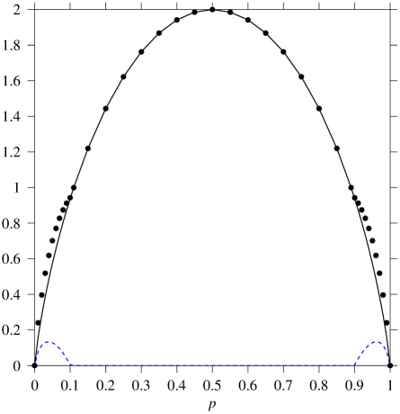
Figure 2: Plots of $K_{E}(U_{p})$ (dots) and $K_{\mathrm{Sch}}(U_{p})$ (solid) as functions of $p$, and of the difference $K_{E}(U_{p})-K_{\mathrm{Sch}}(U_{p})$ (dashed), demonstrating that $K_{E}(U_{p})\neq K_{\mathrm{Sch}}(U_{p})$ for some values of $p$.

We now have the tools required to prove that $K_{E}$ is superadditive, as promised at the end of the last section.

Theorem 8

$K_{E}$ is superadditive, i.e. there exist unitaries $U$ such that

$$K_{E}^{{\cal A}_{1}{\cal A}_{2}:{\cal B}_{1}{\cal B}_{2}}(U_{{\cal A}_{1}{\cal B}_{1}}\otimes U_{{\cal A}_{2}{\cal B}_{2}})>2K_{E}^{{\cal A}_{1}{\cal B}_{1}}(U_{{\cal A}_{1}{\cal B}_{1}}).$$ (57)

where the subscripts on $U$ indicate the subsystems to which it is applied.

Proof: Let $U=\sqrt{1-p}\,I\otimes I+i\sqrt{p}\,X\otimes X$. We show that additivity is violated for certain values of $p$. (We will only add subscripts where necessary.)

Since $U$ has two Schmidt coefficients, Th. 7 implies that $K_{E}(U)=K_{\mathrm{Sch}}(U)$. Therefore, the right-hand side of Eq. (57) is $2K_{E}(U)=2K_{\mathrm{Sch}}(U)=2H(p)$.

To obtain the violation of additivity Eq. (57) we now construct specific states $|\alpha\rangle$ and $|\beta\rangle$ of ${\cal A}$ and ${\cal B}$ for which $E(U|\alpha\rangle|\beta\rangle)>2H(p)$. To do this, we apply $U\otimes U$ to two pairs of systems, as depicted in Fig. 3, where we have omitted the ancillas as they turn out not to be necessary for our construction of $|\alpha\rangle$ and $|\beta\rangle$. Let $|\alpha\rangle=(|00\rangle+|11\rangle)/\sqrt{2}$ be a state of Alice’s system ${\cal A}_{1}{\cal A}_{2}$ and $|\beta\rangle=(|00\rangle+|11\rangle)/\sqrt{2}$ be a state of Bob’s system ${\cal B}_{1}{\cal B}_{2}$.

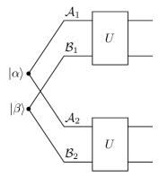
Figure 3: Diagram of $U\otimes U$ applied to systems ${\cal A}_{1}{\cal B}_{1}$ and ${\cal A}_{2}{\cal B}_{2}$. Note that ${\cal A}_{1}{\cal A}_{2}$ starts out in the maximally entangled state $|\alpha\rangle$, and ${\cal B}_{1}{\cal B}_{2}$ starts out in the maximally entangled state $|\beta\rangle$, so ${\cal A}_{1}A_{2}$ is not initially entangled with ${\cal B}_{1}{\cal B}_{2}$.

We make use of a handy identity to calculate $E(U|\alpha\rangle|\beta\rangle)$. Since $|\alpha\rangle$ and $|\beta\rangle$ are maximally entangled, a calculation shows that for any two-qubit unitary $U$,

$$\left(U_{{\cal A}_{1}{\cal B}_{1}}\otimes I_{{\cal A}_{2}{\cal B}_{2}}\right)|\alpha\rangle|\beta\rangle=\left(I_{{\cal A}_{1}{\cal B}_{1}}\otimes U_{{\cal A}_{2}{\cal B}_{2}}^{T}\right)|\alpha\rangle|\beta\rangle,$$ (58)

where the transpose is taken in the basis $\{|00\rangle,|01\rangle,|10\rangle,|11\rangle\}$. This is illustrated in Fig. 4.

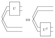
Figure 4: Illustration of the identity $U_{{\cal A}_{1}{\cal B}_{1}}\otimes I_{{\cal A}_{2}{\cal B}_{2}}|\alpha\rangle|\beta\rangle=I_{{\cal A}_{1}{\cal B}_{1}}\otimes U_{{\cal A}_{2}{\cal B}_{2}}^{T}|\alpha\rangle|\beta\rangle$.

For the unitary we are considering, $U^{T}=U$, so that Eq. (58) implies

$$E(U_{{\cal A}_{1}{\cal B}_{1}}\otimes U_{{\cal A}_{2}{\cal B}_{2}}|\alpha\rangle|\beta\rangle)=E(I_{{\cal A}_{1}{\cal B}_{1}}\otimes U_{{\cal A}_{2}{\cal B}_{2}}^{2}|\alpha\rangle|\beta\rangle).$$ (59)

We may now apply Lemma 5, considering ${\cal A}_{1}$ and ${\cal B}_{1}$ as the ancillas to ${\cal A}_{2}$ and ${\cal B}_{2}$, respectively. We see that $E(U_{{\cal A}_{1}{\cal B}_{1}}\otimes U_{{\cal A}_{2}{\cal B}_{2}}|\alpha\rangle|\beta\rangle)=K_{\mathrm{Sch}}(U^{2})$. Observing that $U^{2}$ is a unitary with two Schmidt coefficients,

$$U^{2}=(1-2p)I\otimes I+2i\sqrt{p(1-p)}\,X\otimes X,$$ (60)

we obtain

$$K_{E}(U\otimes U)\geq E(U\otimes U|\alpha\rangle|\beta\rangle)=H\left[(1-2p)^{2}\right],$$ (61)

so we have reduced the problem to showing that there exist values of $p$ such that $H\left[(1-2p)^{2}\right]>2H(p)$. The existence of such values is shown in Fig. 5 . $\blacksquare$

Figure 5: A plot of $2H(p)$, $H\left[(1-2p)^{2}\right]$, and their difference.

V.1.3 Extension to general quantum operations

Our results to this point have primarily concerned strength measures for unitary operations. In this subsection, we obtain some results for general quantum operations, proving generalizations of Lemma 5 and Th. 6 to quantum operations. We will not do a detailed investigation of the axioms and properties satisfied by these measures for general operations, although arguments similar to the unitary case mostly go through.

The first step is to generalize our definitions of $K_{E}$ and $K_{\mathrm{Sch}}$. In order to generalize $K_{E}$ (Eq. (16)) to quantum operations, we must choose an entanglement measure which applies to mixed states as well as pure states. We use the entanglement of formation Wootters (1998):

$$F(\rho)\equiv\min\sum\nolimits_{j}p_{j}E(|\psi_{j}\rangle)$$ (62)

where the minimization is over all pure state decompositions $\{p_{j},|\psi_{j}\rangle\}$ of $\rho$, and $E$ is the entanglement of pure states. Note that any two decompositions of $\rho$ are related by a right unitary matrix $U_{jk}$: $\rho=\sum_{j}p_{j}|\psi_{j}\rangle\langle\psi_{j}|=\sum_{k}q_{k}|\phi_{k}\rangle\langle\phi_{k}|$ if and only if Schrödinger (1936); Jaynes (1957); Hughston et al. (1993) $\sqrt{p_{j}}|\psi_{j}\rangle=\sum_{j}U_{jk}\sqrt{q_{k}}|\phi_{k}\rangle$. We take as our generalized $K_{E}({\cal E})$ the maximum entanglement generated by ${\cal E}$ over all separable input states $\rho_{{\cal A}:{\cal B}}$:

$$K_{E}({\cal E})=\max_{\rho_{{\cal A}:{\cal B}}}F\left[{\cal E}(\rho_{{\cal A}:{\cal B}})\right].$$ (63)

Note that $F\circ{\cal E}$ is a convex function maximized on the convex set of separable states, $\{\rho_{{\cal A}:{\cal B}}\}$, and therefore $F\left[{\cal E}(\rho_{{\cal A}:{\cal B}})\right]$ achieves its maximum for extreme points of the set of separable states, i.e. pure product states.

To generalize $K_{\mathrm{Sch}}$, let ${\cal E}$ be a quantum operation with operation elements $\{G_{k}\}$: ${\cal E}(\rho)=\sum\nolimits_{k}G_{k}\rho G_{k}^{\dagger}$. ${\cal E}$ can be decomposed differently as ${\cal E}(\cdot)=\sum_{j}F_{j}\cdot F_{j}^{\dagger}$ if and only if Choi (1975) the two sets of operation elements are related by a right unitary matrix: $F_{j}=\sum_{k}U_{jk}G_{k}$. By analogy with the entanglement of formation, a natural definition of $K_{\mathrm{Sch}}({\cal E})$ is

$$K_{\mathrm{Sch}}({\cal E})\equiv\min\sum_{j}\frac{\mathrm{tr}(F_{j}^{\dagger}F_{j})}{d_{\cal A}d_{\cal B}}K_{\mathrm{Sch}}(F_{j}),$$ (64)

where $K_{\mathrm{Sch}}(F_{j})$ is given by Eq. (15), and the minimization is over all possible decompositions of ${\cal E}$ into operation elements. The coefficients $\mathrm{tr}(F_{j}^{\dagger}F_{j})/(d_{\cal A}d_{\cal B})$ form a probability distribution. A physical interpretation is as follows: if $K_{\mathrm{Sch}}(F_{j})$ is the strength of the operation $F_{j}$, then $K_{\mathrm{Sch}}({\cal E})$ is the expected strength of ${\cal E}$, minimized over all possible decompositions of ${\cal E}$.

First, we prove two lemmas generalizing Lemma 5. For the remainder of this section, let $|\alpha\rangle$ be a maximally entangled state of system ${\cal A}$ with an ancilla ${\cal R}_{\cal A}$, and $|\beta\rangle$ be a maximally entangled state of ${\cal B}$ with an ancilla ${\cal R}_{\cal B}$.

Lemma 9

For all operators $Q$,

$$K_{\mathrm{Sch}}(Q)=E\left(\textstyle{\sqrt{\frac{d_{\cal A}d_{\cal B}}{\mathrm{tr}(Q^{\dagger}Q)}}}Q|\alpha\rangle|\beta\rangle\right).$$ (65)

Proof: Recall that $K_{\mathrm{Sch}}(Q)=H\left(\left\{s_{l}^{2}/\mathrm{tr}(Q^{\dagger}Q)\right\}\right)$, so we need only calculate the right-hand side of Eq. (65). Expand the state $Q|\alpha\rangle|\beta\rangle$ as

$$Q|\alpha\rangle|\beta\rangle=\sum_{l}s_{l}A_{l}|\alpha\rangle B_{l}|\beta\rangle=\sum_{l}\frac{s_{l}}{\sqrt{d_{\cal A}d_{\cal B}}}|a_{l}\rangle|b_{l}\rangle,$$ (66)

where $\sum_{l}s_{l}A_{l}\otimes B_{l}$ is the Schmidt decomposition for $Q$, and $|a_{l}\rangle\equiv\sqrt{d_{\cal A}}\,A_{l}|\alpha\rangle,|b_{l}\rangle\equiv\sqrt{d_{\cal B}}\,B_{l}|\beta\rangle$ are orthonormal bases for their respective systems. The result follows. $\blacksquare$

Lemma 10

For any quantum operation ${\cal E}$, let $\sigma\equiv{\cal E}(|\alpha\rangle\langle\alpha|\otimes|\beta\rangle\langle\beta|)$. Then $K_{\mathrm{Sch}}({\cal E})=F(\sigma)$, where $F$ is the entanglement of formation.

Proof: Let $F_{j}$ be the set of operation elements for ${\cal E}$ achieving the minimum in the definition of $K_{\mathrm{Sch}}$. Then, applying the definition and Lemma 9, we have

$$\begin{split}K_{\mathrm{Sch}}({\cal E})&=\sum_{j}\frac{\mathrm{tr}(F_{j}^{\dagger}F_{j})}{d_{\cal A}d_{\cal B}}K_{\mathrm{Sch}}(F_{j})\\ &=\sum_{j}\frac{\mathrm{tr}(F_{j}^{\dagger}F_{j})}{d_{\cal A}d_{\cal B}}E\left(\textstyle{\sqrt{\frac{d_{\cal A}d_{\cal B}}{\mathrm{tr}(F_{j}^{\dagger}F_{j})}}}F_{j}|\alpha\rangle|\beta\rangle\right).\end{split}$$ (67)

Noting that

$$\left\{\frac{\mathrm{tr}(F_{j}^{\dagger}F_{j})}{d_{\cal A}d_{\cal B}},\sqrt{\frac{d_{\cal A}d_{\cal B}}{\mathrm{tr}(F_{j}^{\dagger}F_{j})}}F_{j}|\alpha\rangle|\beta\rangle\right\}$$ (68)

is an ensemble for $\sigma$, we deduce that $K_{\mathrm{Sch}}({\cal E})\geq F(\sigma)$. To prove the reverse inequality, suppose $\sigma=\sum_{k}p_{k}|\phi_{k}\rangle\langle\phi_{k}|$ is the minimizing decomposition for the entanglement of formation of $\sigma$. Note that $\sigma$ can also be decomposed as

$$\sigma=\sum\nolimits_{j}F_{j}\left(|\alpha\rangle\langle\alpha|\otimes|\beta\rangle\langle\beta|\right)F_{j}^{\dagger}.$$ (69)

The minimizing decomposition is related to the decomposition from Eq. (69) by a right unitary matrix $U$: $\sqrt{p_{k}}|\phi_{k}\rangle=\sum\nolimits_{j}U_{kj}F_{j}|\alpha\rangle|\beta\rangle$. This unitary freedom is identical to the freedom in the operator-sum decomposition, so the set of elements $G_{k}=\sum_{j}U_{kj}F_{j}$ is also an operator-sum decomposition for ${\cal E}$, as well as giving the minimizing decomposition of $\sigma$, that is $\sqrt{p_{k}}|\phi_{k}\rangle=G_{k}|\alpha\rangle|\beta\rangle$. This gives us the desired inequality,

$$\begin{split}F(\sigma)&=\sum_{k}\frac{\mathrm{tr}(G_{k}^{\dagger}G_{k})}{d_{\cal A}d_{\cal B}}E\left(\textstyle{\sqrt{\frac{d_{\cal A}d_{\cal B}}{\mathrm{tr}(G_{k}^{\dagger}G_{k})}}}G_{k}|\alpha\rangle|\beta\rangle\right)\\ &=\sum_{k}\frac{\mathrm{tr}(G_{k}^{\dagger}G_{k})}{d_{\cal A}d_{\cal B}}K_{\mathrm{Sch}}(G_{k})\\ &\geq K_{\mathrm{Sch}}({\cal E}).\end{split}$$ (70)

$\blacksquare$

The desired bound on $K_{E}$ now follows:

Theorem 11

$K_{E}({\cal E})\geq K_{\mathrm{Sch}}({\cal E})$ for all quantum operations ${\cal E}$.

Proof: The result follows immediately from the previous lemma and the fact that

$$K_{E}({\cal E})=\max F[{\cal E}(\rho_{{\cal A}:{\cal B}})]\geq F\left[{\cal E}(|\alpha\rangle\langle\alpha|\otimes|\beta\rangle\langle\beta|)\right].$$ (71)

$\blacksquare$

V.2 Entanglement generation with prior entanglement

In this section we consider the largest change in entanglement which can be caused by a unitary $U$, using both ancillas and prior entanglement, as defined in Eq. (17) and repeated here for convenience: $K_{\Delta E}(U)=\sup_{|\psi\rangle}|E(U|\psi\rangle)-E(|\psi\rangle)|$, where $U$ acts on the combined system ${\cal A}$${\cal B}$, and $|\psi\rangle$ is an arbitrary state of ${\cal A}$${\cal B}$ plus their ancillas, ${\cal R}_{\cal A}$ and ${\cal R}_{\cal B}$. We show that, although $K_{\Delta E}$ involves a more difficult maximization than $K_{E}$, and may therefore be more difficult to work with, it satisfies more of the axioms and properties described in Sec. III.2 than $K_{E}$ does. Incidentally, since $K_{\Delta E}$ and $K_{E}$ have different properties they can not, in general, be equal.

We first show that $K_{\Delta E}$ obeys the three axioms. $K_{\Delta E}$ is clearly non-negative and satisfies local unitary invariance. To show that $K_{\Delta E}$ satisfies locality is only slightly more involved. If $U=A\otimes B$, then $K_{\Delta E}(A\otimes B)=\sup_{|\psi\rangle}|E(A\otimes B|\psi\rangle)-E(|\psi\rangle)|=0$. On the other hand, since $K_{\Delta E}(U)\geq K_{E}(U)$ and we know that $K_{E}(U)$ satisfies locality, $K_{\Delta E}(U)=0$ only if $K_{E}(U)$, which implies that $U$ is a local unitary, as required.

Second, we show that $K_{\Delta E}$ satisfies Properties 1, 2, 4, and 6–8. Properties 1 and 2, exchange symmetry and time-reversal invariance, are easily seen to be true. We do not know whether property 3, continuity, is satisfied. The argument used to establish that $K_{E}$ is continuous does not work in this instance, because we do not have any bound on the size of the ancilla that ${\cal A}$ and ${\cal B}$ may use. If such a bound could be established then a similar continuity bound to that used for $K_{E}$ could be proved. Next, we show that $K_{\Delta E}$ obeys chaining, Property 4. For any two unitaries $U$ and $V$,

$$\!\!\!\!K_{\Delta E} \!\!\!\!(UV)=\sup_{|\psi\rangle}|E(UV|\psi\rangle)-E(|\psi\rangle)|$$ (72)

$$\!\!\!\!= \!\!\!\!\!\!\sup_{|\psi\rangle}\left|E(UV|\psi\rangle)-E(V|\psi\rangle)+E(V|\psi\rangle)-E(|\psi\rangle)\right|$$

$$\!\!\!\!\leq \!\!\!\!\!\!\sup_{|\phi\rangle=V|\psi\rangle}|E(U|\phi\rangle)-E(|\phi\rangle)|+\sup_{|\psi\rangle}|E(V|\psi\rangle)-E(|\psi\rangle)|$$

$$\!\!\!\!= \!\!\!\!\!\!K_{\Delta E}(U)+K_{\Delta E}(V).$$

Property 6, stability with respect to ancillas, holds since $K_{\Delta E}$ already allows the possibility of arbitrary ancillas. Therefore, by Proposition 2, $K_{\Delta E}$ also satisfies strong subadditivity, Property 8. Finally, we note that the definitions immediately imply that $K_{\Delta E}$ satisfies the reduction property, Property 9.

VI Strength measures based on metrics

In this section we consider a class of strength measures motivated by the axiomatic approach. This is in contrast to Sec. V, where we studied strength measures based on entanglement generation. The strength measures we study here are based on metrics. We explore the axioms and properties obeyed by these measures when different constraints are placed on the underlying metrics. We derive an exact, analytic formula for one particular measure. Finally, we examine the potential of these measures for analyzing quantum computational complexity, as described in Sec. III.2.

Recall the definition of a metric. Let $\mathbb{X}$ be a set. A metric is a real function $D:\mathbb{X}\times\mathbb{X}\to\mathbb{R}$ satisfying the following properties for any three elements $x,y,z$ of $\mathbb{X}$:

$$\begin{split}&(1)\ D(x,y)\geq 0\text{ with equality if and only if }x=y\\ &(2)\ D(x,y)=D(y,x)\ \textbf{(symmetry)}\\ &(3)\ D(x,z)\leq D(x,y)+D(y,z)\ \textbf{(triangle inequality)}\end{split}$$

Given a metric $D$, the corresponding strength measure $K_{D}(U)$ is the minimum distance between $U$ and the set of local unitaries $\mathbb{LU}$:

$$K_{D}(U)=\min_{L\in\mathbb{LU}}D(U,L).$$ (73)

The set $\mathbb{LU}$ varies depending on context. The most common case is where $U$ is a two-qudit unitary acting on the space ${\cal A}$${\cal B}$ and $\mathbb{LU}$ is the set of products of one-qudit unitaries, $K_{D}(U)=\min_{A,B}D(U,A\otimes B)$. Analogues of the definition of $K_{D}$ were introduced to quantify state entanglement by Vedral et al. Vedral et al. (1997), and have been studied in considerable detail, proving to be a fruitful approach to quantifying state entanglement.

More generally, if $U$ acts on a composite of systems, ${\cal A}_{1},{\cal A}_{2},\dots,{\cal A}_{m}$, there are several notions of “local”, which we differentiate with superscripts. For example, suppose $U$ acts on ${\cal A}$${\cal B}$${\cal C}$. One notion of “local unitary” corresponds to unitaries of the form $A\otimes B\otimes C$, so that $K_{D}^{{\cal A}:{\cal B}:{\cal C}}(U)=\min_{A,B,C}D(U,A\otimes B\otimes C)$. A different division into subsystems leads to a different measure: $K_{D}^{{\cal A}:{\cal B}{\cal C}}(U)=\min_{A,B}D(U,A\otimes B)$, where $A$ acts on system ${\cal A}$ but now $B$ is any unitary on ${\cal B}$${\cal C}$.

VI.1 Properties of strength measures based on metrics

One reason for studying strength measures based on metrics is that the properties of the strength measure may be controlled by varying the properties of the underlying metric. We consider strength measures based on: (1) arbitrary metrics; (2) metrics invariant under local unitaries; and (3) metrics invariant under any unitary. Each extra requirement causes the strength measure to obey extra axioms and properties from Sec. III.2. Since we know of no general way to characterize families of metrics, in this section we do not consider any of the properties applying to families (Properties 5–9). Therefore, throughout this section we assume $K_{D}=K_{D}^{{\cal A}:{\cal B}}$.

The metric properties are easily seen to guarantee that the axioms of non-negativity and locality hold for all $K_{D}$. An elegant fact is that the metric properties alone also imply that $K_{D}$ satisfies the continuity property:

Lemma 12

For any two unitaries $U$ and $V$, and any metric $D$, $|K_{D}(U)-K_{D}(V)|\leq D(U,V)$.

Proof: Choose $A$ and $B$ such that $K_{D}(V)=D(V,A\otimes B)$. By definition $K_{D}(U)\leq D(U,A\otimes B)$, and by the triangle inequality $D(U,A\otimes B)\leq D(U,V)+D(V,A\otimes B)=D(U,V)+K_{D}(V)$. Thus $K_{D}(U)\leq D(U,V)+K_{D}(V)$, which may be rearranged to give $K_{D}(U)-K_{D}(V)\leq D(U,V)$. By symmetry, $K_{D}(V)-K_{D}(U)\leq D(U,V)$. $\blacksquare$

If $D$ is locally unitarily invariant, i.e. , $D(U,V)=D[(A\otimes B)U,(A\otimes B)V]=D[U(A\otimes B),V(A\otimes B)]$, then $K_{D}$satisfies local unitary invariance.

Finally, suppose the metric satisfies full unitary invariance, so that $D(U,V)=D(WU,WV)=D(UW,VW)$ for any unitary $W$. Then $K_{D}$ satisfies two additional properties. The first is exchange symmetry, which is easily proved. The second is chaining, $K_{D}(UV)\leq K_{D}(U)+K_{D}(V)$. To see this, suppose $A\otimes B$ and $C\otimes D$ minimize $K_{D}(U)$ and $K_{D}(V)$, respectively. Then

$$K_{D} \!\!\!\!(UV)\leq D\left[UV,(A\otimes B)(C\otimes D)\right]$$ (74)

$$\leq \!\!\!\!D\left[UV,U(C\otimes D)\right]+D\left[U(C\otimes D),(A\otimes B)(C\otimes D)\right]$$

$$= \!\!\!\!D(V,C\otimes D)+D(U,A\otimes B)$$

$$= \!\!\!\!K_{D}(U)+K_{D}(V).$$

VI.2 An explicit formula for the Hilbert-Schmidt strength of a two-qubit unitary

In this section we consider an example of a metric-based strength measure, the Hilbert-Schmidt strength $K_{\mathrm{HS}}$ induced by the unitarily invariant Hilbert-Schmidt norm on operators, $\|Q\|_{{\rm HS}}\equiv\sqrt{\mathrm{tr}(Q^{\dagger}Q)}$. More explicitly, for a bipartite unitary operation $U$ we define

$$K_{\mathrm{HS}}(U)\equiv\min_{A,B}\|U-A\otimes B\|_{{\rm HS}},$$ (75)

where $A$ and $B$ are local unitary operators on the respective subsystems. We now exhibit an explicit formula for the Hilbert-Schmidt strength in the two-qubit case.

The statement of the result is simplified by first making some definitions and observations. Let $U$ be a two-qubit unitary operation with canonical decomposition

$$U=(A_{1}\otimes B_{1})e^{i(\theta_{1}X\otimes X+\theta_{2}Y\otimes Y+\theta_{3}Z\otimes Z)}(A_{2}\otimes B_{2}).$$ (76)

Because of local unitary invariance the Hilbert-Schmidt strength depends only on the parameters $\theta_{j}$, that is, we can ignore the local unitary operations $A_{1,2}$ and $B_{1,2}$. Without loss of generality, we assume $U$ is in canonical form, that is, $A_{1}=B_{1}=A_{2}=B_{2}=I$.

We define $|\phi_{0}\rangle=(|00\rangle+|11\rangle)/\sqrt{2}$, and $|\phi_{j}\rangle\equiv(I\otimes\sigma_{j})|\phi_{0}\rangle$ for $j=1,2,3$ where we write $\sigma_{0},\sigma_{1},\sigma_{2},\sigma_{3}$ to denote $I,X,Y,Z$. Note that the set $|\phi_{j}\rangle$ for $j=0,1,2,3$ is the Bell basis, up to phases. A simple but tedious calculation verifies the useful formula $\langle\phi_{j}|\sigma_{k}\otimes\sigma_{l}|\phi_{j}\rangle=\delta_{kl}H_{jk}$, where the $4\times 4$ matrix $H$ is

$$H=\left[\begin{smallmatrix}1&\ \ 1&-1&\ \ 1\\ 1&\ \ 1&\ \;1&-1\\ 1&-1&-1&-1\\ 1&-1&\ \;1&\ \ 1\end{smallmatrix}\right].$$

The $H$ matrix can also be used to evaluate the eigenvalues of $U$. Because $X\otimes X$, $Y\otimes Y$, and $Z\otimes Z$ are diagonal in the $|\phi_{j}\rangle$ basis, $U$ may be written in diagonal form as $U=\sum_{j}\lambda_{j}|\phi_{j}\rangle\langle\phi_{j}|$, where $\lambda_{j}$ are the eigenvalues of $U$. These eigenvalues are evaluated as follows:

$$\begin{split}\lambda_{j}&=\langle\phi_{j}|U|\phi_{j}\rangle\\ &=\left\langle\phi_{j}\left|e^{i(\theta_{1}X\otimes X+\theta_{2}Y\otimes Y+\theta_{3}Z\otimes Z)}\right|\phi_{j}\right\rangle\\ &=\exp\left(i\sum_{k=1}^{3}\theta_{k}\langle\phi_{j}|\sigma_{k}\otimes\sigma_{k}|\phi_{j}\rangle\right),\end{split}$$ (77)

where in the last line we used the fact that all three $\sigma_{k}\otimes\sigma_{k}$ are diagonal in the $|\phi_{j}\rangle$ basis. Substituting $\langle\phi_{j}|\sigma_{k}\otimes\sigma_{l}|\phi_{j}\rangle=\delta_{kl}H_{jk}$ we obtain:

$$\lambda_{j}=\exp\left(i\sum_{k=1}^{3}H_{jk}\theta_{k}\right).$$ (78)

Theorem 13

For a two-qubit unitary $U$ with canonical decomposition Eq. (76), the Hilbert-Schmidt strength is given by the formula

$$K_{\mathrm{HS}}(U)=\sqrt{8-2\max_{0\leq k\leq 3}\textstyle{\left|\sum_{j}\lambda_{j}H_{jk}\right|}}.$$ (79)

The minimizing local unitary is $A\otimes B=e^{i\theta}\sigma_{k}\otimes\sigma_{k}$ where $k$ achieves the maximum in the expression above, and $\theta$ is the argument of $\sum\nolimits_{j}\lambda_{j}H_{jk}$.

Proof: Simple algebra shows that

$$K_{\mathrm{HS}}(U)^{2}=\min_{A,B}\left[8-2\Re\left(\mathrm{tr}\left[U^{\dagger}(A\otimes B)\right]\right)\right],$$ (80)

where $\Re(\cdot)$ denotes the real part. We expand $A$ and $B$ in terms of the Pauli operators as $A=\sum_{k=0}^{3}a_{k}\sigma_{k}$, $B=\sum_{l=0}^{3}b_{l}\sigma_{l}$. (Note that the unitarity of $A$ and $B$ implies that $\sum_{k}|a_{k}|^{2}=\sum_{l}|b_{l}|^{2}=1$.) Substituting these expressions for $A$ and $B$, and $U=\sum_{j}\lambda_{j}|\phi_{j}\rangle\langle\phi_{j}|$, gives

$$K_{\mathrm{HS}}(U)^{2}=\min_{a_{k},b_{l}}\left[8-2\Re\left(\sum_{jkl}\lambda_{j}^{*}a_{k}b_{l}\langle\phi_{j}|\sigma_{k}\otimes\sigma_{l}|\phi_{j}\rangle\right)\right],$$ (81)

where the minimization is over all $a_{k},b_{l}$ such that the corresponding $A$ and $B$ are unitary. But $\langle\phi_{j}|\sigma_{k}\otimes\sigma_{l}|\phi_{j}\rangle\rangle=\delta_{kl}H_{jk}$, as noted earlier, so this expression simplifies to

$$K_{\mathrm{HS}}(U)^{2}=8-2\max_{a_{k},b_{k}}\Re\left(\textstyle{\sum_{jk}\lambda_{j}^{*}a_{k}b_{k}H_{jk}}\right).$$ (82)

The Cauchy-Schwarz inequality implies $\sum_{k}|a_{k}b_{k}|\leq 1$, so:

$$\Re\left(\textstyle{\sum_{jk}\lambda_{j}^{*}a_{k}b_{k}H_{jk}}\right)\!\!\!\!\!\! \leq\sum\nolimits_{k}\left(|a_{k}b_{k}|\left|\sum\nolimits_{j}\lambda_{j}^{*}H_{jk}\right|\right)$$ (83)

$$\leq\max_{k}\left|\sum\nolimits_{j}\lambda_{j}^{*}H_{jk}\right|$$

$$=\max_{k}\left|\sum\nolimits_{j}\lambda_{j}H_{jk}\right|.$$

Equality occurs when $a_{l}=\delta_{kl}$ and $b_{l}=\delta_{kl}e^{i\theta}$, where $k$ maximizes the right-hand side of the inequality, and $e^{i\theta}\sum\nolimits_{j}\lambda_{j}^{*}H_{jk}=\left|\sum\nolimits_{j}\lambda_{j}H_{jk}\right|$. This corresponds to $A\otimes B=e^{i\theta}\sigma_{k}\otimes\sigma_{k}$, and $\theta$ as described in the statement of the theorem. $\blacksquare$

VI.3 Applications to computational complexity

We have seen that strength measures based on unitarily invariant metrics satisfy many desirable axioms and properties. It is natural to ask whether these measures might be useful in answering questions about computational complexity, as described in Sec. III.2.

In order for a family of measures {$K_{D}$} to be useful in this context, we require {$K_{D}$} to be stable under addition of systems (for the remainder of this section, we simply write “stable” for this property). This is to ensure that the strength of a cnot gate is independent of the number of qubits in the system being studied. It is tempting to consider a family of measures {$K_{D}$} whose underlying family of metrics is stable, in the sense that $D(U,V)=D(U\otimes I,V\otimes I)$ for any unitaries $U$ and $V$. However, we show here that such metrics give rise to trivial bounds on computational complexity. Denote by $U$ a unitary acting on $n$ qubits, and let $0$ and $I$ be the zero and identity operator, respectively, on $n$ qubits. For any such unitary,

$$K_{D}(U) = \min_{A_{1},\ldots,A_{n}}D(U,A_{1}\otimes\ldots\otimes A_{n})$$ (84)

$$\leq \min_{A_{1},\ldots,A_{n}}\left[D(U,0)+D(0,A_{1}\otimes\ldots\otimes A_{n})\right]$$

$$= 2D(I,0),$$

where to obtain the last line we used the unitary invariance of $D$. But $I=I_{1}\otimes I_{2}\otimes\cdots\otimes I_{n}$, where $I_{j}$ is the identity on the $j$th qubit, so by the metric stability property $K_{D}(U)$ is always bounded by $2D(I,0)=2D(I_{1},0)$, which is a constant. Therefore, the lower bound on the number of two-qubit gates required to implement a $n$-qubit gate, $k\geq K(U)/K_{\max}$ (Eq. (22)), is a constant.

This shows that any family of metrics which is both unitarily invariant and stable cannot give interesting lower bounds on computational complexity. As noted above, unitary invariance is a useful property. On the other hand, stability of the family of metrics may not be necessary for stability of the induced family of measures. So, it may be possible to find a family of unitarily invariant metrics which is not stable, but which induces a stable family of measures, and could therefore give useful lower bounds on computational complexity.

Measure:	$K_{\mathrm{Har}}$	$K_{\mathrm{Sch}}$	$K_{E}$	$K_{\Delta E}$	$K_{D}$	$K_{D}$[LU]	$K_{D}$[U]
A1 Non-negativity	yes	yes	yes	yes	yes	yes	yes
A2 Locality	yes	yes	yes	yes	yes	yes	yes
A3 LU invariance	yes	yes	yes	yes	?	yes	yes
P1 Exchange	yes	yes	yes	yes	?	?	yes
P2 Time-reversal	yes	yes	?	yes	?	?	?
P3 Continuity	no	yes	yes	?	yes	yes	yes
P4 Chaining	yes	no	no	yes	?	?	yes
P5 System stability	–	–	–	–	?	?	?
P6 Ancilla stability	yes	yes	yes	yes	?	?	?
P7 Weak additivity	yes	yes	no	yes	?	?	?
P8 Strong additivity	yes	yes	no	yes	?	?	?
P9 Reduction	yes	no	yes	yes	?	?	?

Table 1: Summary of axioms and properties of strength measures. “yes”/”no” indicates whether the strength measure obeys the axiom/property. “–” means the property is not applicable, and “?” means we do not know whether the strength measure obeys the axiom/property. $K_{D}$[LU] refers to strength measures induced by locally unitarily invariant metrics, and $K_{D}$[U] refers to strength measures induced by unitarily invariant metrics.

VII Summary and future directions

We have developed the beginnings of a quantitative theory of quantum dynamical operations as a physical resource. While promising preliminary results have been obtained, an enormous amount of work remains to be done. (Table 1 summarizes the properties of the strength measures we investigated.) We believe the development of this theory offers a concrete path to address the fundamental question of quantum computational complexity: how many one- and two-qubit quantum operations are required to do some desired quantum operation ${\cal E}$? This will, in turn, allow us to answer questions about the relationship of quantum and classical complexity classes, and may enable the resolution of some longstanding questions in complexity theory.

Acknowledgments We thank Charlene Ahn, Sean Barrett, Tony Bracken, Andrew Childs, and Xiaoguang Wang for helpful discussions. MAN thanks Raymond Laflamme for an enjoyable 1998 discussion about the idea of quantifying the “entangling power” of a quantum dynamical operation. AWH acknowledges support from the NSA and ARDA under ARO contract no. DAAD19-01-1-06, and thanks the other authors for their hospitality.

References

- Bennett et al. (1996) C. H. Bennett, D. P. DiVincenzo, J. A. Smolin, and W. K. Wootters, Phys. Rev. A 54, 3824 (1996).
- Schumacher and Westmoreland (2002) B. Schumacher and M. D. Westmoreland, arXiv:quant-ph/0201061 (2002).
- Horodecki et al. (1999) M. Horodecki, P. Horodecki, and R. Horodecki, Phys. Rev. A 60, 1888 (1999).
- Nielsen (1998) M. A. Nielsen, Ph.D. thesis, University of New Mexico (1998), arXiv:quant-ph/0011036.
- Nielsen and Chuang (2000) M. A. Nielsen and I. L. Chuang, Quantum computation and quantum information (Cambridge University Press, Cambridge, 2000).
- Nielsen (2002) M. A. Nielsen, arXiv:quant-ph/0210005 (2002).
- Osborne (2002) T. J. Osborne, Ph.D. thesis, The University of Queensland (2002), submitted in July.
- Dodd et al. (2002) J. L. Dodd, M. A. Nielsen, M. J. Bremner, and R. T. Thew, Phys. Rev. A 65, 040301(R) (2002).
- Wocjan et al. (2002) P. Wocjan, D. Janzing, and T. Beth, Quantum Information and Computation 2, 117 (2002).
- Dür et al. (2001) W. Dür, G. Vidal, J. I. Cirac, N. Linden, and S. Popescu, Phys. Rev. Lett. 87, 137901 (2001).
- Bennett et al. (2001) C. H. Bennett, J. I. Cirac, M. S. Leifer, D. W. Leung, N. Linden, S. Popescu, and G. Vidal, arXiv:quant-ph/0107035 (2001).
- Nielsen et al. (2001) M. A. Nielsen, M. J. Bremner, J. L. Dodd, A. M. Childs, and C. M. Dawson, Phys. Rev. A 66, 022317 (2002).
- Vidal et al. (2002a) G. Vidal, K. Hammerer, and J. I.Cirac, Phys. Rev. Lett. 88, 237902 (2002a).
- Jones and Knill (1999) J. A. Jones and E. Knill, Journal of Magnetic Resonance 141, 322 (1999).
- Leung et al. (2000) D. W. Leung, I. L. Chuang, F. Yamaguchi, and Y. Yamamoto, Phys. Rev. A 61, 042310 (2000).
- Brylinski and Brylinski (2002) J. L. Brylinski and R. Brylinski, Universal quantum gates (2002), chap. II in Brylinski and Chen (2002), arXiv:quant-ph/0108062.
- Bremner et al. (2002) M. J. Bremner, C. M. Dawson, J. L. Dodd, A. Gilchrist, A. Harrow, D. Mortimer, M. A. Nielsen, and T. J. Osborne (2002), arXiv:quant-ph/0207072.
- Eisert et al. (2000) J. Eisert, K. Jacobs, P. Papadopoulos, and M. B. Plenio, Phys. Rev. A 62, 052317 (2000).
- Collins et al. (2001) D. Collins, N. Linden, and S. Popescu, Phys. Rev. A 64, 032302 (2001).
- Chefles et al. (2001) A. Chefles, C. R. Gilson, and S. M. Barnett, Phys. Rev. A 63, 032314 (2001).
- Makhlin (2000) Y. Makhlin, arXiv:quant-ph/0002045 (2000).
- Zanardi et al. (2000) P. Zanardi, C. Zalka, and L. Faoro, Phys. Rev. A 62, 030301(R) (2000).
- Zanardi (2001) P. Zanardi, Phys. Rev. A 63, 040304(R) (2001).
- Wang and Zanardi (2002) X. Wang and P. Zanardi, arXiv:quant-ph/0207007 (2002).
- Cirac et al. (2000) J. I. Cirac, W. Dür, B. Kraus, and M. Lewenstein, Phys. Rev. Lett. 86, 544 (2000).
- Kraus and Cirac (2001) B. Kraus and J. I. Cirac, Phys. Rev. A 63, 062309 (2001).
- Leifer et al. (2002) M. S. Leifer, L. Henderson, and N. Linden, arXiv:quant-ph/0205055 (2002).
- Scarani et al. (2002) V. Scarani, M. Ziman, P. Štelmachovič, N. Gisin, and V. Bužek, Phys. Rev. Lett. 88, 097905 (2002).
- Vidal et al. (2002b) G. Vidal, K. Hammerer, and J. I. Cirac, Phys. Rev. Lett. 88, 237902 (2002b).
- Hammerer et al. (2002) K. Hammerer, G. Vidal, and J. I. Cirac, arXiv:quant-ph/0205100 (2002).
- Childs et al. (2002) A. M. Childs, D. W. Leung, F. Verstraete, and G. Vidal, arXiv:quant-ph/0207052 (2002).
- Beckman et al. (2001) D. Beckman, D. Gottesman, M. A. Nielsen, and J. Preskill, Phys. Rev. A 64, 052309 (2001).
- Bennett et al. (2002) C. H. Bennett, A. Harrow, D. W. Leung, and J. A. Smolin, arXiv:quant-ph/0205057 (2002).
- Berry and Sanders (2002) D. W. Berry and B. C. Sanders, arXiv:quant-ph/0207065 (2002).
- Shor (1994) P. Shor, in Proc. 35th Annual Symposium on Foundations of Computer Science (IEEE Computer Society Press, Los Alamitos, CA, 1994), p. 124.
- Hill and Wootters (1997) S. Hill and W. K. Wootters, Phys. Rev. Lett. 78, 5022 (1997).
- Vedral et al. (1997) V. Vedral, M. B. Plenio, M. A. Rippin, and P. L. Knight, Phys. Rev. Lett. 78, 2275 (1997).
- Vedral and Plenio (1998) V. Vedral and M. B. Plenio, Phys. Rev. A 57, 1619 (1998).
- Vidal (2000) G. Vidal, Journal of Modern Optics 47, 355 (2000).
- Nielsen (2000a) M. A. Nielsen, Journal of Physics A 34, 6987 (2000a).
- Popescu and Rohrlich (1997) S. Popescu and D. Rohrlich, Phys. Rev. A 56, R3319 (1997).
- Nielsen (2000b) M. A. Nielsen, Phys. Rev. A 61, 064301 (2000b).
- Lieb and Ruskai (1973) E. H. Lieb and M. B. Ruskai, J. Math. Phys. 14, 1938 (1973).
- Barenco et al. (1995) A. Barenco, C. H. Bennett, R. Cleve, D. P. DiVincenzo, N. Margolus, P. Shor, T. Sleator, J. A. Smolin, and H. Weinfurter, Phys. Rev. A 52, 3457 (1995).
- Yao (1993) A. C. Yao, Proc. of the 34th Ann. IEEE Symp. on Foundations of Computer Science pp. 352–361 (1993).
- Kremer (1995) I. Kremer, Master’s thesis, The Hebrew University of Jerusalem (1995).
- Mehlhorn and Schmidt (1982) K. Mehlhorn and E. Schmidt, Proc. of 14th ACM Symposium on Theory of Computing pp. 330–337 (1982).
- Kushilevitz and Nisan (1997) E. Kushilevitz and N. Nisan, Communication Complexity (Cambridge University Press, Cambridge, 1997).
- Buhrman et al. (1998) H. Buhrman, R. Cleve, and A. Wigderson, arXiv:quant-ph/9802040 (1998).
- Buhrman and de Wolf (1999) H. Buhrman and R. de Wolf, arXiv:cs.CC/9910010 (1999).
- Bennett (1973) C. H. Bennett, IBM Journal of Research and Development 17, 525 (1973).
- Cleve et al. (1997) R. Cleve, W. van Dam, M. A. Nielsen, and A. Tapp, arXiv:quant-ph/9708019 (1997).
- Khaneja et al. (2001) N. Khaneja, R. Brockett, and S. J. Glaser, Phys. Rev. A 63, 032308 (2001).
- Horn and Johnson (1991) R. A. Horn and C. R. Johnson, Topics in matrix analysis (Cambridge University Press, Cambridge, 1991).
- Donald and Horodecki (1999) M. J. Donald and M. Horodecki, Phys. Lett. A 264, 257 (1999).
- Wootters (1998) W. K. Wootters, Phys. Rev. Lett. 80, 2245 (1998).
- Schrödinger (1936) E. Schrödinger, Proc. Cambridge Phil. Soc. 32, 446 (1936).
- Jaynes (1957) E. T. Jaynes, Phys. Rev. 108, 171 (1957).
- Hughston et al. (1993) L. P. Hughston, R. Jozsa, and W. K. Wootters, Phys. Lett. A 183, 14 (1993).
- Choi (1975) M.-D. Choi, Linear Algebra and Its Applications 10, 285 (1975).
- Brylinski and Chen (2002) R. K. Brylinski and G. Chen, eds., Mathematics of Quantum Computation, Computational Mathematics (Chapman & Hall / CRC Press, 2002).
- Terhal and Horodecki (2000) B. M. Terhal and P. Horodecki, Phys. Rev. A 61, 040301 (2000).
- Press et al. (1992) W. H. Press, S. A. Teukolsky, W. T. Vetterling, and B. P. Flannery, Numerical Recipes in C (Cambridge University Press, Cambridge, 1992), 2nd ed.
- Griffiths and Niu (1996) R. B. Griffiths and C.-S. Niu, Phys. Rev. Lett. 76, 3228 (1996).
- Tyson (2002) J. Tyson, arXiv:quant-ph/0210100 (2002).
- Hartley (1928) R. V. L. Hartley, Bell Systems Technical Journal 7, 535 (1928).
- Dür et al. (2002) W. Dür, G. Vidal, and J. I. Cirac, Phys. Rev. Lett. 89, 057901 (2002).