Cooperative three- and four- player quantum games

Abstract

A cooperative multi-player quantum game played by 3 and 4 players has been studied. Quantum superposed operator is introduced in this work which solves the non-zero sum difficulty in previous treatment. The role of quantum entanglement of the initial state is discussed in details.

I Introduction

Quantum game theory has become a new area of application of quantum theory. It has attracted much attention. Among them, two-player quantum game [1, 2], multi-player non-cooperative quantum game [3] and the cooperative three player quantum game [4] have been reported recently. The prisoner’s dilemma game has been demonstrated recently in NMR experiment[5]. In classical game theory, the cooperation of the players means that they can exchange completely information with one another, and they take the strategy to the most behoof of themselves. In this way, co-operators can be seen as one player. It is very important in cooperative game that each party in a cooperation must take coordinated strategies. For this purpose, in game theory, Nash equilibrium(NE) is an important concept. In an Nash equilibrium, each player obtains his/her optimal payoff, and if he/she tries to change his/her strategy from the NE strategy, his/her payoff will become less. In cooperative quantum game, the situation is similar.

In this paper, we study a game played by 3 and 4 players. The rules for the cooperative 3 player game were given in Ref.[4]. Suppose that there are three players denoted as $N=\{A,B,C\}$, where $A$ and $B$ are cooperators are $C$ is solitary. Each player has a strategy set $S_{i}(i=A,B,C)$. The payoff set for the corresponding strategies is $P_{i}(i=A,B,C)$. It is a function of the strategy $S_{A}\times S_{B}\times S_{C}$. Each player can choose one of the two strategies denoted as $0$ and $1$. In each play, if there is a player uses the minority strategy, then this player is a looser and he/she has to give one penny to each of the other two players. In the 4 player cooperative game, the model and the rules are similar. But in this case, there is a possibility that every two players choose the same strategy, then there is no gain or loss for anyone.

In the quantum version of this game, an multi-qubit initial quantum state is prepared by an arbiter and the qubits are sent to all players at random, one qubit for each player. It is assumed that each player possesses local unitary operators $i.e.$ $I$ and $\sigma_{x}$ on their own qubit at their proposal, and then sends the qubit back to the arbiter. Upon receiving all the qubits, the arbiter will measure them to get the results and distribute the payoff to each player. In this work, we studied two different ways each player performs his/her strategies. In the classical probability operator(CPO) way, each player is allowed to perform $I$ and $\sigma_{x}$ with probability $p$ and $1-p$ respectively. In CPO, the players work exactly the way as in a classical game. The only difference is that they lay their bet on a quantum state. In Ref.[4, 6, 7], the strategy is performed in this way. In a quantum superposed operator(QSO) way, each player is allowed to perform an unitary operation that is a linear combination of $I$ and $\sigma_{x}$: $\sqrt{p}I+\sqrt{1-p}\sigma_{x}$. This corresponds to a physical implementation that each player is allowed to use linear superposition of the identity operator and the $\sigma_{x}$. Acting upon state $|0\rangle$, it produces $\sqrt{p}|0\rangle+\sqrt{1-p}|1\rangle$. If one makes measurement on this state, he/she will have $p$ probability to obtain 0, and $1-p$ probability to obtain 1. This is closely related to CPO and classical game with $p$ probability to choose 0 and $1-p$ probability to choose 1. The cooperative quantum game between 3 players using CPO has been studied in Ref.[4]. In our work, we study the 3 and 4 player quantum minority game using QSO and the 4 player game using CPO. We found that qualitatively, QSO and CPO produce the same outcome, but they differ in details in quantity. It is found that in a cooperative quantum game, the initial state plays a crucial role. For some initial state, cooperation is very important. For some other initial state, cooperation becomes useless. This is quite different from what we know in a classical game theory.

II Three-player cooperative game in QSO

Now we come to the three cooperative quantum game (TCQG). The players implement their strategies by applying the identity operator $I$ and the $Pauli$-spin flip $\sigma_{x}.$ The three player cooperative game with CPO has been studied in Ref. [4]. Here we will discuss this game with QSO. We assume that the cooperators take the correlated operations to the their qubits. Now suppose the initial state is $|\psi_{0}\rangle$=$c_{1}|000\rangle$+$c_{2}|111\rangle$, where $c_{1}^{2}+c_{2}^{2}=1$, $c_{1}\geq 0$, $c_{2}\geq 0$. Because $A$ and $B$ are cooperators, in term of the rules, they take the same strategies, so they do the same operations on their respective qubits: $\sqrt{p}II+\sqrt{1-p}\sigma_{x}\sigma_{x}$. $C\ \$takes operation $\sqrt{q}I+\sqrt{1-q}\sigma_{x}$. After the operations have been performed, the state of the system becomes

$$\psi_{out} = (c_{1}\sqrt{pq}+c_{2}\sqrt{(1-p)(1-q)})|000\rangle$$ (4)

$$+(c_{1}\sqrt{p(1-q)}+c_{2}\sqrt{(1-p)q})|001\rangle$$

$$+(c_{1}\sqrt{(1-p)q}+c_{2}\sqrt{p(1-q)})|110\rangle$$

$$+(c_{1}\sqrt{(1-p)(1-q)}+c_{2}\sqrt{pq})|111\rangle.$$

The payoff of player A is the sum of squares of the coefficients of $|001\rangle$ and $|110\rangle$:

$$P_{A}=p+q-2pq+4c_{1}c_{2}\sqrt{p(1-p)q(1-q)}=p+q-2pq+4a\sqrt{p(1-p)q(1-q)},$$ (5)

where $a=c_{1}c_{2}$. We have plotted the payoff of A with respect to $p$ and $q$ in Fig.1. “$a$” is a measure of entanglement of the initial state. When “$a$”=0, the initial state is a product state and there is no entanglement in it. We see from Fig.1a that there is clearly a saddle point in the 3-dimensional figure. As “$a$” increases to $1/3$, the saddle point becomes shallower(Fig.1b). When “$a$”=1, the system has maximum entanglement, and the saddle becomes flat(Fig.1c). This clearly shows that the initial state is very important in the cooperative game. The 3D-figure displays a shape of saddle, and the saddle-point is just the NE point. To gain the optimal payoff, we let

$$\frac{\partial P_{A}}{\partial p} = 1-2q+2a\sqrt{\frac{q(1-q)}{p(1-p)}}(1-2p)=0,$$ (6)

$$\frac{\partial P_{A}}{\partial q} = 1-2p+2a\sqrt{\frac{p(1-p)}{q(1-q)}}(1-2q)=0.$$ (7)

Combining Eqs.(6, 7), we can get $p=q=1/2$. Substituting into Eq.(5), then the payoff $A$ can get is

$$P_{A,max}=1/2+a.$$ (8)

The relation between $P_{A,max}$ and $a$ is shown in Fig. 2. Similarly, the payoff of $B$ and $C$ are:

$$P_{B} = P_{A}=1/2+a,$$ (9)

$$P_{C} = -2P_{A}=-1-2a.$$ (10)

For players $A$ and $B$, the larger the numerical value of $a$, the more their payoff. The payoff of player $A$ varies continuously with the change in the value of $a$. When $a=0$, in other words, the initial state is $|000\rangle$ or $|111\rangle$, the payoff is the same as that in a classical game, $viz$ the payoff is 0.5. When the initial state has maximum entanglement, his payoff achieves the maximum, 1. Thus, cooperation must have more advantage for $A$ and $B$, and their cooperation will be all to nothing going on. Certainly, $P_{A}+P_{B}+P_{C}=0$, that is, our scheme is still a zero-sum game but that in Ref. [4] is not.

In fact, when the initial state is $c_{1}|001\rangle$+$c_{2}|110\rangle$, we can use the same method to find out the equilibrium point. Similarly, the players can take the strategies described above. Then,

$$\psi_{out} = \ \quad(c_{1}\sqrt{p(1-q)}+c_{2}\sqrt{(1-p)q})|000\rangle$$ (13)

$$+(c_{1}\sqrt{(1-p)(1-q)}+c_{2}\sqrt{pq})|110\rangle$$

$$+(c_{1}\sqrt{(1-p)q}+c_{2}\sqrt{p(1-q)})|111\rangle.$$

In term of this equation, we can write the payoff of $A$:

$$P_{A}=1-p-q+2pq+4a\sqrt{p(1-p)q(1-q)}.$$ (14)

The relation between $P_{A}$ and these parameters can be seen from Fig. 3. The saddle-point still exists. We can find out the maximum payoff by solving the following equations:

$$\frac{\partial P_{A}}{\partial p} = -1+2q+2a\frac{q(1-q)(1-2p)}{\sqrt{p(1-p)q(1-q)}},$$ (15)

$$\frac{\partial P_{A}}{\partial q} = -1+2p+2a\frac{p(1-p)(1-2q)}{\sqrt{p(1-p)q(1-q)}}.$$ (16)

We get the saddle-point at $p=1/2$ and $q=1/2$, and then $P_{A}=1/2+a$, $P_{B}=1/2+a$, $P_{C}=-1-2a$. The result is the same as that discussed just above. In the classical game, the NE strategy is a point, and so is their corresponding payoff. But in the quantum game, their NE strategies depend on the initial entangle state. Furthermore, in this situation, the cooperation must be of advantage for players $A$ and $B$, and this is the very reason for their continuance of cooperation.

III Four-player cooperative quantum game in CPO

Up to now, no one has studied the four cooperative quantum game (FCQG). In this section we will investigate FCQG in CPO. Here what the players do is similar to that metioned above. The initial state $|\psi_{in}\rangle=\sum_{i,j,k,l=0}^{1}{C}_{ijkl}{|}ijkl{\rangle}$, where $\sum_{i,j,k,l=0}^{1}\left|C_{ijkl}\right|^{2}=1$. Each player takes operation $I$ with classical probabilities $p$,$q$, $r$, $l$, respectively, but the $Pauli$-spin-flip operator $\sigma_{x}$ with probabilities $1-p$, $1-q$, $1-r$, $1-l,$ respectively. After the performance of the strategies, the state of the system changes from $|\psi_{in}\rangle$ to an mixed state represented by a density operator, $\rho=\sum_{i,j,k,l=0}^{1}{|}P_{ijkl}{|^{2}|}ijkl{\rangle\langle}ijkl{|}$. In fact, the state becomes an mixed state when player take strategy in CPO manner. For convenience, the following notations are introduced: $P_{0}=|P_{0000}|^{2}$, $P_{1}=|P_{0001}|^{2}$, $\cdots$, $P_{15}=|P_{1111}|^{2}$, which are the probabilities of the system ending up at state $[0000]$, $[0001]$, $...$, $[1111]$ respectively. $x_{0}=|C_{0000}|^{2}$, $x_{1}=|C_{0001}|^{2}$, $\cdots$, $x_{15}=|C_{1111}|^{2}$ are the probabilities of the system being in state $|0000\rangle$, $|0001\rangle$, $...$, $|1111\rangle$ respectively. The relation between these quantities is

$$Q=\Lambda\;\Pi^{T},$$ (17)

where

$$Q=\left[P_{0},P_{1},\cdots,P_{15}\right]^{T}$$ (18)

and

$$\Pi = [pqrl,pqr\bar{l},pq\bar{r}l,pq\bar{r}\bar{l},p\bar{q}rl,p\bar{q}r\bar{l},p\bar{q}\bar{r}l,p\bar{q}\bar{r}\bar{l},\bar{p}qrl,\bar{p}qr\bar{l},\bar{p}q\bar{r}l,\bar{p}q\bar{r}\bar{l},\bar{p}\bar{q}rl,\bar{p}\bar{q}r\bar{l},\bar{p}\bar{q}\bar{r}l,\bar{p}\bar{q}\bar{r}\bar{l}],$$ (19)

where a bar over a character means 1 minus this quantity, e.g. $\bar{p}=1-p$. The matrix $\Lambda$ is calculated as follows

$$\Lambda=\left[\begin{array}[]{cccccccccccccccc}x_{0}&x_{1}&x_{2}&x_{3}&x_{4}&x_{5}&x_{6}&x_{7}&x_{8}&x_{9}&x_{10}&x_{11}&x_{12}&x_{13}&x_{14}&x_{15}\\ x_{1}&x_{0}&x_{3}&x_{2}&x_{5}&x_{4}&x_{7}&x_{6}&x_{9}&x_{8}&x_{11}&x_{10}&x_{13}&x_{12}&x_{15}&x_{14}\\ x_{2}&x_{3}&x_{0}&x_{1}&x_{6}&x_{7}&x_{4}&x_{5}&x_{10}&x_{11}&x_{8}&x_{9}&x_{14}&x_{15}&x_{12}&x_{13}\\ x_{3}&x_{2}&x_{1}&x_{0}&x_{7}&x_{6}&x_{5}&x_{4}&x_{11}&x_{10}&x_{9}&x_{8}&x_{15}&x_{14}&x_{13}&x_{12}\\ x_{4}&x_{5}&x_{6}&x_{7}&x_{0}&x_{1}&x_{2}&x_{3}&x_{12}&x_{13}&x_{14}&x_{15}&x_{8}&x_{9}&x_{10}&x_{11}\\ x_{5}&x_{4}&x_{7}&x_{6}&x_{1}&x_{0}&x_{3}&x_{2}&x_{13}&x_{12}&x_{15}&x_{14}&x_{9}&x_{8}&x_{11}&x_{10}\\ x_{6}&x_{7}&x_{4}&x_{5}&x_{2}&x_{3}&x_{0}&x_{1}&x_{14}&x_{15}&x_{12}&x_{13}&x_{10}&x_{11}&x_{8}&x_{9}\\ x_{7}&x_{6}&x_{5}&x_{4}&x_{3}&x_{2}&x_{1}&x_{0}&x_{15}&x_{14}&x_{13}&x_{12}&x_{11}&x_{10}&x_{9}&x_{8}\\ x_{8}&x_{9}&x_{10}&x_{11}&x_{12}&x_{13}&x_{14}&x_{15}&x_{0}&x_{1}&x_{2}&x_{3}&x_{4}&x_{5}&x_{6}&x_{7}\\ x_{9}&x_{8}&x_{11}&x_{10}&x_{13}&x_{12}&x_{15}&x_{14}&x_{1}&x_{0}&x_{3}&x_{2}&x_{5}&x_{4}&x_{7}&x_{6}\\ x_{10}&x_{11}&x_{8}&x_{9}&x_{14}&x_{15}&x_{12}&x_{13}&x_{2}&x_{3}&x_{0}&x_{1}&x_{6}&x_{7}&x_{4}&x_{5}\\ x_{11}&x_{10}&x_{9}&x_{8}&x_{15}&x_{14}&x_{13}&x_{12}&x_{3}&x_{2}&x_{1}&x_{0}&x_{7}&x_{6}&x_{5}&x_{4}\\ x_{12}&x_{13}&x_{14}&x_{15}&x_{8}&x_{9}&x_{10}&x_{11}&x_{4}&x_{5}&x_{6}&x_{7}&x_{0}&x_{1}&x_{2}&x_{3}\\ x_{13}&x_{12}&x_{15}&x_{14}&x_{9}&x_{8}&x_{11}&x_{10}&x_{5}&x_{4}&x_{7}&x_{6}&x_{1}&x_{0}&x_{3}&x_{2}\\ x_{14}&x_{15}&x_{12}&x_{13}&x_{10}&x_{11}&x_{8}&x_{9}&x_{6}&x_{7}&x_{4}&x_{5}&x_{2}&x_{3}&x_{0}&x_{1}\\ x_{15}&x_{14}&x_{13}&x_{12}&x_{11}&x_{10}&x_{9}&x_{8}&x_{7}&x_{6}&x_{5}&x_{4}&x_{3}&x_{2}&x_{1}&x_{0}\end{array}\right].$$ (20)

The matrix is symmetric. The payoff of the players $A$, $B$, $C$, $D$ in each basis state $|i\rangle$ are denoted as $\alpha_{i}$, $\beta_{i}$, $\gamma_{i}$, $\theta_{i}$, where range of $i$ is from $0$ through $15$. For instance for player $A$, the payoff in the basis states are

$$\alpha_{0}=\alpha_{3}=\alpha_{5}=\alpha_{6}=\alpha_{9}=\alpha_{10}=\alpha_{12}=\alpha_{5}=0,$$ (21)

$$\alpha_{1}=\alpha_{2}=\alpha_{4}=\alpha_{11}=\alpha_{13}=\alpha_{14}=1,\alpha_{7}=\alpha_{8}=-3.$$ (22)

In the end of the game, the payoff function of player $A$ is

$$P_{A} = \sum_{i=0}^{15}P_{i}\alpha_{i}$$ (23)

$$= (x_{0}+x_{15})(2pr+2pl+2qp-2ql-2rl-2qr+l+r+q-3p)$$ (31)

$$+(x_{1}+x_{14})(2pq+2pr+2ql-2pl-2qr+2rl-p-q-l-r+1)$$

$$+(x_{2}+x_{13})(2pq+2qr+2pl+2rl-2pr-2ql-p-q-l-r+1)$$

$$+(x_{3}+x_{12})(2qr+2ql+2pq-2pr-2pl-2rl-3q+r+p+l)$$

$$+(x_{4}+x_{11})(2pr+2pl+2qr+2ql-2qp-2rl-p-q-r-l+1)$$

$$+(x_{5}+x_{10})(2pr+2qr+2rl-2qp-2ql-2pl+l+p+q-3r)$$

$$+(x_{6}+x_{9})(2pl+2ql+2rl-2qp-2qr-2pr+q+r+p-3l)$$

$$+(x_{7}+x_{8})(-2pq-2ql-2rl-2pr-2pl-2qr+3p+3q+3r+3l-3).$$

For cooperative game, we let

$$x_{4}=x_{11}=x_{5}=x_{10}=x_{6}=x_{9}=x_{7}=x_{8}=0.$$ (32)

Then the corresponding payoff for player A will be simplified from eq.(31) with those terms deleted. Under this condition, the payoff for player $C$ is

$$P_{C,co}=(x_{0}+x_{15})(2pr+2qr+2rl-2qp-2pl-2ql+p+q+l-3r)$$ (33)

$$+(x_{1}+x_{14})(2pr+2pl+2qr+2ql-2qp-2rl-p-q-r-l+1)$$ (34)

$$+(x_{2}+x_{13})(-2qp-2pr-2qr-2pl-2ql-2rl+3r+3p+3q+3l-3)$$ (35)

$$+(x_{3}+x_{12})(2pl+2ql+2rl-2qp-2pr-2qr+p+q+r-3l).$$ (36)

Initial state in quantum game is important in deciding the fairness of the game. Next we discuss some special initial states. First if the initial state has the form where $x_{0}=x_{1}=x_{2}=x_{3}=x_{12}=x_{13}=x_{14}=x_{15}=1/8$, then we know $P_{A}=P_{B}$ and $P_{C}=P_{D}$, and

$$P_{A}=P_{B}=\frac{1}{4}(8qp-4p-4q+2),$$ (37)

$$P_{C}=P_{D}=\frac{1}{4}(-8qp+4p+4q-2),$$ (38)

$$P_{A}+P_{B}+P_{C}+P_{D}=0.$$ (39)

In general, quantum game in CPO is not zero-sum. This is a zero-sum game is obtained. For this initial state, players $A$ and $B$ will choose $p=q=0$ or $p=q=1$ to gain the maximum payoff. They get $P_{Amax}=P_{Bmax}=1/2$. Although players $A$ and $B$ are dominate, their maximum payoff is not better than that of classical counterpart.

In another example with $x_{0}=1$, no entanglement exists in the initial state, we have

$$P_{A} = 2pr+2pl+2qp-2ql-2rl-2qr+l+r+q-3p,$$ (40)

$$P_{C} = 2pr+2qr+2rl-2qp-2pl-2ql+p+q+l-3r.$$ (41)

When $p=q$, both the payoff of $A$ and $B$ are $2q^{2}-2rl-2q+r+l$. Equilibrium point is obtained at $p=q=1$ or $p=q=0$ together with $r=l=1/2$. The payoffs for players A, B, C and D are $1/2$, $1/2$, $-1/2$, $-1/2$ respectively. The sum of the payoff of four players $P_{A}+P_{B}+P_{C}+P_{D}=0$ is also zero-sum.

The sensitive dependence of the results on initial state is best explained by the following example where we allow the initial state to have some components of non-cooperation, such as components with nonzero $x_{5}$, $x_{10}$, $x_{6}$ and $X_{9}$. Assuming an initial state with

$$x_{1}=x_{14}=0,\;x_{2}=x_{13}=0,\;x_{4}=x_{11}=0,\;x_{7}=x_{8}=0,$$ (42)

the payoffs of player A is then

$$P_{A}=(x_{0}+x_{15})(2pr+2qp+2pl-2ql-2rl-2qr+l+r+q-3p)$$ (43)

$$+(x_{3}+x_{12})(2qr+2ql+2qp-2pr-2pl-2rl-3q+r+p+l)$$ (44)

$$+(x_{5}+x_{10})(2pr+2qr+2rl-2qp-2ql-2pl+l+p+q-3r)$$ (45)

$$+(x_{6}+x_{9})(2pl+2ql+2rl-2qp-2qr-2pr+q+r+p-3l).$$ (46)

Expression for $P_{B}$ is obtained by exchanging $p$ and $q$ in Eq.(46). The payoff for player C is

$$P_{C}=(x_{0}+x_{15})(2pr+2qr+2rl-2qp-2pl-2ql+p+q+l-3r)$$ (47)

$$+(x_{3}+x_{12})(2pl+2ql+2rl-2qp-2pr-2qr+p+q+r-3l)$$ (48)

$$+(x_{5}+x_{10})(2pr+2pl+2qp-2qr-2rl-2ql+r+q+l-3p)$$ (49)

$$+(x_{6}+x_{9})(2qr+2ql+2qp-2pr-2pl-2rl+p+r+l-3q).$$ (50)

By exchanging $r$ with $l$ in Eq.(50), expression for $P_{D}$ can be obtained. If the coefficients is chosen as $x_{0}=x_{3}=x_{5}=x_{6}=x_{9}=x_{10}=x_{12}=x_{15}=1/8$, then we will arrive at an equilibrium. All the payoffs become zero. Under this circumstance, whatever strategies the players take, their payoff are all zero. It is the same as a complete non-cooperative quantum game, and the advantages of the cooperators in a classical game are completely eliminated.

IV Quantum 4 player cooperative game in QSO

Suppose the initial state is $|\psi_{0}\rangle=c_{1}|0000\rangle+c_{2}|1111\rangle$. Players $A$ and $B$ take their correlated operation $\sqrt{p}II+\sqrt{1-p}\sigma_{x}\sigma_{x}$, player $C$ and $D$ take strategy $\sqrt{q}I+\sqrt{1-q}\sigma_{x}$ and $\sqrt{l}I+\sqrt{1-l}\sigma_{x}$ respectively. After the operations of their strategies, the state of the system becomes

$$\psi_{out} = (c_{1}\sqrt{pql}+c_{2}\sqrt{(1-p)(1-q)(1-l)})|0000\rangle$$ (58)

$$+(c_{1}\sqrt{pq(1-l)}+c_{2}\sqrt{(1-p)(1-q)l})|0001\rangle$$

$$+(c_{1}\sqrt{p(1-q)l}+c_{2}\sqrt{(1-p)q(1-l)})|0010\rangle$$

$$+(c_{1}\sqrt{p(1-q)(1-l)}+c_{2}\sqrt{(1-p)ql})|0011\rangle$$

$$+(c_{1}\sqrt{(1-p)ql}+c_{2}\sqrt{p(1-q)(1-l)})|1100\rangle$$

$$+(c_{1}\sqrt{(1-p)q(1-l)}+c_{2}\sqrt{p(1-q)l})|1101\rangle$$

$$+(c_{1}\sqrt{pq(1-l)}+c_{2}\sqrt{(1-p)(1-q)l})|1110\rangle$$

$$+(c_{1}\sqrt{(1-p)(1-q)(1-l)}+c_{2}\sqrt{pql})|1111\rangle.$$

By summing up of square of the related coefficients, $P_{A}$ is obtained as follows

$$P_{A}=q+l+8a\sqrt{p(1-p)q(1-q)l(1-l)}-2lq,$$ (59)

where $a=c_{1}c_{2}$. The equilibrium can be obtained by solving the following equations

$$\frac{\partial P_{A}}{\partial p}=4a\frac{(1-p)q(1-q)l(1-l)-pq(1-q)l(1-l)}{\sqrt{p(1-p)q(1-q)l(1-l)}}=0,$$ (60)

$$\frac{\partial P_{A}}{\partial q}=1+4a\frac{p(1-p)(1-q)l(1-l)-pq(1-p)l(1-l)}{\sqrt{p(1-p)q(1-q)l(1-l)}}-2l=0,$$ (61)

$$\frac{\partial P_{A}}{\partial l}=1+4a\frac{p(1-p)q(1-q)(1-l)-pq(1-p)(1-q)l}{\sqrt{p(1-p)q(1-q)l(1-l)}}-2q=0.$$ (62)

The solution is $p=1/2$, $q=1/2$, $l=1/2$. This result doesn’t depend on the initial state parameters $c_{1}$ and $c_{2}$. Substituting this to Eq. (59), the payoff is $P_{A}=1/2+a$. the payoff depends on the initial state entanglement parameter $a$. The dependence is exactly the same as that shown in Fig.2. Compared with the classical result, there is additional parameter $a$ and it plays a key role in determining the value of payoff. Furthermore, once $a=0$, the payoff $P_{A}=1/2$ and the quantum properties of the game disappeared, namely, the game degenerated to a classical one. Meanwhile, the payoffs of $B$, $C$ and $D$ are:

$$P_{B} = P_{A},$$ (63)

$$P_{c} = -8c\sqrt{p(1-p)q(1-q)l(1-l)}+4pq-4lp+2lq-3q+l,$$ (64)

$$P_{D} = -8c\sqrt{p(1-p)q(1-q)l(1-l)}-4pq+4lp+2lq-q-3l.$$ (65)

We can verify easily that $P_{A}+P_{B}+P_{C}+P_{D}=0$, it is a zero-sum game. For the maximum entanglement state, the corresponding payoff of $A$ takes its maximum $1$. It is twice as much as that in a classical game.

Next we consider another initial state, $c_{1}|0001\rangle+c_{2}|1101\rangle$. After the completion of strategy operations, the state of the system becomes:

$$\psi_{out} = (c_{1}\sqrt{pq(1-l)}+c_{2}\sqrt{(1-p)q(1-l)})|0000\rangle$$ (73)

$$+(c_{1}\sqrt{pql}+c_{2}\sqrt{(1-p)ql})|0001\rangle$$

$$+(c_{1}\sqrt{p(1-q)(1-l)}+c_{2}\sqrt{(1-p)(1-q)(1-l)})|0010\rangle$$

$$+(c_{1}\sqrt{p(1-q)l}+c_{2}\sqrt{(1-p)(1-q)l})|0011\rangle$$

$$+(c_{1}\sqrt{(1-p)q(1-l)}+c_{2}\sqrt{pq(1-l)})|1100\rangle$$

$$+(c_{1}\sqrt{(1-p)ql}+c_{2}\sqrt{pql})|1101\rangle$$

$$+(c_{1}\sqrt{(1-p)(1-q)(1-l)}+c_{2}\sqrt{p(1-q)(1-l)})|1110\rangle$$

$$+(c_{1}\sqrt{(1-p)(1-q)l}+c_{2}\sqrt{p(1-q)l})|1111\rangle.$$

We find that the payoff of player $A$ is $(1-q-r+2qr)(1+4a\sqrt{p(1-p)}$, and $p=1/2$, $q=1/2$, $l=1/2$ is the NE point where $P_{A}=a+1/2$. This result is the same as that mentioned above.

V Conclusion

We have studied the three- and four- player cooperative quantum games. The expressions for the functions of payoff of the players are given. It is found that in a cooperative quantum game, the initial state is important for all players. For some special initial states, the cooperation will become important. When the initial state is direct-product state, cooperative game becomes classical game. The GSO strategy is introduced which has a close correspondence with classical game. In particular, it preserves the zero-sum property in classical game. Our results also show that entanglement in the initial state can increase the payoff of players compared with classical game.

This work is supported in part by China National Science Foundation, the Fok Ying Tung education foundation, the National Fundamental Research Program, Contract No. 001CB309308 and the HangTian Science foundation.

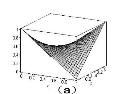
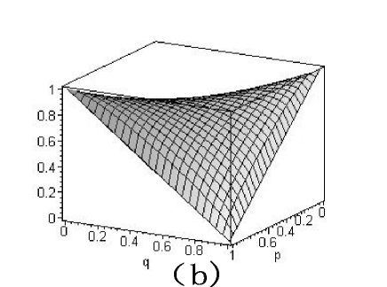
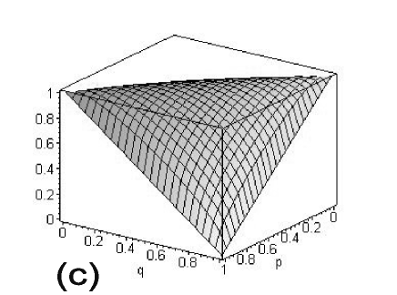
FIG. 1.: Player A’s payoff function versus $p$ and $q$ in 3-player cooperative via QSO strategy with initial state $c_{1}|000\rangle+c_{2}|111\rangle$. Parameter $a$ takes the following values: (a) $a=0$; (b)$a=0.33$; (c)$a=0.5$.

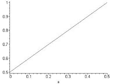
FIG. 2.: The maximum payoff for player A versus coefficient $a$ for 3-player game with QSO strategy with initial state $c_{1}|000\rangle+c_{2}|111\rangle$.

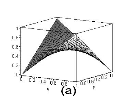
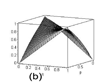
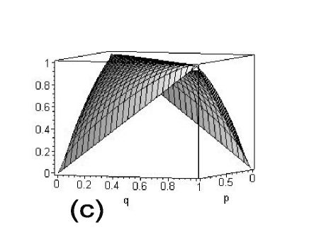
FIG. 3.: Player A’s payoff function versus $p$ and $q$ in 3-player cooperative via QSO strategy with initial state $c_{1}|001\rangle+c_{2}|110\rangle$. Parameter a takes the following values: (a) $a=0$; (b) $a=0.33$;(c)$a=0.5$.