Intermediate states in quantum cryptography and Bell inequalities

Abstract

Intermediate states are known from intercept/resend eavesdropping in the BB84 quantum cryptographic protocol. But they also play fundamental roles in the optimal eavesdropping strategy on BB84 and in the CHSH inequality. We generalize the intermediate states to arbitrary dimension and consider intercept/resend eavesdropping, optimal eavesdropping on the generalized BB84 protocol and present a generalized CHSH inequality for two entangled quNits based on these states.

1 Introduction

The quantum cryptographic protocol, known as the BB84 [1], was originally developed for qubits. In this protocol the legitimate users, Alice and Bob, both use the same two mutually unbiased bases $A$ and $A^{\prime}$. Alice use them for state preparation and Bob chooses between the two bases for his measurement. But an eavesdropper performing the simple intercept/resend eavesdropping, may chose to measure in what is known as the intermediate basis or the Breidbart basis [2]. In the case of qubits it is possible to form four intermediate states, which falls into two mutually unbiased bases. However the eavesdropper need only use one of these bases.

It turns out that it is not only in the simple intercept/resend eavesdropping that these intermediate states appear. Also in the optimal eavesdropping strategy [3, 4], which consists of the eavesdropper using the optimal cloning machine, these states enters. In this case, they appear at the point where Bob and the eavesdropper, Eve, have the same amount of information, i.e. where their information lines cross. At this point their mixed states may be decomposed into a mixture of some of the intermediate states.

That the intermediate states also appear in the optimal eavesdropping strategy, also explains a curious observation. Namely, that the amount of information obtained by the eavesdropper at the crossing point between the information lines using optimal eavesdropping, and the amount of information she obtains performing intercept/resend eavesdropping in the intermediate basis, is the same. However, the error rates are quite different.

Further more intermediate states reappear in the Clauser-Horne-Shimony-Holt (CHSH) inequality [5] for two entangled qubits. Where the maximal violation is obtained when on the first qubit the measurement settings correspond to the two mutually unbiased bases $A$ and $A^{\prime}$, and on the second qubit the two intermediate bases. Moreover when introducing the same kind of noise as the eavesdropper does in the optimal eavesdropping strategy, the Bell violation naturally decreases. But it is interesting to notice that for the critical disturbance where the classical limit is reached, Bob and Eve have the same amount of information, i.e. this happens at the crossing point of the information lines. This crossing point between the two information lines is a very important point, since upto this limit Alice and Bob can use the fact that they have more mutual information than the eavesdropper and they can create a secure key just by using classical error correction and one-way privacy amplification. Hence the CHSH inequality for qubits can be used as a security measure [6, 7].

In the three situation just described, intercept/resend eavesdropping, optimal eavesdropping and the CHSH-inequality, the intermediate states keep reappearing and seem to play a fundamental role.

A natural question to ask is ’what happens in higher dimensions?’. This is the question we try to answer, at least partially, here. It is possible to generalize the BB84 protocol to arbitrary dimension [8, 9, 10, 3, 4], simply by adding basis vectors to the two mutually unbiased bases, so that for $N$ dimension each basis contain $N$ vectors. The intermediate states may also be generalized to arbitrary dimensions. However, in higher dimensions they do in general not form bases. But it is possible to associate with each intermediate state a projector, which represents a binary measurement.

With the use of these generalized intermediate states we investigate intercept/resend eavesdropping, optimal eavesdropping and a generalized CHSH inequality in arbitrary dimension to see if they play the same role as in two dimension.

In section 2 we introduce the intermediate states for quNits. In section 3 we shortly discuss intercept/resend eavesdropping using the intermediate states. In section 4 we compare optimal eavesdropping with the intercept/resend eavesdropping strategy. Then in section 5 we present a generalized Bell inequality for two entangled quNits. In section 6 we consider the Bell violation as a function of the disturbance the optimal eavesdropping strategy would lead to. The last sections of the paper is devoted to a study of the inequality we have presented. In section 7 we discuss some features of the inequality by giving examples in three dimensions. Since recently the strength of a Bell inequality has been measured in terms of its resistance to noise we discuss this issue in section 8. Section 9 is devoted to a brief study of the required detection efficiency. Finally in section 10 we have conclusion and discussion.

2 The intermediate states

The quantum cryptographic protocol BB84 can easily be generalized to arbitrary dimension, this has already been discussed in the literature [8, 10]. The protocol works in exactly the same way as for qubits with the sole exception that for quNits each of the two mutually unbiased bases $A$ and $A^{\prime}$ used by Alice and Bob contain $N$ basis states instead of two. So that Alice sends at random (and with equal probability) one of the $2N$ possible states and Bob choses to measure in one of the two bases $A$ and $A^{\prime}$.

In this section we define the intermediate states between these two bases. The basis $A$ is chosen as the computational basis,

$$|\,{a}_{0}\,\rangle,\cdots,|\,{a}_{N-1}\,\rangle,$$ (1)

and the second basis, $A^{\prime}$, is the Fourier transform of the computational basis:

$$|\,{a}_{k}^{\prime}\,\rangle=\frac{1}{\sqrt{N}}\sum_{n=0}^{N-1}\exp\left(\right.\frac{2\pi i~{}kn}{N}\left.\right)|\,{a}_{n}\,\rangle$$ (2)

These two bases are mutually unbiased, i.e.

$$\langle\,{a}_{n}\,|\,{a}_{k}^{\prime}\,\rangle=\frac{\exp\left(\right.\frac{2\pi i~{}kn}{N}\left.\right)}{\sqrt{N}}$$ (3)

This means that the distance between pairs of state from the two bases is $\cos(\theta)=1/\sqrt{N}$.

Having two states, it is possible to define a state which lies exactly in between the two, which means that it has the same overlap with both states and it is the state closest to the two original states which has this property. The intermediate state are obtained by forming all possible pairs of the states from the two bases. They are shown in the table below:

	${a}_{0}^{\prime}$	${a}_{1}^{\prime}$	$\cdots$	${a}_{N-1}^{\prime}$
${a}_{0}$	${m}_{00}$	${m}_{01}$	$\cdot$	${m}_{0,N-1}$
${a}_{1}$	${m}_{10}$	${m}_{11}$	$\cdot$	${m}_{1,N-1}$
$\vdots$	$\cdot$	$\cdot$	$\cdot$	$\cdot$
${a}_{N-1}$	${m}_{N-1,0}$	${m}_{N-1,1}$	$\cdot$	${m}_{N-1,N-1}$

Explicitly the intermediate state between $|\,{a}_{n}\,\rangle$ and $|\,{a}_{k}^{\prime}\,\rangle$ is defined in the following way

$$|\,{m}_{nk}\,\rangle = \frac{1}{\sqrt{C}}\left[\exp\left(\frac{2\pi i~{}kn}{N}\right)|\,{a}_{n}\,\rangle+|\,{a}_{k}^{\prime}\,\rangle\right]$$ (4)

where $C=2(1+1/\sqrt{N})$ is the normalization constant and the phase comes from the overlap between $|\,{a}_{n}\,\rangle$ and $|\,{a}_{k}^{\prime}\,\rangle$, see eq.(3). The index of the $m$-states are such that the first index always refers to the $A$ and the second to the $A^{\prime}$-basis. Since each basis contains $N$ states it is possible to form $N^{2}$ intermediate states, simply by forming all pairs of states from the two bases.

In general the intermediate state $|\,{m}_{\alpha\beta}\,\rangle$ between two arbitrary initial states $|\,\alpha\,\rangle$ and $|\,\beta\,\rangle$ is defined as

$$|\,{m}_{\alpha\beta}\,\rangle=\frac{\sqrt{\langle\,\alpha\,|\,\beta\,\rangle}|\,\alpha\,\rangle+\sqrt{\langle\,\beta\,|\,\alpha\,\rangle}|\,\beta\,\rangle}{\sqrt{2}\sqrt{|{\langle\,\alpha\,|\,\beta\,\rangle}|+|{\langle\,\alpha\,|\,\beta\,\rangle}|^{2}}}$$ (5)

The intermediate states may be defined in complete generality for arbitrary initial states and any number of them. In this case the intermediate state is found by forming the mixture of all the initial states with equal weight, the eigenstate state with the largest eigenvalue of this mixture corresponds to the intermediate state. Naturally these definitions are equivalent and lead to the same intermediate state.

Considering the intermediate states leads to the following conditional probabilities

$$p({{m}_{nk}}|{{a}_{n}})=p({{m}_{nk}}|{{a}_{k}^{\prime}})=\frac{1+\frac{1}{\sqrt{N}}}{2}\equiv F$$ (6)

Notice that this definition indeed recover the formula for cosine of half the angle: $\cos(\theta/2)=\sqrt{\frac{1+cos(\theta)}{2}}$. This is why the states have been named intermediate states, since they indeed lie in between the the two original states.

Whereas the probability for making an error is

$$p({{m}_{nk}}|{{a}_{q}})=p({{m}_{nk}}|{{a}_{p}^{\prime}})=\frac{1-\frac{1}{\sqrt{N}}}{2(N-1)}\equiv\frac{D}{N-1}$$ (7)

It is important to notice that the intermediates states in general not are orthogonal, indeed

$$\langle\,{m}_{kl}\,|\,{m}_{nm}\,\rangle = \frac{1}{\sqrt{N}C}\left[\sqrt{N}{\delta}_{kn}\exp\left({\frac{2\pi i}{N}(mn-lk)}\right)\right.$$ (8)

$$+ \left.\sqrt{N}{\delta}_{lm}+\exp\left({\frac{2\pi i}{N}(m-l)k}\right)+\exp\left({\frac{2\pi i}{N}(m-l)n}\right)\right]$$

This means that the generalized intermediate states do in general not form bases as in the two dimensional case. But they can still be used as binary measurements, this is discussed in the next section.

2.1 Intermediate states as binary measurements

It has just been shown that in general the intermediate states $|\,{m}_{kl}\,\rangle$ are not orthogonal, and hence they do not form bases as in the two dimensional case. It is however possible to use the corresponding projectors, $|\,{m}_{kl}\,\rangle\langle\,{m}_{kl}\,|$ as binary measurements.

Since the intermediate states are non-orthogonal, it means that the corresponding binary measurements are mutually incompatible. In other words, none of them can be measured together but they have to be measured one by one. A binary measurement, has as the name indicates two possible outcomes, 0 and 1. Where the zero outcome is interpreted as ’I guess the state was not $|\,{m}_{kl}\,\rangle$’, and the ’1’ outcome is interpreted as ’I guess the state was $|\,{m}_{kl}\,\rangle$’. However, the answers are statistical, in the sense that there is a certain probability for making the wrong identification.

It should be mentioned that the $N^{2}$ intermediate states constitutes a generalized measurement namely a so called POVM. We have

$$\sum_{n,k=0}^{N-1}\frac{1}{N}|\,{m}_{nk}\,\rangle\langle\,{m}_{nk}\,|=\leavevmode\hbox{\small 1\kern-3.8pt\normalsize 1}$$ (9)

However, we do not make use of this in what follows.

3 Intercept/resend eavesdropping

Suppose that the eavesdropper, Eve, performs the simple intercept/resend eavesdropping. This means that she intercepts the particle send by Alice, performs a measurement and according to the result prepares a particle which she then sends to Bob. She may choose to measure in the same bases as Alice and Bob, but she may also choose to use the intermediate states. In higher dimensions where the intermediate states do not form bases, this strategy becomes a bit artificial. It is nevertheless interesting to consider it briefly.

In arbitrary dimension where the intermediate states corresponds to binary measurements, the intercept/resend strategy using these measurements may look like this: When ever Eve obtains a ’1’, which means she can make a good guess of the state, she prepares a new state and sends it to Bob. Whereas in the cases where she gets a ’0’, which means she is unable to make a good guess, she does not send anything to Bob. In this way we are only considering the cases where Eve does obtain a useful answer. This strategy, of course, gives rise to a huge amount of losses and errors on Bobs side, but it is however interesting to evaluate the amount of information that Eve obtains in this case, i.e. considering only the measurements where she gets a positive answer.

The probability of making the correct identification is given by eq.( 6) and is equal to $\frac{1}{2}+\frac{1}{2\sqrt{N}}$. Whereas the probability of wrong identification, i.e. of an error is given by eq.( 7) and is equal to $\frac{1}{(N-1)}(\frac{1}{2}-\frac{1}{2\sqrt{N}})$. This means that the (Shannon) information obtained by Eve is given by [10]

$${I}_{int,Eve}^{N} = \log_{2}(N)+\left(\frac{1}{2}+\frac{1}{2\sqrt{N}}\right)\log_{2}\left(\frac{1}{2}+\frac{1}{2\sqrt{N}}\right)$$ (10)

$$+ \left(\frac{1}{2}-\frac{1}{2\sqrt{N}}\right)\log_{2}\left(\frac{1}{(N-1)}\left(\frac{1}{2}-\frac{1}{2\sqrt{N}}\right)\right)$$

on the ’1’ outcomes of her measurements.

In the next section we will compare this amount of information to the amount of information obtained performing optimal eavesdropping at the point where the information lines between Bob and Eve cross.

4 The optimal cloning machine

The optimal eavesdropping strategy in any dimension, is believed to be given by a asymmetric version of the quantum cloning machine [11] which clones optimally the two mutually unbiased bases [4]. Using this cloner, Eve can obtain two copies of different fidelity of the state prepared by Alice. Usually Eve keeps the bad copy and sends the good one on to Bob. For a full description of how this eavesdropping strategy and of the cloning machine involved, see [4]. Here we are only concerned with the final state that Bob receives, which means how the optimal eavesdropping strategy influence the state obtained by Bob. In the case of no eavesdropping Bob receives the same pure state as was send by Alice. But in the case of eavesdropping Bob receives a mixed state.

Assume that without eavesdropping Bob would have found the state $|\,{a}_{n}\,\rangle$ if measuring in the computational basis. The question is what happens to $|\,{a}_{n}\,\rangle$ as a result of the eavesdropping? Or in other words, how does the cloning machine influence the state $|\,{a}_{n}\,\rangle$? We are only interested in the final mixed state Bob receives, and that may be written as

$$\rho_{B}=F_{B}|\,{a}_{n}\,\rangle\langle\,{a}_{n}\,|+\frac{D_{B}}{N-1}\sum_{j=0,~{}j\neq n}^{N-1}|\,{a}_{j}\,\rangle\langle\,{a}_{j}\,|$$ (11)

where $F_{B}$ is the fidelity and $D_{B}=1-F_{B}$ is the total disturbance. A similar expressing can be obtained for the $A^{\prime}$ basis states. As a result of the eavesdropping the amount of information that Bob gets is

$${I}_{opt,bob}^{N}=\log_{2}(N)+F_{B}\log_{2}(F_{B})+(1-F_{B})\log_{2}\left(\frac{1-F_{B}}{N-1}\right)$$ (12)

The optimal eavesdropping strategy is symmetric under the exchange of Bob and Eve. This means that the mixed state, ${\rho}_{E}$, which Eve obtains can be written on the same form as Bob’s mixed state, just with different coefficients, i.e.

$$\rho_{E}=F_{E}|\,{a}_{n}\,\rangle\langle\,{a}_{n}\,|+\frac{D_{E}}{N-1}\sum_{j=0,~{}j\neq n}^{N-1}|\,{a}_{j}\,\rangle\langle\,{a}_{j}\,|$$ (13)

And equivalently the amount of information obtained by Eve is given by

$${I}_{opt,eve}^{N}=\log_{2}(N)+F_{E}\log_{2}(F_{E})+(1-F_{E})\log_{2}\left(\frac{1-F_{E}}{N-1}\right)$$ (14)

It is interesting and important to consider the point where the information lines between Bob and Eve cross. Since when Alice and Bob share more information that Alice and Eve, Alice and Bob can use one-way privacy amplification to obtain a secret key. Using the explicit form and coefficients of the cloning machine it is possible to show (this was done in [4]) that the information curves cross at the point where

$$F_{B}=F_{E}=F=\frac{1}{2}+\frac{1}{2\sqrt{N}}$$ (15)

$$D_{B}=D_{E}=D=\frac{1}{2}-\frac{1}{2\sqrt{N}}$$ (16)

This is exactly the same fidelity (or probability of guessing correctly the state) that Eve obtained using the intercept/resend eavesdropping using the intermediate states. Which means that we have just shown that

$$I_{Int,eve}^{N}={I}_{opt,eve}^{N}({\rm crossing~{}point})$$ (17)

This is explained by the fact that, at the crossing point of the information lines, Eve’s mixed state can be decomposed into a mixture of some of the intermediate states, namely

$$\rho_{E}^{cross}=\frac{1}{N}\sum_{j=0}^{N-1}|\,{m}_{nj}\,\rangle\langle\,{m}_{nj}\,|$$ (18)

where again it has been assumed that $|\,a_{n}\,\rangle$ was the correct state. The same result holds for Bob, since at the crossing point Bob and Eve posses the same mixed state.

The mixture of the intermediate states may be interpreted as if Eve with probability $1/N$ has the state $|\,{m}_{nj}\,\rangle$ (there are N possible values of $j$). Eve, naturally, waits and performs her measurement after Alice has revealed in which basis the quNit was originally prepared. Then she measures her quNit in the same basis, which means that she uses either the basis $A$ or $A^{\prime}$.

Which means that the situation is the following: For the optimal eavesdropping strategy, Eve posses one of the intermediate states and she measures in one of the corresponding basis $A$ or $A^{\prime}$. Whereas in the intercept/resent eavesdropping with the intermediate states, the situation is exactly the opposite namely, Eve has one of the basis states from $A$ or $A^{\prime}$ and she measures the intermediate states. The two situations obviously lead to the same probabilities and hence the same amount of information.

5 The Bell inequality in arbitrary dimension

Recently there has been a big interest in generalizing various type of Bell inequalities [12], [13]-[18] in higher dimension. The Bell inequality we present here [19] makes use of the intermediate states, in a way similar to the CHSH inequality. This means that first we present the measurements and the quantum limit and only afterwards the local variable bound. So at first we just write down a particular sum of joint probabilities.

5.1 The Bell inequality: The quantum mechanical limit

Suppose that Alice and Bob share many maximally entangled state of two quNits. In the computational basis this state may be written as

$$|\,\psi\,\rangle=\frac{1}{\sqrt{N}}\sum_{i=0}^{N-1}|\,a_{i},a_{i}\,\rangle$$ (19)

For each of her quNits Alice has the choice of two measurements, namely to measure the basis $A$ or the basis $A^{\prime}$. Whereas Bob for each of his quNits has the choice between $N^{2}$ binary measurements, corresponding to all the intermediate states of the two bases used by Alice.

In order to write down the Bell inequality, it is convenient to assign values to the various states. In the table below is shown the values:

value	$A$	$A^{\prime}$	$M_{0}$	$M_{1}$	$\cdots$	$M_{N-1}$
0	$|\,a_{0}\,\rangle$	$|\,{a_{0}}^{\prime}\,\rangle$	$|\,m_{00}\,\rangle$	$|\,m_{01}\,\rangle$	$\cdots$	$|\,m_{0,N-1}\,\rangle$
1	$|\,a_{1}\,\rangle$	$|\,{a_{1}}^{\prime}\,\rangle$	$|\,m_{11}\,\rangle$	$|\,m_{12}\,\rangle$	$\cdots$	$|\,m_{10}\,\rangle$
$\cdots$	$\cdots$	$\cdots$	$\cdots$	$\cdots$	$\cdots$	$\cdots$
$N-1$	$|\,a_{N-1}\,\rangle$	$|\,{a_{N-1}}^{\prime}\,\rangle$	$|\,m_{N-1,N-1}\,\rangle$	$|\,m_{N-1,0}\,\rangle$	$\cdots$	$|\,m_{N-1,N-2}\,\rangle$

Notice that intermediate states have been organized into $N$ sets so that the value of the state is always given by the first index. Moreover this organization into the sets $M_{0},\ldots,M_{N-1}$, simplifies the notation in what follows. However, it is important to remember that the states in each of the sets are not orthogonal, in other words they do not form $N$ orthogonal bases.

The inequality is a sum of joint probabilities. And it is obtained by summing all the probabilities for when the results of the measurements are correlated and from this sum subtract all the probabilities when the results are not correlated, i.e.

$$B_{N} = \sum p(\rm{results~{}correlated})$$

$$- \sum p(\rm{results~{}not~{}correlated})$$

Suppose that Alice measures in the $A$ basis and Bob measures the projectors in the set $M_{0}$. For this combination of measurements, there are the following contributions to the sum $B_{N}$:

$$P(M_{0}=A) = \sum_{i=0}^{N-1}p(m_{ii}\bigcap a_{i})=\frac{1}{2}+\frac{1}{2\sqrt{N}}$$ (20)

$$P(M_{0}\neq A) = \sum_{i,j=0,j\neq i}^{N-1}p(m_{ii}\bigcap a_{j})=\frac{1}{2}-\frac{1}{2\sqrt{N}}$$ (21)

Where $P(M_{0}=A)$ should be read as follows: Bob measures one of the projectors in $M_{0}$ and Alice measures $A$, and Bob obtains the value which is correlated with Alice’s result. On the other hand $P(M_{0}\neq A)$ means that Bob’s result is not correlated with the result obtained by Alice. The probability $p(m_{kl}\bigcap a_{n})=p(m_{kl}|a_{n})p(a_{n})$ is the joint probability for obtaining both $|\,a_{n}\,\rangle$ and $|\,m_{kl}\,\rangle$.

The same is the case if Bob measures the projectors in any of the other sets $M_{1},\ldots,M_{N-1}$ and Alice always measures in $A$. And again if Bob uses $M_{0}$ and Alice $A^{\prime}$. Which means we have $P(M_{i}=A)=P(M_{0}=A^{\prime})=\frac{1}{2}+\frac{1}{2\sqrt{N}}$ and $P(M_{i}\neq A)=P(M_{0}\neq A^{\prime})=\frac{1}{2}-\frac{1}{2\sqrt{N}}$.

Now consider the case where Bob uses $M_{1}$ and Alice $A^{\prime}$, in this case Bob consistently finds a value which is $N-1$ higher than the value which correlates him with Alice. To see this, assume for example that Bob has the state $|\,a_{0}^{\prime}\,\rangle$ which is assigned the value $0$. But the state in $M_{1}$ which gives the correct identification of this state is $|\,m_{N-1,0}\,\rangle$, but this state has been assigned the value $N-1$. Similar for all the other states, which leads to $P(M_{1}=A^{\prime}+(N-1))=\frac{1}{2}+\frac{1}{2\sqrt{N}}$ and $P(M_{1}\neq A^{\prime}+(N-1))=\frac{1}{2}-\frac{1}{2\sqrt{N}}$. Actually, when ever Alice measures $A^{\prime}$ and Bob uses any of the $M_{i}$, Bob consistently finds a value which is $N-i$ higher than the one which correlates him with Alice. This means that $P(M_{i}=A^{\prime}+(N-i))=\frac{1}{2}+\frac{1}{2\sqrt{N}}$ and $P(M_{i}\neq A^{\prime}+(N-i))=\frac{1}{2}-\frac{1}{2\sqrt{N}}$.

It is now possible to write and evaluate the sum $B_{N}$

$$B_{N} = \sum_{i=0}^{N-1}P(M_{i}=A)-\sum_{i=0}^{N-1}P(M_{i}\neq A)$$ (22)

$$+\sum_{i=0}^{N-1}P(M_{i}=A^{\prime}+(N-i))-\sum_{i=0}^{N-1}P(M_{i}\neq A^{\prime}+(N-i))$$

$$= 2N\left(\left(\frac{1}{2}+\frac{1}{2\sqrt{N}}\right)-\left(\frac{1}{2}-\frac{1}{2\sqrt{N}}\right)\right)$$

$$= 2\sqrt{N}$$

The quantity $B_{N}$ is a sum of $2N\times N^{2}$ terms if written out explicitly. In the next section we show that a local variable model which tries to attribute definite values to the observables will reach a maximum value of 2. This shows that we have obtained a Bell inequality where the quantum violation grows with the squareroot of $N$.

5.2 The Bell inequality: the local variable limit

On Alice’s side $a_{0},\ldots,a_{N-1}$ are measured simultaneously in a single measurement as the basis $A$, which means that only one of them can come out true in a local variable model. The same is the case for ${a}_{0}^{\prime},\ldots,{a}_{N-1}^{\prime}$ which is measured as the basis $A^{\prime}$. This means that, for example, if $a_{i}$ is true, meaning that the measurement of $A$ will result in the outcome $a_{i}$, then all probabilities involving $a_{j}$ with $j\neq i$ must be zero. It is different on Bob’s side where each $m_{kl}$ is measured independently and hence they may all be true at the same time in a local variable model.

Assume now that according to some local variable model $a_{i}$ and ${a}_{j}^{\prime}$ are true. At the same time, in principle, all the $m_{kl}$ could be true too. But notice now that the only $m$-state which will give a positive contribution to the quantity $B_{N}$ is the one which identifies both $a_{i}$ and ${a}_{j}^{\prime}$ correctly, i.e. $m_{ij}$. This will give rise to a contribution of $+2$. Whereas $m_{il}$ and $m_{kj}$ where only one index is correct, will only identify of the states correctly and the other one wrong. This means that these states, since this gives rise to one correct and one wrong identification, will result in a zero contribution. And finally the states $m_{kl}$ where both indices are wrong will only give rise to errors and will hence give a negative contribution of $-2$ to the sum $B_{N}$. Which means that

$$B_{N}\leq 2$$ (23)

However, we have already shown that quantum mechanically it is possible to violate this limit. Quantum mechanically the limit is $2\sqrt{N}$. This means that we have obtained a Bell inequality where the violation increases with the squareroot of the dimension.

For N=3, the inequality has been checked in various ways numerically. First of all it has been checked that $2\sqrt{3}$ is indeed the quantum mechanical limit to this sum of probabilities and that this maximum is reached for the maximally entangled state. Moreover, it has been checked using ”polytope software” [13, 20] that the inequality eq.(23) is optimal for the measurement settings which we have presented here.

6 Bell parameter as a function of $\rho_{B}$

In this section we investigate how the Bell violation decreases as a function of the disturbance introduced by the eavesdropper. It is not necessary to think of it in terms of quantum cryptography and eavesdropping, but simply that the quantum channel from Alice to Bob is noisy and that the noise which is introduced is identical to the noise an eavesdropper using the optimal cloning machine would introduce.

Assume, without loss of generality, that without disturbance, Bob would have received the state $|\,a_{0}\,\rangle$, then we know that the mixed state that he obtains as a function of the disturbance can be written eq.(11)

$$\rho_{B}=F_{B}|\,{a}_{0}\,\rangle\langle\,{a}_{0}\,|+\frac{D_{B}}{N-1}\sum_{i=1}^{N-1}|\,{a}_{i}\,\rangle\langle\,{a}_{i}\,|$$

In order to compute $S(\rho_{B})$ it is enough to consider the case where Bob for example use the states in $M_{0}$ for his measurements, the rest of the terms in the inequality follows by symmetry.

All the states in the $M_{0}$ set are of the form $|\,m_{jj}\,\rangle$. First computing the various probabilities $\langle\,m_{jj}\,|\rho_{B}|\,m_{jj}\,\rangle$, we find

$$\langle\,m_{jj}\,|\rho_{B}|\,m_{jj}\,\rangle = F_{B}\overbrace{\langle\,m_{jj}\,|\,a_{0}\,\rangle\langle\,a_{0}\,|\,m_{jj}\,\rangle}^{p(m_{jj}|a_{0})}$$ (24)

$$+ \frac{D_{B}}{N-1}\sum_{i=1}^{N-1}\underbrace{\langle\,m_{jj}\,|\,a_{i}\,\rangle\langle\,a_{i}\,|\,m_{jj}\,\rangle}_{p(m_{jj}|a_{i})}$$

There are two different cases which have to be checked independently, namely $j=0$ and $j\neq 0$: For $j=0$ we have

$$\langle\,m_{00}\,|\rho_{B}|\,m_{00}\,\rangle=F_{B}F+(N-1)\frac{D_{B}}{N-1}\frac{D}{N-1}$$ (25)

and for $j\neq 0$ we have

$${\langle\,m_{jj}\,|\rho_{B}|\,m_{jj}\,\rangle}_{j\neq 0}=F_{B}\frac{D}{N-1}+F\frac{D_{B}}{N-1}+(N-2)\frac{D_{B}}{N-1}\frac{D}{N-1}$$ (26)

Where we have used that $p(m_{00}|a_{0})=F$ and $p{(m_{jj}|a_{0})}_{j\neq 0}=\frac{D}{N-1}$, see eq.(6) and eq.(7).

In the inequality $\langle\,m_{00}\,|\rho_{B}|\,m_{00}\,\rangle$ appears with a plus sign, since this is the probability of correctly identifying the state. At the same time ${\langle\,m_{jj}\,|\rho_{B}|\,m_{jj}\,\rangle}_{j\neq 0}$ appears $N-1$ times with a minus sign in the inequality, since these correspond to all the possible errors. This means that we can define

$$s(\rho) = \langle\,m_{00}\,|\rho_{B}|\,m_{00}\,\rangle-(N-1){\langle\,m_{jj}\,|\rho_{B}|\,m_{jj}\,\rangle}_{j\neq 0}$$ (27)

$$= F_{B}(F-D)-FD_{B}-\frac{N-3}{N-1}DD_{B}$$

There are $2N^{2}$ terms equal to $s(\rho_{B})$ in the Bell inequality, since there are $N^{2}$ intermediate states and each of them appear twice (once for each basis $A$ and $A^{\prime}$). On the other hand in each basis $A$ and $A^{\prime}$ each state appears with a probability $1/N$, this mean that the total Bell parameter is equal to

$$S(\rho_{B})=2Ns(\rho_{B})=2N\left(F_{B}(F-D)-FD_{B}-\frac{N-3}{N-1}DD_{B}\right)$$ (28)

It is now possible to answer a very interesting question, namely for which disturbance is $S(\rho_{B})=2$. Using the values of $F$ eq.(6) and $D$ eq.(7) and expressing $F_{B}=1-D_{B}$, one find that $S(\rho_{B})=2$ for

$$D_{B}^{S=2}=\frac{N^{\frac{3}{2}}-\sqrt{N}-N+1}{N^{\frac{3}{2}}+N^{2}-2N}$$ (29)

This can be compared to the disturbance $D$ at the crossing point between the information lines, this is shown in figure 1. We find that it is only for $N=2$ that $D_{B}^{S=2}=D$, and hence only in two dimension that the inequality we have presented here can be used as a security measure in quantum cryptography. However, it should be stressed that the violation of the inequality stops before the crossing point is reached. So a violation of the inequality, in any dimension, still means that Alice and Bob are within the secure zone.

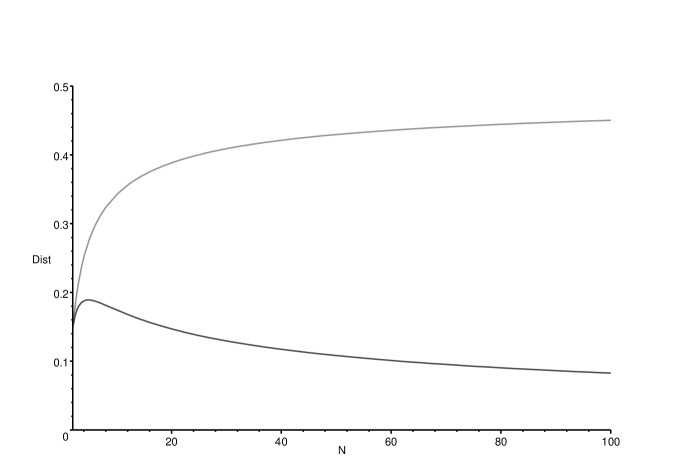
Figure 1: This figure shows as a function of the dimension, the disturbance at the crossing point $D$ (upper curve), and the disturbance for which the Bell violation stops $D^{S=2}$ (lower curve)

7 Interesting features of the $B_{3}$ inequality

In this section we restrict ourself to three dimension in order to show in a simple way some interesting properties of the inequality.

7.1 Complex versus real numbers

The first is related to the use of complex numbers. In the CHSH inequality for qubits, the maximal violation may be obtained by using real numbers only. Also the CGLMP inequality [18] show no difference between real and complex numbers. Here we show that if restricted to real numbers it is not possible to obtain maximal violation for the inequality we have presented.

Numerically we have found the settings which leads to the largest violation when restricted to real numbers. On Alice’s side the first basis is again the computational basis $A$, whereas the second basis $A^{r}$ (r stands for real) is found by making a $\pi/3$ rotation around the $(1,1,1)$ axis in $\Re^{3}$ and is explicitly given by

$$|\,{a}_{0}^{r}\,\rangle=\frac{1}{3}(2|\,{a}_{0}\,\rangle+2|\,{a}_{1}\,\rangle-1|\,{a}_{0}\,\rangle)$$

$$|\,{a}_{1}^{r}\,\rangle=\frac{1}{3}(-1|\,{a}_{0}\,\rangle+2|\,{a}_{1}\,\rangle+2|\,{a}_{0}\,\rangle)$$ (30)

$$|\,{a}_{2}^{r}\,\rangle=\frac{1}{3}(2|\,{a}_{0}\,\rangle-1|\,{a}_{1}\,\rangle+2|\,{a}_{0}\,\rangle)$$

The intermediate states are defined in the same way, and the three sets $M_{0}$, $M_{1}$ and $M_{2}$ again consists of nonorthogonal states. We find the following probabilities:

$$P(M_{0}=A)=5/6~{}~{}~{}~{} ~{}~{}~{}~{}P(M_{0}\neq A)=1/6$$ ,

$$P(M_{1}=A)=4/6~{}~{}~{}~{} ~{}~{}~{}~{}P(M_{1}\neq A)=2/6$$ ,

$$P(M_{2}=A)=5/6~{}~{}~{}~{} ~{}~{}~{}~{}P(M_{2}\neq A)=1/6$$ ,

$$P(M_{0}=A^{r})=5/6~{}~{}~{}~{} ~{}~{}~{}~{}P(M_{0}\neq A^{r})=1/6$$ ,

$$P(M_{1}=A^{r}+2)=4/6~{}~{}~{}~{} ~{}~{}~{}~{}P(M_{1}\neq A^{r}+2)=2/6$$ ,

$$P(M_{2}=A^{r}+1)=5/6~{}~{}~{}~{} ~{}~{}~{}~{}P(M_{2}\neq A^{r}+1)=1/6$$ ,

Alice and Bob are still assumed to share the maximally entangled state $|\,\psi\,\rangle$. Inserting these probabilities in the $B_{3}$ inequality leads to $B_{3}=10/3\approx 3.333$, which is smaller than the maximal violation which is $2\sqrt{3}\approx 3.464$.

The explanation for this difference can be found in the fact that the inequality $B_{N}$ has been optimized for mutually unbiased bases. In two dimension it is possible to have two such bases, for example the $z$ and the $x-$basis are mutually unbiased and both real. But when going to higher dimension it is not the case, for example in three dimension it is not possible to have two mutually unbiased bases and have them both real. Which means that in order to reach the maximum value, for the inequality we have presented here, it is necessary to introduce complex numbers. Whereas the CGLMP inequality for qutrits has not been optimized for mutually unbiased bases, this explains why it does not require complex numbers.

7.2 Binary measurements versus basis measurements

The $B_{N}$ inequality is on Bob’s side optimized for the $N^{2}$ binary measurements corresponding to the intermediate states of the two bases chosen by Alice. However it is possible to impose the additional requirement that not only must the measurements chosen by Bob maximize the probabilities, but they must also form basis. In other words it is possible to require that the $M$-sets correspond to orthogonal bases $M^{b}$ (b refers to basis). We have considered this question in three dimensions.

The $M^{b}$-basis which provide the optimal solution are defined in the following way: For the two mutually unbiased bases chosen by Alice there exist unitary operators $U_{i}$ such that

$$U|\,{a}_{i}\,\rangle=|\,{a}_{i}^{\prime}\,\rangle~{}~{}~{},~{}~{}~{}U=A^{\prime}\cdot A^{-1}$$ (31)

In this way the intermediate basis is defined as

$$|\,{m}_{ii}^{b}\,\rangle=\sqrt{U}|\,{a}_{i}\,\rangle~{}~{}~{},~{}~{}~{}M_{i}=\sqrt{U}A$$ (32)

Since $U$ is unitary $\sqrt{U}$ is well defined. It is possible to construct all three basis $M_{0}^{b}$, $M_{1}^{b}$ and $M_{2}^{b}$ in this way, choosing the unitary operator such that it transform the states in $A$ into any of the states in $A^{\prime}$. This definition leads to the following probabilities

$$P({M}_{0}^{b}=A)=7/9~{}~{}~{}~{} ~{}~{}~{}~{}P({M}_{0}^{b}\neq A)=2/9$$ ,

$$P({M}_{1}^{b}=A)=7/9~{}~{}~{}~{} ~{}~{}~{}~{}P({M}_{1}^{b}\neq A)=2/9$$ ,

$$P({M}_{2}^{b}=A)=7/9~{}~{}~{}~{} ~{}~{}~{}~{}P({M}_{2}^{b}\neq A)=2/9$$ ,

$$P({M}_{0}^{b}=A^{\prime})=7/9~{}~{}~{}~{} ~{}~{}~{}~{}P({M}_{0}^{b}\neq A^{\prime})=2/9$$ ,

$$P({M}_{1}^{b}=A^{\prime}+2)=7/9~{}~{}~{}~{} ~{}~{}~{}~{}P({M}_{1}^{b}\neq A^{\prime}+2)=2/9$$ ,

$$P({M}_{2}^{b}=A^{\prime}+1)=7/9~{}~{}~{}~{} ~{}~{}~{}~{}P({M}_{2}^{b}\neq A^{\prime}+1)=2/9$$ ,

These probabilities may again be used in the $B_{3}$ inequality. But it is important to realize that evenif the notation for the inequality is the same, the interpretation is different. Since the states in the ${M}_{i}^{b}$-sets are orthogonal and ${M}_{i}^{b}$ are bases, Bob no longer chooses between $9$ different binary measurements but between three basis measurements. However, it is possible to check that the local variable limit is not changed, i.e. it is still $2$. Inserting the above probabilities leads to ${B}_{3}^{b}=6(7/9-2/9)=10/3\approx 3.333$.

However, using basis measurements on Bob’s side leads to some other interesting results. It turns out that it is possible to reduce the number of terms in the inequality. The $B_{3}$ inequality is the sum of all correct guesses, subtracting all the errors. Using the intermediate bases ${M}_{i}^{b}$ it is possible to subtract only half of the errors and in this way obtain a different inequality with a different local variable limit, namely $S_{12}\leq 3$,

$$S_{12} = P({M}_{0}^{b}=A)+P({M}_{1}^{b}=A)+P({M}_{2}^{b}=A)$$ (33)

$$+ P({M}_{0}^{b}=A^{\prime})+P({M}_{1}^{b}=A^{\prime}+2)+P({M}_{2}^{b}=A^{\prime}+1)$$

$$- P({M}_{0}^{b}=A+1)-P({M}_{1}^{b}=A+1)-P({M}_{2}^{b}=A+1)$$

$$- P({M}_{0}^{b}=A^{\prime}+2)-P({M}_{1}^{b}=A^{\prime}+1)-P({M}_{2}^{b}=A^{\prime})$$

$$\leq 3$$

Inserting the above probabilities leads to the quantum mechanical maximum for this inequality namely, $S_{12}=6(7/9-1/9)=4$.

8 Resistance to noise

In the recent papers on Bell inequalities, the strength of the inequality has been measured in terms of its resistance to noise [16, 17, 18]. The question is how much noise can be added to the maximally entangled state, $|\,\psi\,\rangle$, and still obtain the Bell violation. The more noise which can be added to the system the better, since this means that the inequality is robust against noise.

What is meant by noise naturally has to be specified. In the previous section we, for example, considered the noise which is introduced by an eavesdropper when she uses the optimally eavesdropping strategy. However, the noise which was until recently used in the measure of the strength of an inequality was uncolored noise. This means that the maximally entangled state is mixed with the maximally mixed state, so that the quantum state becomes

$$\rho_{mix}=\lambda_{mix}|\,\psi\,\rangle\langle\,\psi\,|+(1-\lambda_{mix})\frac{\leavevmode\hbox{\small 1\kern-3.8pt\normalsize 1}}{N^{2}}$$ (34)

This can be interpreted as if Bob with probability $\lambda_{mix}$ receives the maximally entangled state and with probability $1-\lambda_{mix}$ he receives the maximally mixed state. For the maximally entangled state the Bell inequality, $B_{N}$ (23) has maximal violation, i.e. $S=2\sqrt{N}$. Whereas for the maximally mixed state each of the probabilities in the inequality is equal to $1/N$, hence $S(\leavevmode\hbox{\small 1\kern-3.8pt\normalsize 1}/N^{2})=2(2-N)$. This leads to

$$S(\rho_{mix})=2~{}~{}~{}\Longleftrightarrow~{}~{}~{}\lambda_{mix}^{B_{N}}=\frac{N-1}{N+\sqrt{N}-2}$$ (35)

For $N=3$, this is $\lambda_{mix}^{B_{3}}=\frac{2}{1+\sqrt{3}}\simeq 0.73$. In comparison, the CGLMP inequality is more robust to this kind of noise, since they find a violation until $\lambda_{mix}^{CGLMP}\simeq 0.69$.

Recently it has been argued that the use of uncolored noise in this measure lead to problems [21, 22]. At the same time a different kind of noise was introduced, namely to mix the maximally entangled state with the closest separable state, i.e.

$$\rho_{cs}=\lambda_{sep}|\,\psi\,\rangle\langle\,\psi\,|+(1-\lambda_{sep})\rho_{sep}$$ (36)

where $\rho_{sep}=\frac{1}{N}\sum_{i=0}^{N-1}|\,a_{i},a_{i}\,\rangle\langle\,a_{i},a_{i}\,|$ [23]. Examining what happens to the Bell violation when introducing the state $\rho_{sep}$ in $B_{N}$ eq.(23), shows that when Alice measures in the $A$ basis, Alice and Bob remain perfectly correlated - which means maximal violation of that part of the inequality concerning measurement combinations involving $A$. Whereas when Alice measures in the $A^{\prime}$ basis Bob is left with the maximally mixed state, which means that all the joint probabilities involving using $A^{\prime}$ on Alice’s side are equal to $1/N$. In total this leads to

$$S(\rho_{cs})=2~{}~{}~{}\Longleftrightarrow~{}~{}~{}\lambda_{sep}^{B_{N}}=\frac{N-\sqrt{N}}{N+\sqrt{N}-2}$$ (37)

which for $N=3$ is $\lambda_{sep}^{B_{3}}=\frac{3-\sqrt{3}}{1+\sqrt{3}}\simeq 0.46$. Whereas the CGLMP inequality again has $\lambda_{sep}^{CGLMP}\simeq 0.69$. Which means that the inequality we have introduced here is much more robust to this kind of noise.

It should be stressed that the same measurement settings have been used in both evaluations of $\lambda$, and that the CGLMP inequality has been optimized to be resistant to the uncolored noise. It is nevertheless interesting to see how the robustness of the $B_{N}$ inequality change depending on the different noise added to the system.

9 Minimum detection efficiency

To conclude the study of the inequality (23), let us consider the minimum detection efficiency required to violate it. This question is interesting both from a fundamental point of view (the so called detector efficiency loophole [24]) and for the practical question: How to test a quantum device, like a quantum cryptography system? [25, 7]. For simplicity we assume that all detectors have the same efficiency $\eta$. The problem is what to do with the cases that only one detector fires. A natural possibility attributes the value zero to bob whenever his detector did not fire and a random value to Alice whenever her detector did not fire. In this way, if only Alice detects a quNit, the Bell function vanishes. Whereas, if only Bob detects, the Bell function is the same as for the maximally mixed state, i.e. $2(2-N)$ as in the previous section. Thus the inequality reads:

$$\frac{\eta^{2}\cdot 2\sqrt{N}+\eta(1-\eta)\cdot(0+2(2-N))}{\eta^{2}+2\eta(1-\eta)}\leq 2$$ (38)

From this inequality one finds the threshold efficiency:

$$\eta_{threshold}=\frac{N}{N+\sqrt{N}-1}$$ (39)

For qubits, i.e. N=2, one recovers the welknown threshold, usually derived from the Clauser-Horn inequality [26]: $\eta_{threshold}^{(N=2)}\approx 82.8\%$. This threshold is minimal and slightly better for N=4: $\eta_{threshold}^{(N=4)}=80\%$. For higher dimensions the threshold increases and tends to 1.

It would be interesting to investigate the behavior of non-maximally entangled states, since Eberhard found that for qubits the threshold then decreases [28]. Let us mention that recentyly S. Massar proved that there are inequalities for which the threshold tends to zero exponentially, at least for very large dimensions [27] and, with colleagues he investigated situation similar to the one studied in this section [29].

10 Conclusion

For qubits the intermediate states play fundamental roles in at least three different place: intercept/resend eavesdropping in the BB84 protocol for quantum cryptography, optimal eavesdropping also in the BB84 protocol and in the CHSH-inequality for two entangled qubits. The work we have presented here, is the result of a study, of the use of these intermediate state in the same situations but in arbitrary dimension.

In this paper we have first discussed the generalization of the intermediates states of two mutually unbiased bases, showing that these states are in general not orthogonal and hence do not form basis as in the case for qubits. We have also discussed how they, nevertheless, can be use as binary measurements. With these measurements we have considered the same situations as known from the qubit case.

We have considered eavesdropping in the generalized BB84 protocol (always considering only two bases). When the eavesdropper use the optimal eavesdropping strategy, her information increase as a function of the disturbance that she introduce and at the same time Bob’s information is a decreasing function of the disturbance. For a given disturbance their information lines cross. We have shown that the amount of information that the eavesdropper obtain at this crossing point, is exactly the same amount of information she would have obtained using the simple intercept/resend strategy using the intermediate states. However leading to a much higher disturbance. This is explained by the fact that in any dimension Eve’s mixed state can at the crossing point be decomposed into a sum of some of the intermediate states. Hence, in the optimal eavesdropping strategy, at the crossing point, Eve has one of the intermediate state but perform her measurement in the same basis as the state was originally prepared. Whereas in the intercept/resend strategy using the intermediate states as binary measurements, Eve has the state which was originally prepared by Alice, but measure one of the intermediate states. This means that the two situations are exactly opposite, and therefore lead to the same probabilities and hence the same information.

The maximal settings for the CHSH-inequality for qubits are two mutually unbiased bases on Alice’s side and using the intermediate states on Bob’s side. In the case of qubits the four intermediate states form two bases. This means that in this case both Alice and Bob have the choice of measuring one of two mutually unbiased bases.

In higher dimension where the intermediate states do not form bases, Bob instead use the corresponding projectors as binary measurements. Which means that he choose between $N^{2}$ mutually incompatible measurements, whereas Alice still choose between two basis measurements. The generalized inequality we present has the local variable limit equal to $2$ in any dimension whereas the maximal quantum mechanical value is $2\sqrt{N}$. In other words we find a violation which increase with the squareroot of the dimension. Due to the construction we also obtain the familiar CHSH-inequality for $N=2$.

It is known that the CHSH inequality may be used as a security measure in quantum cryptography for qubits. Since in this case a violation of the inequality is obtained until the disturbance introduced by the eavesdropper, reaches the disturbance at the crossing point of the information lines between Eve and Bob. Until this point Alice and Bob can use the fact that they share more mutual information than with Eve to obtain a secret key by means of one way privacy amplification. We have investigated the violation of the inequality we present here as a function for the disturbance introduced by the eavesdropper. We found that it is only for $N=2$ that the inequality can be used as a security measure, in the sense that in higher dimension the violation stops for a lower disturbance than the disturbance at the crossing point. This, however, does not mean that such an inequality does not exist, it only shows that the inequality which mimics the situation from two dimension is not the one which has this property in higher dimension.

On the other hand the inequality we have presented here may stand as a result by itself and as a Bell inequality in arbitrary dimension is has many nice properties. First of all, compared to the other inequalities which have been presented recently, this inequality gives maximal violation for maximally entangled states. This means this inequality may be used as a measure of entanglements. Moreover we have shown in examples in three dimensions that this inequality require complex numbers in order to have maximal violation. Restriction to the use of real numbers lead to a smaller violation. In comparison, the CHSH inequality for qubits and the CGLMP inequality for qutrits show no difference between using real or complex numbers. The explanation is due to the fact that the inequality we present here is optimized for mutually unbiased bases and in three dimension it is not possible to have two such bases without the use of complex numbers. Whereas in two dimension the $x$ and $z-$ bases are mutually unbiased and both real, and for the CGLMP inequality the explanation is that it is not optimized of mutually unbiased bases.

We have also shown that imposing the additional constrain that the $M$-sets actually form bases, leads to new inequalities. We have explicitly given an example in three dimensions, showing the optimal solution, for two basis measurements on Alice’s side and three basis measurements on Bob’s side.

The strength of a Bell inequality has been measured in terms of its resistance to noise. Until recently the noise was taken to be uncolored noise, which means that the maximally entangled state is mixed with the maximally mixed state. The inequality we present here is less resistant to this kind of noise that other inequalities which have been presented recently. It should however be mentioned that these inequalities have been optimized for this kind of noise. However, recently it was argued that using the uncolored noise leads to problems. At the same time a different kind of noise was introduced, namely mixing the maximally entangled state with the closest separable state. When using this measure we find that the inequality we present here, is much more robust than, for example, the CGLMP-inequality.

References

- [1] C. H. Bennett, G. Brassard, Proceedings of IEEE international Conference on Computers, Systems, and Signal Processing, Bangalore, India, December, 1984, pp. 175-179
- [2] See for example, C. Bennett, F. Bessette, G. Brassard, L. Salvail and J. Smolin, J. Cryptology (1992) 5:3-28
- [3] D. Bruss, C. Macchiavello, Phys. Rev. Lett. 88 127901 (2002)
- [4] N. Cerf, M. Bourennane, A. Karlsson, N. Gisin, Phys. Rev. Lett. 88 127902 (2002)
- [5] J. F. Clauser, M. A. Horne, A. Shimony, R. A. Holt, Phys. Rev. Lett 23 (1969) 880
- [6] C.A. Fuchs., N. Gisin, R.B. Griffiths, C.-S. Niu, and A. Peres, Phys. Rev. A 56, 1163-172, 1997.
- [7] N. Gisin, G. Ribordy, W. Tittel and H. Zbinden, Rev. Mod. Phys. 74, 145-195, 2002, Quant-ph/0101098.
- [8] H. Bechmann-Pasquinucci, W. Tittel, Phys. Rev. A 61, 062308 (2000)
- [9] H. Bechmann-Pasquinucci, A. Peres, Phys. Rev. Lett. 85, 3313 (2000)
- [10] M. Bourennane, A. Karlsson, G. Bjork, Phys. Rev. A 64, 052313 (2001)
- [11] N. J. Cerf, Phys. Rev. Lett. 84, 4497 (2000); J. Mod. Opt. 47, 187 (2000); Acta Phys. Slov. 48, 115 (1998).
- [12] J. S. Bell, Physics 1 (1964) 195
- [13] D. Kaszlikowski, P. Gnacinski, M Zukowski, W. Miklaszewski, A. Zeilinger, Phys. Rev. Lett 85, 4418 (2000)
- [14] T. Durt, D. Kaszlikowski, M. Zukowski, quant-ph/0101084
- [15] J.-L. Chen, D. Kaszlikowski, L. C. Kwek, M. Zukowski, C. H. Oh, quant-ph/0103099
- [16] D. Kaszlikowski, P. Gnacinski, M. Zukowski, W. Miklaszewski, A. Zeilinger, Phys. Rev. Lett. 85, 4418 (2000)
- [17] D. Kaszlikowski, L. C. Kwek, J.-L. Chen, M. Zukowski, C. H. Oh, quanth-ph/0106010
- [18] D. Collins, N. Gisin, N. Linden, S. Massar, S. Popescu, quant-ph/0106024
- [19] H. Bechmann-Pasquinucci, N. Gisin, quant-ph/0204122
- [20] R. M. Basoalto, I. Percival, quant-ph/0012024
- [21] D. Collins and S. Popescu, quant-ph/0106156, J. Phys. A, in press, 2002.
- [22] A. Acin, T. Durt, N. Gisin, J. I. Latorre, quant-ph/0111143 v 2, Phys. Rev. A, in press, 2002.
- [23] M. Plenio, V. Vedral, Phys. Rev. A 57 1619 (1998)
- [24] P. Pearle, Phys. Rev. D, 2, 1418, 1970; J.F. Clauser, M.A. Horne, A. Shimony, and R.A. Holt, Phys. Rev. Lett., 23, 880, (1969); E. Santos, Phys.Rev. A, 46, 3646, (1992).
- [25] D. Mayers and A. Yao, Proceedings of the 39th IEEE Conference on Foundations of Computer Science, 1998.
- [26] J. F. Clauser, and M. A. Horne, Phys. Rev. D 10, 526 (1974).
- [27] S. Massar, Phys. Rev. A 65 032121 (2002)
- [28] Ph.H. Eberhard, Phys. Rev. A 47, R747 (1993).
- [29] S. Massar, S. Pironio, J. Roland, B. Gisin, quant-ph/0205130