Trapping and cooling single atoms with far-off resonance intracavity doughnut modes

Abstract

We investigate cooling and trapping of single atoms inside an optical cavity using a quasi-resonant field and a far-off resonant mode of the Laguerre-Gauss type. The far-off resonant doughnut mode provides an efficient trapping in the case when it shifts the atomic internal ground and excited state in the same way, which is particularly useful for quantum information applications of cavity quantum electrodynamics (QED) systems. Long trapping times can be achieved, as shown by full 3-D simulations of the quasi-classical motion inside the resonator.

I Introduction

Cavity quantum electrodynamics (QED) is a powerful tool for the deterministic control of atom-photon interactions at the quantum level. In fact, the strong confinement allows to achieve the strong coupling regime where single quanta can profoundly affect the atom-cavity dynamics [1]. Many experiments have now reached this regime and interesting phenomena have been demonstrated, as a quantum phase gate [2], the Fock state generation in a cavity field [3], and quantum nondemolition detection of a single cavity photon [4]. Moreover, cavity QED offers unique advantages for quantum communication and quantum information processing applications. In fact, atoms may act as quantum memories, while photons are flexible transporters of quantum information, and quantum networks of multiple atom-cavity systems linked by optical interconnects have been already discussed in the literature [5]. The primary technical challenge on the road toward these applications is to trap individual neutral atoms within a high-finesse cavity for a reasonably long time. Recent experiments [6, 7] have already succeeded in trapping single atoms inside an optical cavity driven at the few photon level, just using the strong coupling with the cavity QED mode for both cooling and trapping. However, the scheme of Refs. [6, 7] is not entirely suitable for quantum communication purposes because it has limited operation flexibility and provides short trapping times (order of hundreds of microseconds). In fact, it employs a single cavity mode, while it is preferable to have an additional trapping mechanism which does not interfere with the cavity QED interactions able to provide the atom-photon entanglement needed for the manipulation of quantum information. With these respect, another experiment has already demonstrated significant trapping times ($\sim 28$ ms) of single Cs atoms within a cavity, employing an additional far-off resonance trapping (FORT) mode [8]. Using the fact that, in the strong coupling regime, the trajectory of an individual atom can be monitored in real time by the quasi-resonant cavity QED field [9], the FORT beam can be turned on as soon as the atom enters the cavity in order to increase its trapping time.

Several mechanisms for cooling inside an optical resonator have been already discussed in the literature [10, 11, 12, 13], involving either cavity mode driving, or direct atom driving via a classical laser field from the side, or even active feedback on atomic motion as in [14]. However, only the recent paper by van Enk et al. [15] has discussed in detail the effects of an additional FORT beam on the cooling and trapping dynamics and its interplay with the quasi-resonant cavity QED field. Here we shall consider a situation analogous to that of Ref. [15], even though we shall extend our study to new FORT mode configurations. We have chosen a parameter region corresponding to the weak driving limit, with an empty-cavity mean photon number $N_{e}\simeq 0.01$. We have performed full 3-D numerical simulations of the quasi-classical atomic motion, including the effects of spontaneous emission and dipole-force fluctuations.

In two-level systems, red-detuned FORT beams shift the atomic excited state $|e\rangle$ up and the ground state $|g\rangle$ down by the same quantity, and this is the most common situation, studied in great detail in [15]. However, the most interesting situation for quantum information processing applications is when both levels are shifted down by the FORT beam: in this case, excited and ground state atoms are trapped in the same position, and this greatly simplifies the quantum manipulation of the internal state. In fact, the most flexible situation for quantum information processing is having a trapping mechanism independent of the atomic internal state. This configuration can be realized by using a FORT that is red-detuned in such a way that the excited state is relatively closer to resonance with a higher-lying excited state than with the ground state. We shall discuss in detail both situations (equal or opposite optical Stark shifts), and we shall find the interesting result that in the case of equal Stark shifts for ground and excited state, the use of doughnut modes, that is, higher-order Gauss-Laguerre modes, as FORT mode, is able to increase significantly the trapping time within the cavity.

The paper is organized as follows. In Section II we describe the physics of an atom trapped in an optical potential and strongly interacting with a cavity QED field. We also discuss the changes introduced by the FORT doughnut mode. In Section III, applying the general approach developed in Ref. [16] to a cavity mode configuration, we discuss the conditions under which the center-of-mass motion of the atom can be adiabatically separated from the internal and cavity mode dynamics, and treated in a quasi-classical way. The corresponding 3-D Fokker-Planck equation for the phase-space atomic motion will be derived. In Section IV, the results of the numerical simulations of the corresponding stochastic differential equations will be presented in detail, and in Section V these results will be discussed for both equal and opposite energy shifts of the $|e\rangle$ and $|g\rangle$ states. Section VI is for concluding remarks.

II The physical problem

We consider a two level atom coupled to a quantized cavity mode and to an additional classical red-detuned FORT beam, coinciding with another longitudinal mode of the cavity, with a wavelength $\lambda_{S}$ longer than that of the quasi-resonant cavity mode, $\lambda_{g}$. The common situation is to consider lowest order Gaussian modes for both fields [15], having their maximum intensity along the cavity axis. Here we shall consider a different situation, where the FORT mode is a higher-order Gauss-Laguerre mode, the so-called doughnut mode, having its maximum intensity at a nonzero radial distance from the cavity axis. This means that the atoms are trapped out of the cavity axis (see Fig. 1 for a schematic description of the system). At first sight, this choice may look not optimal, because in this case the coupling with the fundamental Gaussian cavity QED field responsible for cooling is smaller. Nonetheless, we shall see that this choice is convenient in the case when the classical FORT mode shifts down both excited and ground state, which is the most interesting case for quantum information processing applications.

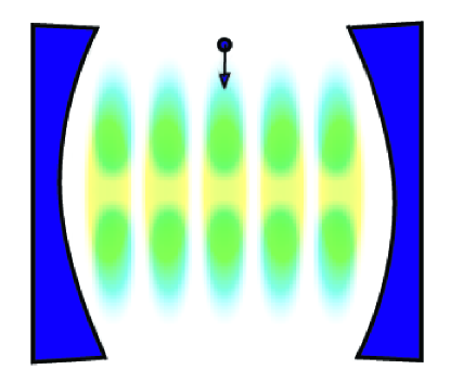
FIG. 1.: Schematic description of the system. Atoms falling from a magneto-optical trap are trapped within a cavity with a fundamental Gaussian quantized resonant mode (yellow) and an intense classical doughnut FORT mode (light blue).

We recall that the Laguerre-Gauss modes LG_pm are the solutions of the paraxial Helmoltz equation in cylindrical coordinates $(\rho,\vartheta,x$) [17]. In this paper we consider the doughnut modes with radial index $m\neq 0$ and azimuthal index $p=0$, whose intensity is given by

$$I_{0m}(\rho,x)=4P\frac{2^{m+1}}{\pi m!}\frac{\rho^{2m}}{W^{2(m+1)}(x)}\exp\left\{-\frac{2\rho^{2}}{W^{2}(x)}\right\}\sin^{2}(k_{S}x),$$ (1)

where $P$ is the power, $k_{S}=2\pi/\lambda_{S}$ the wavenumber, and $W(x)$ the beam radius. The doughnut mode radius is given by the position of the radial maximum, given by $\rho_{\max}=W(x)\sqrt{m/2}$. We can simplify the description assuming a nearly planar cavity, so that $W(x)\sim W_{S}$. The classical, red-detuned FORT mode induces AC Stark shifts $\Delta E_{g}$ on the ground state $|g\rangle$ and $\Delta E_{e}$ on the excited state $|e\rangle$ [18]. We can distinguish two different situations: (a) $|g\rangle$ is shifted down and $|e\rangle$ is shifted up, which happens in the common situation where only the $e\leftrightarrow g$ transition is close to the red detuned FORT mode. In this case the two shifts are opposite. (b) Both $|g\rangle$ and $|e\rangle$ are shifted down, which happens when $|e\rangle$ is closer to resonance with a higher-lying excited level than with the level $|g\rangle$ [19],[20],[21]. We shall study both situations and in case (b) we shall assume that the various detunings can be chosen so that the two levels are shifted down by the same quantity. Furthermore, to simplify the comparison between the two cases, we shall assume that the two situations occur with the same wavelength $\lambda_{S}$.

Considering a frame rotating at the probe driving frequency $\omega_{p}$, the Hamiltonian of the system can be written as

$$H=\frac{|\vec{P}|^{2}}{2M}+\hbar\omega_{ap}\sigma^{\dagger}\sigma+\hbar\omega_{gp}a^{\dagger}a+V(\vec{R})+\hbar\left(Ea^{\dagger}+E^{\ast}a\right),$$ (2)

where $\omega_{ap}=\omega_{eg}-\omega_{p}$ is the detuning of the the atomic resonance from the probe frequency, $\omega_{gp}=\omega_{g}-\omega_{p}$ is the detuning of the cavity QED mode with annihilation operator $a$, $\sigma=|g\rangle\langle e|$, $E$ is the cavity driving rate, and $\vec{R}$, $\vec{P}$ are the position and momentum vector operators of the atom, having a mass $M$. The interaction potential $V(\vec{R})$ describes the interaction between the internal atomic levels, the cavity modes and the atomic center-of-mass motion, and it is given by the coupling with the quantized cavity mode and with the FORT doughnut mode. Making the usual dipole and rotating wave approximations, this interaction term can be written

$$V(\vec{R})=\hbar g(\vec{R})\left(a^{\dagger}\sigma+\sigma^{\dagger}a\right)+V^{S}(\vec{R}),$$ (3)

where

$$g(\rho,x)=g_{0}\sin(k_{g}x)\exp\left\{-\frac{\rho^{2}}{W_{g}^{2}}\right\}$$ (4)

is the space-dependent Rabi frequency due to the coupling with the quantized mode, and the second term $V^{S}(\vec{R})$ describes the effect of the Stark shifts induced by the FORT mode, assuming the following form in the two cases, (a) and (b):

$$\text{case (a) \ \ \ }V^{S}(\vec{R}) = \hbar S(\vec{R})(\sigma^{\dagger}\sigma-\sigma\sigma^{\dagger})$$ (5)

$$\text{case (b) \ \ \ }V^{S}(\vec{R}) = -\hbar S(\vec{R}).$$ (6)

The frequency ac-Stark shift is generally given by $S(\rho,x)=\alpha I_{0m}(\rho,x)/4\hbar$ [22, 23], where $\alpha$ is the atomic polarizability and $I_{0m}(\rho,x)$ is the FORT intensity of Eq. (1), so that one can write

$$S(\rho,x)=S_{0}\rho^{2m}\sin^{2}(k_{S}x)\exp\left\{-\frac{2\rho^{2}}{W_{S}^{2}}\right\},$$ (7)

with $S_{0}=2^{m+1}P\alpha/\pi\hbar W_{S}^{2m+2}$. We have generally considered different waists $W_{g}$ and $W_{S}$ for the two modes, but they practically coincide in typical situations.

The FORT mode provides the main trapping mechanism. This means that the atom will be trapped around the anti-nodes of the red-detuned FORT field, because $S_{0}>g_{0}$ and the cavity QED field is weakly driven. However, due to the different wavelengths, one does not have a periodic situation, and the atom feels a different cavity QED coupling in different wells. In the experiment of Ref. [8] the cavity length $L$ is such that $2L=104\lambda_{g}=102\lambda_{S}$. To simplify our simulation we have however chosen $L=16\lambda_{g}=15\lambda_{S}$, as it has been done also in [15]. This is equivalent to choose a fictitious larger value for $\lambda_{S}$ which however does not modify the essential physics of the problem, because the FORT mode is in any case far-off resonance. With this choice we consider only $30$ potential wells in the cavity, only $8$ of which are quantitatively different (see Ref. [15]).

Dissipation, diffusion and all non-conservative effects appear due to spontaneous emission and cavity losses. The quantum evolution of the atom-cavity system is therefore described by a master-equation for the atom-cavity density operator $\rho$ [16]

$$\frac{d\rho}{dt} = -\frac{i}{\hbar}\left[H,\rho\right]+\kappa\left(2a\rho a^{\dagger}-a^{\dagger}a\rho-\rho a^{\dagger}a\right)-\gamma\left(\sigma^{\dagger}\sigma\rho+\rho\sigma^{\dagger}\sigma\right)$$ (8)

$$+ \frac{3\gamma}{4\pi}\int d^{2}\hat{k}~{}D(\hat{k}\cdot\hat{x})e^{-i\vec{k}\cdot\vec{R}}\sigma\rho\sigma^{\dagger}e^{i\vec{k}\cdot\vec{R}}$$ (9)

where $\kappa$ is the cavity damping rate and $\gamma$ is spontaneous emission decay rate. The last term describes the effects of atomic recoil, with $\hat{k}$ giving the direction of emitted photon and $D(\hat{k}\cdot\hat{x})=(1+(\hat{k}\cdot\hat{x})^{2})/2$ describing the angular pattern of dipole radiation [24].

III Quasi-classical description of the atomic motion

The internal and cavity dynamics is governed by the detunings, $\omega_{ap}$ and $\omega_{gp}$, the spontaneous emission rate $\gamma$, the driving rate $E$, the cavity damping rate $\kappa$, the FORT shift $S_{0}$, and the coupling constant $g_{0}$. In the parameter region relevant for current experiments, this dynamics is much faster than the atomic motional dynamics, especially for heavy atoms as Cs [8] or Rb [7]. Therefore, internal and cavity dynamics can be adiabatically eliminated in order to obtain a reduced effective evolution equation for the motional degrees of freedom only. This adiabatic elimination can be made in a systematic way by adapting the general approach developed for free space cooling situations in Ref. [16] to the present cavity scheme (see also [13]). One starts from the evolution equation of the Wigner operator obtained by performing the Wigner transform only on the motional Hilbert space, and writing this equation as a Taylor expansion in terms of two small parameters of the problem. Denoting with $k\simeq k_{g}\simeq k_{S}\simeq k_{a}=\omega_{eg}/c$ the typical wavenumber of the problem, we have that one small parameter is

$$\epsilon_{1}=\frac{\hbar k}{\Delta p}\ll 1,$$ (10)

showing that the motional state is characterized by a momentum spread $\Delta p$ much larger than the momentum kicks felt by the atom during any photon emission or absorption. The second small parameter is

$$\epsilon_{2}\simeq\frac{k\Delta p}{M\gamma}\simeq\frac{k\Delta p}{M\kappa}\ll 1,$$ (11)

which instead shows that the Doppler shift associated with the momentum spread is small with respect to the atomic and cavity linewidths. The two conditions set a lower and an upper bound for the momentum spread of the atom, which, thanks to the Heisenberg inequality, put also a lower and an upper bound for its position spread. These bounds allow to describe the atomic motion in classical terms, because the atom is sufficiently localized in phase space to make it possible to describe its motion in terms of trajectories, while at the same time the phase space spread always remains larger than $\hbar$ (see [9, 11]). The crucial point is that the two conditions (10) and 11) must be consistent and this happens when

$$\frac{\hbar^{2}k^{2}}{2M}\ll\hbar\gamma,\hbar\kappa.$$ (12)

This means supplementing the well known necessary condition for laser cooling in free space, $\hbar^{2}k^{2}/2M\ll\hbar\gamma$ (the atom has to be still in resonance after spontaneously emitting) [16], with an analogous condition for the exchange of cavity photons.

For small parameters $\epsilon_{1}$ and $\epsilon_{2}$, the atomic motion is much slower than the internal one, and the adiabatic elimination of the latter is obtained if the atomic kinetic energy term is neglected in the equation for the Wigner operator, which then effectively factorizes into a product of a stationary state $\eta\left(\vec{r}\right)$ for the cavity and internal degrees of freedom evaluated at the fixed atomic position $\vec{r}=(\rho,\theta,x)$, and a real-valued motional Wigner function $f(\vec{r},\vec{p},t)$. The stationary state $\eta\left(\vec{r}\right)$ satisfies the steady-state Bloch equation

$$L_{Bloch}(\vec{r})\eta(\vec{r}) \equiv -i\left[\omega_{ap}\sigma^{\dagger}\sigma+\omega_{gp}a^{\dagger}a+\left(Ea^{\dagger}+E^{\ast}a\right)+\frac{V(\vec{r})}{\hbar},\eta(\vec{r})\right]$$ (13)

$$+ \kappa\left(2a\eta(\vec{r})a^{\dagger}-a^{\dagger}a\eta(\vec{r})-\eta(\vec{r})a^{\dagger}a\right)$$ (14)

$$+ \gamma\left(2\sigma\eta(\vec{r})\sigma^{\dagger}-\sigma^{\dagger}\sigma\eta(\vec{r})-\eta(\vec{r})\sigma^{\dagger}\sigma\right)=0,$$ (15)

where $L_{Bloch}(\vec{r})$ comes from a zeroth-order expansion of the master equation (9) in the small parameters $\epsilon_{1}$ and $\epsilon_{2}$ of Eqs. (10) and (11).

The resulting equation for the Wigner function $f(\vec{r},\vec{p},t)$ is of Fokker-Planck type and is given by [13, 16]

$$\frac{\partial}{\partial t}f(\vec{r},\vec{p},t) = -\frac{\vec{p}}{M}\cdot\frac{\partial}{\partial\vec{r}}f(\vec{r},\vec{p},t)-\frac{\partial}{\partial\vec{p}}f(\vec{r},\vec{p},t)\cdot\vec{\phi}(\vec{r})$$ (16)

$$+ \hbar^{2}k_{a}^{2}\gamma\left\langle\sigma^{\dagger}\sigma\right\rangle(\vec{r})\sum_{i}E_{ii}\frac{\partial^{2}}{\partial p_{i}^{2}}f(\vec{r},\vec{p},t)+\sum_{ij}\eta_{ij}(\vec{r})\frac{\partial^{2}}{\partial p_{i}\partial r_{j}}f(\vec{r},\vec{p},t)$$ (17)

$$+ \sum_{ij}D_{ij}(\vec{r})\frac{\partial^{2}}{\partial p_{i}\partial p_{j}}f(\vec{r},\vec{p},t)+\sum_{ij}\Gamma_{ij}(\vec{r})\frac{\partial}{\partial p_{i}}(p_{j}f(\vec{r},\vec{p},t)).$$ (18)

All the coefficients of this Fokker-Planck equation depend upon average values and correlation functions of the internal and cavity degrees of freedom, evaluated on the stationary state at fixed atomic position $\eta\left(\vec{r}\right)$ of Eq. (15). An example is provided by the average value $\left\langle\sigma^{\dagger}\sigma\right\rangle(\vec{r})$ appearing in Eq. (18) in the diffusion term due to spontaneous emission, which also depends upon the diagonal matrix $E_{ii}$ given by $E_{xx}=2/5$, $E_{yy}=E_{zz}=3/10$ [13, 24]. The other atom-cavity quantities determining the Fokker-Planck equation coefficients are $\Phi\equiv a^{\dagger}\sigma+\sigma^{\dagger}a$ and $\Psi\equiv\sigma^{\dagger}\sigma-\sigma\sigma^{\dagger}$, whose expectation value determines the mean dipole force acting on the atom $\vec{\phi}(\vec{r})$. In fact,

$$\vec{\phi}(\vec{r})=\left\{\matrix{-\hbar\frac{\partial}{\partial\vec{r}}g(\vec{r})\left\langle\Phi\right\rangle(\vec{r})-\hbar\frac{\partial}{\partial\vec{r}}S(\vec{r})\left\langle\Psi\right\rangle(\vec{r})&{\rm case\;(a)}\cr-\hbar\frac{\partial}{\partial\vec{r}}g(\vec{r})\left\langle\Phi\right\rangle(\vec{r})+\hbar\frac{\partial}{\partial\vec{r}}S(\vec{r})&{\rm case\;(b)}\cr}\right.,$$ (19)

which is a sum of the quantized mode contribution and the FORT mode contribution. This is no more true for the friction matrix $\Gamma_{ij}(\vec{r})$ and the diffusion matrix $D_{ij}(\vec{r})$, which are bilinear functionals of the dipole force operator and assume different forms in the two cases $(a)$ and $(b)$. In fact, in case $(b)$ of equal shifts, the FORT mode simply adds a conservative potential, independent of the internal atomic state, giving no contribution to friction and diffusion (provided that the FORT beam intensity fluctuations are negligible, see [22, 23]). Therefore we can write

$$\Gamma_{ij}(\vec{r})=\left\{\matrix{\Gamma_{ij}^{gg}(\vec{r})+\Gamma_{ij}^{gS}(\vec{r})+\Gamma_{ij}^{SS}(\vec{r})&{\rm case\;(a)}\cr\Gamma_{ij}^{gg}(\vec{r})&{\rm case\;(b)}\cr}\right.,$$ (20)

$$D_{ij}(\vec{r})=\left\{\matrix{D_{ij}^{gg}(\vec{r})+D_{ij}^{gS}(\vec{r})+D_{ij}^{SS}(\vec{r})&{\rm case(a)}\cr D_{ij}^{gg}(\vec{r})&{\rm case(b)}\cr}\right.,$$ (21)

where the quantized mode contribution ($gg$), the FORT mode contribution ($SS$), and the cross contribution ($gS$) have been singled out. These terms can be then written as

$$\Gamma_{ij}^{gg}(\vec{r}) = \frac{\hbar}{M}\frac{\partial g}{\partial r_{i}}(\vec{r})\frac{\partial g}{\partial r_{j}}(\vec{r})\chi^{gg}(\vec{r})$$ (22)

$$\Gamma_{ij}^{gS}(\vec{r}) = \frac{\hbar}{M}\frac{\partial g}{\partial r_{i}}(\vec{r})\frac{\partial S}{\partial r_{j}}(\vec{r})\chi^{gS}(\vec{r})+\frac{\hbar}{M}\frac{\partial S}{\partial r_{i}}(\vec{r})\frac{\partial g}{\partial r_{j}}(\vec{r})\chi^{Sg}(\vec{r})$$ (23)

$$\Gamma_{ij}^{SS}(\vec{r}) = \frac{\hbar}{M}\frac{\partial S}{\partial r_{i}}(\vec{r})\frac{\partial S}{\partial r_{j}}(\vec{r})\chi^{SS}(\vec{r}),$$ (24)

and

$$D_{ij}^{gg}(\vec{r}) = \hbar^{2}\frac{\partial g}{\partial r_{i}}(\vec{r})\frac{\partial g}{\partial r_{j}}(\vec{r})\xi^{gg}(\vec{r})$$ (25)

$$D_{ij}^{gS}(\vec{r}) = \hbar^{2}\frac{\partial g}{\partial r_{i}}(\vec{r})\frac{\partial S}{\partial r_{j}}(\vec{r})\xi^{gS}(\vec{r})+\hbar^{2}\frac{\partial S}{\partial r_{i}}(\vec{r})\frac{\partial g}{\partial r_{j}}(\vec{r})\xi^{Sg}(\vec{r})$$ (26)

$$D_{ij}^{SS}(\vec{r}) = \hbar^{2}\frac{\partial S}{\partial r_{i}}(\vec{r})\frac{\partial S}{\partial r_{j}}(\vec{r})\xi^{SS}(\vec{r}),$$ (27)

where

$$\chi^{gg}(\vec{r}) = i\int_{0}^{\infty}d\tau\tau\left\langle\left[\Phi\left(\tau\right),\Phi\left(0\right)\right]\right\rangle$$ (28)

$$\chi^{gS}(\vec{r}) = i\int_{0}^{\infty}d\tau\tau\left\langle\left[\Phi\left(\tau\right),\Psi\left(0\right)\right]\right\rangle$$ (29)

$$\chi^{Sg}(\vec{r}) = i\int_{0}^{\infty}d\tau\tau\left\langle\left[\Psi\left(\tau\right),\Phi\left(0\right)\right]\right\rangle$$ (30)

$$\chi^{SS}(\vec{r}) = i\int_{0}^{\infty}d\tau\tau\left\langle\left[\Psi\left(\tau\right),\Psi\left(0\right)\right]\right\rangle,$$ (31)

and

$$\xi^{gg}(\vec{r}) = \int_{0}^{\infty}d\tau\left[\frac{1}{2}\left\langle\left\{\Phi\left(\tau\right),\Phi\left(0\right)\right\}\right\rangle-\left\langle\Phi\right\rangle^{2}\right]$$ (32)

$$\xi^{gS}(\vec{r}) = \int_{0}^{\infty}d\tau\left[\frac{1}{2}\left\langle\left\{\Phi\left(\tau\right),\Psi\left(0\right)\right\}\right\rangle-\left\langle\Phi\right\rangle\left\langle\Psi\right\rangle\right]$$ (33)

$$\xi^{Sg}(\vec{r}) = \int_{0}^{\infty}d\tau\left[\frac{1}{2}\left\langle\left\{\Psi\left(\tau\right),\Phi\left(0\right)\right\}\right\rangle-\left\langle\Psi\right\rangle\left\langle\Phi\right\rangle\right]$$ (34)

$$\xi^{SS}(\vec{r}) = \int_{0}^{\infty}d\tau\left[\frac{1}{2}\left\langle\left\{\Psi\left(\tau\right),\Psi\left(0\right)\right\}\right\rangle-\left\langle\Psi\right\rangle^{2}\right].$$ (35)

The cross diffusion term proportional to $\eta_{ij}(\vec{r})$ is usually much smaller than the diffusion terms due to the dipole force fluctuations $D_{ij}(\vec{r})$ and due to spontaneous emission $\propto E_{ij}$ [13, 16], and we shall neglect it. Using this approximation and the above expression for the diffusion matrix, the six-dimensional phase space diffusion matrix of the Fokker-Planck equation (18) becomes semipositive-definite. This means that it can be associated to a classical phase space stochastic process, describing the stochastic trajectories of the atomic center-of-mass within the cavity. Consistently with the adiabatic and quasi-classical description discussed above, the motional Wigner function $f(\vec{r},\vec{p},t)$ becomes therefore a nonnegative, classical phase space probability distribution [16]. Our numerical analysis is based just on the simulation of these stochastic 3-D trajectories, which are obtained as solutions of the Itô stochastic equations associated to the Fokker-Planck equation (18). Moreover, as it can be easily seen from Eq. (4), (7), and Eqs. (22)-(27), one has $\Gamma_{xx}\propto\lambda_{g}^{-2}\sim\lambda_{S}^{-2}$, $\Gamma_{xy}\sim\Gamma_{xz}\propto\lambda_{g}^{-1}W_{g}^{-1}\sim\lambda_{S}^{-1}W_{S}^{-1}$, $\Gamma_{yy}\sim\Gamma_{zz}\propto W_{S}^{-2}$, and the same is true for the diffusion matrix $D_{ij}$. Since it is always $\lambda_{g},\lambda_{S}\ll W_{g},W_{S}$, it is evident that the only relevant term in the friction and diffusion matrices is the $xx$ component along the cavity axis, where both the quantized field and the FORT mode show the largest spatial gradients [15]. In our numerical simulations, we have therefore considered both the friction force and the dipole force contribution to diffusion, only along the cavity axis $x$, while we have kept the spontaneous emission diffusion terms in all three directions.

Taking into account Eq. (18), and the above approximations, we have therefore numerically solved the following Itô-equations [25, 26]:

$$d\vec{r} = \frac{\vec{p}}{M}dt$$ (36)

$$d\vec{p} = \vec{\phi}(\vec{r})dt-\left(\matrix{\Gamma_{xx}(\vec{r})&0&0\cr 0&0&0\cr 0&0&0\cr}\right)\left(\matrix{p_{x}\cr p_{y}\cr p_{z}\cr}\right)dt+\left(\matrix{\sqrt{D_{xx}(\vec{r})}dW_{1}\cr 0\cr 0\cr}\right)$$ (37)

$$+ \hbar k_{a}\sqrt{\gamma\left\langle\sigma^{\dagger}\sigma\right\rangle(\vec{r})}\left(\matrix{\sqrt{E_{xx}}dW_{x}\cr\sqrt{E_{yy}}dW_{y}\cr\sqrt{E_{zz}}dW_{z}\cr}\right)$$ (38)

where $dW_{1}$ and $d\vec{W}\equiv(dW_{x},dW_{y},dW_{z})$ are four independent, zero mean, Wiener increments with the property $dW_{i}dW_{j}=2\delta_{ij}dt$, $(i,j=1,x,y,z)$. The quantities $\vec{\phi}(\vec{r})$, $\Gamma_{xx}(\vec{r})$, $D_{xx}(\vec{r})$, $\left\langle\sigma^{\dagger}\sigma\right\rangle(\vec{r})$ in Eq. (37) have been determined by numerically solving Eq. (15) in the atom-cavity Hilbert space truncated at $n=4$ photons (see [27] for details). We have also checked that these numerical solutions reproduce the results of the analytical approach of [11] in the weak-driving limit.

IV Numerical results

In the next subsections we present and discuss the results of the numerical simulations in both cases, (a) and (b). We have chosen equivalent conditions for the two cases, so that the corresponding numerical results are directly comparable.

A Study of case (a)

We consider parameter values referred to the experiment of Ref. [8]. In fact, we consider the Cs transition at $\lambda_{a}=2\pi/k_{a}=852.4$ nm between the ground state $|g\rangle=|6S_{1/2},F=4,m_{F}=4\rangle$ and the excited state $|e\rangle=|6P_{3/2},F=5,m_{F}=5\rangle$, and a cavity mode resonant with it, i.e., $\omega_{ap}=\omega_{gp}=-\Delta_{p}=2\pi\times 10$ MHz ($\Delta_{p}$ is the probe detuning from resonance). The spontaneous emission rate is $\gamma=2\pi\times 2.6$ MHz, while the other quantized mode parameters are $g_{0}=2\pi\times 30\sqrt{e}$ MHz, $\kappa=2\pi\times 4$ MHz, $W_{g}=20$ $\mu$m, and $E=6.77$ MHz, so that the empty cavity mean photon number is $N_{e}=E^{2}/\left(\kappa^{2}+\Delta_{p}^{2}\right)=0.01$. Since it is $g_{0}>\gamma,\kappa$, we are therefore in the strong coupling regime of cavity QED. Then we use a LG₀₁ doughnut mode as red-detuned FORT field, with parameter values $W_{S}=20$ $\mu$m, $S_{0}=\pi e/2$ MHz/$\mu{\rm m}^{2}$. These choices give $\rho_{\max}\sim 14.1$ $\mu$m for the doughnut radius, and the maximum Stark shift given by the FORT mode, achieved at $\rho_{\max}$, is $S_{\max}=2\pi\times 50$ MHz.

As discussed above and in [15], we have chosen a fictitious large value of $\lambda_{S}$, so that $L=15\lambda_{S}=16\lambda_{g}$ ($\lambda_{g}=\lambda_{a}$) in order to simplify the simulation, without however changing the physics because the exact value of $\lambda_{S}$ is unimportant as long as it is far-off resonance. The dominant potential is the one due to the FORT and therefore the atomic equilibrium positions will be situated at the FORT antinodes $x_{n}^{e}=(n-1/2)\lambda_{S}/2$, $n=1,\ldots\ldots,$ along the axial direction and at the nonzero radial distance from the cavity axis $\rho_{\max}\sim 14.1$ $\mu$m. Because of the sharp radial potential well of the doughnut mode, the atom will experience a sharp radial confinement around $\rho_{\max}$ besides the axial confinement around an antinode.

The superposition of the two modes with different wavelengths determines a spatially aperiodic situation within the cavity. The above choice gives $8$ not equivalent potential wells in which the atom is subject to different couplings with the quantized cavity mode. This aperiodic situation is shown in Figs. 2 and 3, where the axial friction coefficient $\Gamma_{xx}(\vec{r})$ of Eqs. (20) and (22)-(24), and the dipole contribution to the axial diffusion coefficient $D_{xx}(\vec{r})$ of Eqs. (21) and (25)-(27), at fixed radial distance $\rho=\rho_{\max}$ (bottom of the radial well), and as a function of the axial coordinate $x$, are plotted.

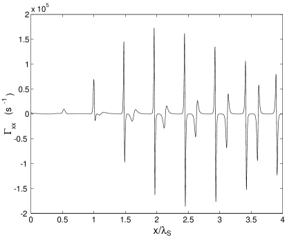
FIG. 2.: Axial friction coefficient $\Gamma_{xx}(\vec{r})$, at fixed radial distance $\rho=\rho_{\max}$ (bottom of the radial well), versus the rescaled axial coordinate $x/\lambda_{S}$, in the case (a) of opposite Stark shifts induced by the FORT mode. Parameter values are in the text.

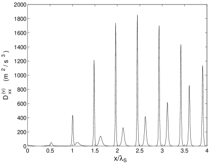
FIG. 3.: Dipole contribution to the axial velocity diffusion coefficient $D_{xx}(\vec{r})/M^{2}$, at fixed radial distance $\rho=\rho_{\max}$ (bottom of the radial well), versus the rescaled axial coordinate $x/\lambda_{S}$, in the case (a) of opposite Stark shifts induced by the FORT mode. Parameter values are in the text.

1 Simulation results

To characterize the trapping and cooling dynamics, we have carried out a quantitative study inside a central well, the one centered in $x_{5}^{e}=2.25\lambda_{S}$ and ranging from $2\lambda_{S}$ to $2.5\lambda_{S}$. In order to simulate the typical experimental condition, we have chosen proper initial conditions, considering that, in the experimental procedure, the FORT field is switched on only when the laser probe transmission exceeds a fixed threshold indicating the presence of the atom inside the cavity. The initial position has been taken axially $\lambda_{S}/8$ away from equilibrium point $x_{5}^{e}$ (then $x_{0}=2.125\lambda_{S}$), radially along the doughnut maximum $\rho_{0}=\rho_{\max}$, and uniformly distributed over the polar angle $\theta$. For what concerns the initial velocity, it is reasonable to choose a vertical velocity with components $v_{x0}=v_{y0}=0$, $v_{z0}=10$ cm/s.

In order to examine qualitatively the typical atomic motion, we report some snapshots from two simulated trajectories with slightly different initial conditions: one describes a tangential incidence of the atom along the doughnut perimeter ($x_{0}=2.125\lambda_{S}$, $y_{0}=\rho_{\max}$, $z_{0}=0$, $v_{x0}=v_{y0}=0$, $v_{z0}=10$ cm/s) (see Figs. 4-6); the other instead describes an orthogonal incidence with respect to the doughnut mode ($x_{0}=2.125\lambda_{S}$, $y_{0}=0$, $z_{0}=\rho_{\max}$, $v_{x0}=v_{y0}=0$, $v_{z0}=10$ cm/s) (see Fig. 7).

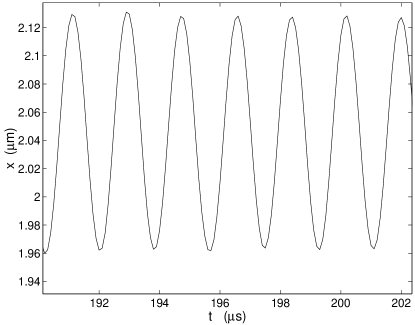
FIG. 4.: Time evolution of the axial position in the case of an initial velocity tangential with respect to the doughnut FORT mode. Parameter values are in the text.

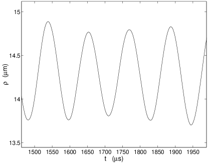
FIG. 5.: Time evolution of the radial coordinate in the case of an initial velocity tangential with respect to the doughnut FORT mode. Parameter values are in the text.

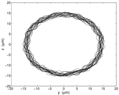
FIG. 6.: Radial trajectory in the case of an initial velocity tangential with respect to the doughnut FORT mode. Parameter values are in the text.

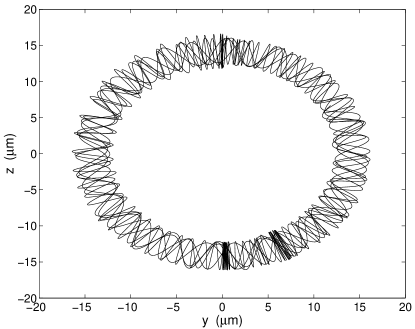
FIG. 7.: Radial trajectory in the case of an initial velocity orthogonal with respect to the doughnut FORT mode. Parameter values are in the text.

The trajectory is well confined, axially around a FORT antinode, and radially around the maximum $\rho_{\max}$: the 3D atomic motion occurs substantially on a plane orthogonal to the cavity axis, with the trajectory drawing just the shape of the doughnut mode. From Figs. 4-7 one can recognize that the atomic motion is characterized by three different time scales:

1. The fastest timescale is given by the axial oscillations, which have, for our parameter values, a time period $\sim 2\mu$s (see Fig. 4).

2. A slower timescale is associated with the radial oscillations, characterized by a time period $\sim 100$ $\mu$s (see Fig. 5); these oscillations become wider in the case of orthogonal incidence with respect to the doughnut mode, since, in this case, the atom probes more the doughnut radial elasticity (compare, in fact, Fig. 6 where the oscillation amplitude is $\sim 1$ $\mu$m with Fig. 7, where the amplitude is $\sim 4$ $\mu$m).

3. The third and slowest timescale is given by the atomic rotations around the cavity axis. For tangential incidence, the initial angular momentum is large and the rotation period is $\sim 1$ ms while, for orthogonal incidence, the atom acquires a nonzero angular momentum only because of radial diffusion, and the rotation period is larger, $\sim 10$ ms.

The final escape of the atom from the cavity is practically always along the axial direction, and this is due to the heating provided by the strong axial diffusion, which prevails with respect to the radial diffusion, determined only by the spontaneous emission.

To determine the mean trapping times, we have defined as trapping time $T$ the time spent by the atom inside a single potential well, $\lambda_{S}/2$ wide along the axial direction, and with a radius equal to $2W_{S}$. Sampling about 400 simulated trajectories, we have found the results displayed in Figs. 8 and 9.

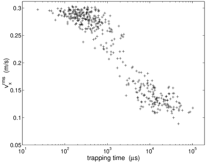
FIG. 8.: Root mean square velocity along the cavity axis $v_{x}^{rms}$ as a function of the trapping time $T$, for each simulated trajectory, in the case (a) of opposite Stark shifts.

In Fig. 8 we have displayed the root mean square velocity along the cavity axis $v_{x}^{rms}$ as a function of the trapping time $T$ for each simulated trajectory. We can see a clear separation of simulated points. In fact, about $60\%$ of atoms are not trapped at all: they correspond to the upper set of points in Fig. 8, having a velocity $v_{x}^{rms}>20$ cm/s, and for which the trapping time is below $2$ ms. These are not cooled via the cavity QED interaction, and the velocity $v_{x}^{rms}\sim 28$ cm/s is mainly a result due to the initial conditions. These uncooled atoms are those more influenced by the spatial region where the axial friction is negative (see Fig. 2), where atoms can be accelerated. The remaining $40\%$ of atoms (the points below the threshold of $20$ cm/s in Fig. 8) are trapped: their velocity $v_{x}^{rms}$ of about $14$ cm/s is a result of the cooling provided by the exchange of cavity photons. These atoms reach thermal equilibrium and have trapping times greater than $2$ ms.

Considering only the subset of trapped atoms, they have a probability $P(t)$ to be trapped for a time greater than $t$. The trapping time statistics is shown in Fig. 9, where it is also compared with a decaying fitting curve $P^{th}$ (full line in Fig. 9). The best fitting mean trapping time is $\tau=\int_{0}^{\infty}t\left(-dP^{th}/dt\right)dt=(17\pm 1)$ ms, which is comparable to the experimental value obtained using a fundamental Gaussian FORT mode in Ref. [8] and with the numerical simulations performed in [15], again for a fundamental Gaussian FORT mode. This is not surprising because, except for the fact that the atom is now trapped at a nonzero distance from the cavity axis, the physics of cooling is similar to that occurring in a lowest-order Gaussian FORT mode, and the analysis of Ref. [15] can be essentially repeated.

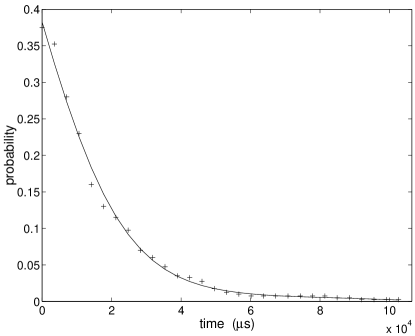
FIG. 9.: Trapping time statistics for the subset of trapped atoms in the case (a) of opposite Stark shifts. $P(t)$ is the probability for an atom to be trapped for a time greater than $t$. The full line is a fitting decay curve yielding a mean trapping time $\tau=(17\pm 1)$ ms.

B Study of case (b)

We consider the same parameter values of case (a), except that we slightly adapt the probe detuning and choose a value $\Delta_{p}=-2\pi\times 35$ MHz. As a consequence, we then set $E=22.13$ MHz, in order to keep the same empty-cavity mean photon number $N_{e}=0.01$ of case (a).

The situation is in many respects very similar to the preceding one: the atomic equilibrium positions are again situated at the FORT antinodes $x_{n}^{e}=(n-1/2)\lambda_{S}/2$, $n=1,...$ along the axial direction and at the nonzero radial distance from the cavity axis $\rho_{\max}\sim 14.1$ $\mu$m. There is still an aperiodic situation with $8$ not equivalent wells within the cavity. However, for equal atomic shifts, the FORT does not affect both friction and diffusion (it does not affect the force fluctuations, see Eqs. (20) and (21)) and therefore, for what concern friction and diffusion, an axially periodic situation is restored in this case, with a spatial period set by the cavity QED mode. The periodic friction and diffusion spatial variations are shown in Figs. 10 and 11, where the axial friction coefficient $\Gamma_{xx}(\vec{r})$ of Eqs. (20) and (22)-(24), and the dipole contribution to the axial diffusion coefficient $D_{xx}(\vec{r})$ of Eqs. (21) and (25)-(27), at fixed radial distance $\rho=\rho_{\max}$, and as a function of the axial coordinate $x$, are plotted.

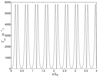
FIG. 10.: Axial friction coefficient $\Gamma_{xx}(\vec{r})$, at fixed radial distance $\rho=\rho_{\max}$ (bottom of the radial well), versus the rescaled axial coordinate $x/\lambda_{S}$, in the case (b) of equal Stark shifts induced by the FORT mode.

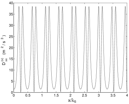
FIG. 11.: Dipole contribution to the axial velocity diffusion coefficient $D_{xx}(\vec{r})/M^{2}$, at fixed radial distance $\rho=\rho_{\max}$ (bottom of the radial well), versus the rescaled axial coordinate $x/\lambda_{S}$, in the case (b) of equal Stark shifts induced by the FORT mode.

If we compare Figs. 2 and 3 with Figs. 10 and 11 we see that in case (b) the maxima of the axial friction and diffusion coefficients are lower, but one has the advantage that now the friction coefficient is always positive, while in case (a) it may assume very large negative values, yielding heating rather than cooling. This always positive friction implies that all atoms falling in the cavity are now cooled and trapped, while in case (a), a fraction of the atoms can be heated and are not trapped.

1 Simulation results

In order to calculate the mean trapping time in case (b), we have carried out a computer simulation considering the same initial condition of case (a) (see section IV A 1). Sampling about 400 simulated trajectories, we have found the results shown in Figs. 12 and 13.

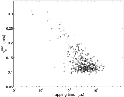
FIG. 12.: Root mean square velocity along the cavity axis $v_{x}^{rms}$ as a function of trapping time $T$, for each simulated trajectory, in the case (b) of equal Stark shifts.

In Fig. 12 we have displayed the root mean square velocity along the cavity axis $v_{x}^{rms}$ as a function of trapping time $T$ for each simulated trajectory. At variance with case (a), now all atoms are trapped, with trapping times greater than $1$ ms. This is due the fact that axial friction is always positive and atoms are cooled everywhere. In this case the probability $P(t)$ to be trapped for a time greater than $t$ (shown in Fig. 13) is computed considering all simulated points. The data are again fitted by a decaying fitting function $P^{th}(t)$ (full line in Fig. 13), yielding a mean lifetime $\tau=\int_{0}^{\infty}t\left(-dP^{th}/dt\right)dt=(44\pm 3)$ ms.

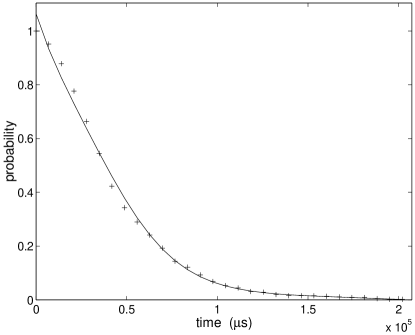
FIG. 13.: Probability $P(t)$ for an atom to be trapped for a time greater than $t$ in the case (b) of equal Stark shifts. The full line is a fitting decay curve, yielding a mean trapping time $\tau=(44\pm 3)$ ms.

This is the most relevant result of our investigation, showing that using a doughnut mode as FORT mode allows to achieve significant trapping times in the case (b), when the FORT induces equal Stark shifts on the atomic levels. In fact, we get a mean trapping time larger than that obtained, in the same situation, with a red-detuned fundamental Gaussian mode (see the numerical analysis of Ref. [15], Section IVF, where $\tau=(28\pm 2)$ ms). This shows that, in the case of equal Stark shifts, the radial confinement at a nonzero distance from the cavity axis provided by the doughnut FORT mode is preferable with respect to the radial trapping along the cavity axis provided by the TEM_0,0 FORT mode. The improvement provided by doughnut mode is useful for quantum information processing applications in cavity QED systems, because when the FORT mode induces equal shifts on the ground and excited state, the two states are trapped at the same positions within the cavity, and the internal state can be manipulated independently of its center-of-mass state. In quantum information applications, it is important to evaluate the variation of the cavity-QED coupling $\Delta g$. In our parameters’ regime it is $\Delta g\succsim 16\%$, which is worser than that for a TEM_0,0 FORT mode under the same conditions ($\Delta g\succsim 6\%$). However the problem associated with such a variation of the coupling can be circumvented if one adopts an adiabatic transfer scheme such as the one suggested in [29] for quantum information processing with hot trapped atoms. In such a case, the operation time $T_{op}$ for the adiabatic transformations must satisfy the conditions $2\mu s\sim\nu_{axial}^{-1}<T_{op}\ll\nu_{radial}^{-1}\sim 100\mu s$, where $\nu_{axial,radial}$ are the axial or radial oscillation frequencies.

An interesting alternative to the configuration studied here is to replace the TEM_0,0 cavity QED mode with the higher order LG_0,1 cavity QED mode, having the same coupling $g$ at $\rho_{\max}$. In this way we achieve a better overlap between the FORT mode and cavity QED one, which leads to a smaller variation of coupling $\Delta_{g}$, and therefore also to a better cooling configuration. In fact, repeating the simulations with the LG_0,1 cavity QED mode we have seen a slight improvement of the trapping time.

It is clear that the additional practical difficulty of using another LG mode makes the experimental realization even harder; however this should be very challenging since, extending the configuration from one LG cavity-QED mode to many degenerate LG cavity-QED modes, one has new possibilities, as following atomic motion in detail [30], or increasing the cooling effect as shown in [31].

V Discussion of the results

Let us now discuss in detail which are the main features of using red-detuned doughnut modes as FORT fields. The atom-cavity dressed picture provides an intuitive way to understand the advantages brought by the use of the doughnut mode. In the present case of very weak driving ($N_{e}=0.01$ in our case), the cooling mechanism is well described in terms of the eigenstates of the atom-cavity system (the dressed states) containing at most one excitation (see also [11, 15, 28]). The state with no excitation is the ground state $|0\rangle$, with energy $E_{0}=-\hbar S(\vec{r})$, while the first two dressed states with one excitation $|\pm\rangle$ have energies

$$E_{\pm}=\left\{\matrix{\hbar\omega_{a}\pm\hbar\sqrt{g^{2}(\vec{r})+S^{2}(\vec{r})}&{\rm case(a)}\cr\hbar\omega_{a}-\hbar S(\vec{r})\pm\hbar g(\vec{r})&{\rm case(b)}\cr}\right.,$$ (39)

so that the transition frequencies (relative to $\omega_{a}$) from the ground state $\left|0\right\rangle$ to excited states $\left|\pm\right\rangle$ have the expressions

$$\Delta_{\pm}\equiv\frac{(E_{\pm}-E_{0})}{\hbar}-\omega_{a}=\left\{\matrix{S(\vec{r})\pm\sqrt{g^{2}(\vec{r})+S^{2}(\vec{r})}&{\rm case(a)}\cr\pm g(\vec{r})&{\rm case(b)}\cr}\right..$$ (40)

The spatial variation of these transition frequencies along the axial direction (and at the radial position $\rho=\rho_{max}$) is shown in Fig. 14 for the case (a) of opposite Stark shifts, and in Fig. 15 for the case (b) of equal Stark shifts.

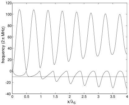
FIG. 14.: Transition frequencies $\Delta_{\pm}$ (relative to $\omega_{a}$) from the ground state $\left|0\right\rangle$ to the first excited dressed states $\left|\pm\right\rangle$ along the axial direction at fixed radial distance $\rho=\rho_{\max}$ (bottom of the radial well), in the case (a) of opposite Stark shifts. The straight line gives the probe detuning $\Delta_{p}$.

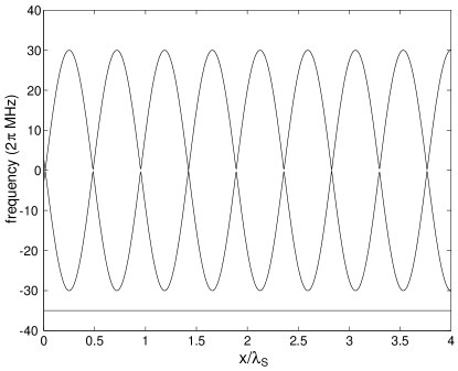
FIG. 15.: Transition frequencies $\Delta_{\pm}$ (relative to $\omega_{a}$) from the ground state $\left|0\right\rangle$ to the first excited dressed states $\left|\pm\right\rangle$ along the axial direction at fixed radial distance $\rho=\rho_{\max}$ (bottom of the radial well), in the case (b) of equal Stark shifts. The straight line gives the probe detuning $\Delta_{p}$.

The patterns of spatial variation of the transition frequency allow to understand the difference between cases (a) and (b). The cooling mechanism provided by the cavity QED interaction in the weak driving limit, can be understood in analogy with Doppler cooling. In fact, by tuning below resonance, stimulated absorption of a probe photon followed by spontaneous emission or cavity decay leads to a loss of energy. The maximum cooling rate is achieved when the excitation rate times the detuning is maximum. If the detuning turns from red to blue, cooling is replaced by heating, while if the detuning becomes more red, the atom is still cooled, but at a lower rate. In case (a) (Fig. 14), it is better to tune the probe to the lower dressed state because it has smaller spatial variations (see the straight line in Fig. 14) and it is easier to reach a compromise between having cavity regions with an optimal cooling rate (red detuning) and not too large regions with heating (blue detuning). However, as the atom moves radially from the doughnut intensity maximum at $\rho=\rho_{max}$, the situation rapidly worsens, either if the atom moves towards the center (the FORT beam decreases while the quantized field increase and the blue detuned region increases) or if tends to leave the cavity (the detuning becomes more red and the cooling rate decreases).

In case (b), one tunes again to the lowest dressed state in order to have red detuning, and therefore cooling, throughout the cavity, when the atom is at the radial equilibrium position $\rho_{max}$ (see the straight line in Fig. 15). From Eq. (40) we see that the probe detuning decreases (becomes less red) when the atom moves radially towards the center, while it becomes more red if the atom moves away radially. However, the probe detuning can be chosen so to remain always red: in this way the atom is cooled everywhere, and is never accelerated. For this reason the doughnut FORT mode provides longer trapping times in case (b) of equal Stark shifts rather than in case (a) of opposite shifts. What is more important is that, in case (b), the doughnut FORT mode provides longer trapping times than a fundamental Gaussian FORT mode (see [15], Section IVF). In fact, in the latter case, the probe detuning would be tuned so to have optimal cooling on the cavity axis, where the atoms will be now trapped. However, because of radial diffusion (due to spontaneous emission) which also leads to an increasing angular momentum and the consequent rising of a centrifugal potential, the atom tends to move radially away from the cavity axis, so that the optimal cooling condition is rapidly lost. In fact, for increasing $\rho$, the axial pattern of Fig. 15 rapidly vanishes, the driving probe becomes too far-off resonance and the cooling efficiency is lost.

The advantage of the doughnut FORT with respect to the TEM_0,0 FORT is that it imposes a much sharper radial well around the equilibrium position corresponding to the optimum cooling condition. The atom is less free to move radially, and moreover is subject to a smaller centrifugal force because it is trapped by the doughnut at a larger radial distance from the cavity axis. In other words, the radial potential well provided by the doughnut FORT mode is more suitable to counteract the radial departure of the atom and so to preserve the optimal cooling condition.

The importance of a strong radial confinement to optimize cooling and trapping in the case of equal Stark shifts can be illustrated also checking that when the width of the radial well is decreased, the trapping time increases. To this purpose, we have carried out a simulation where a higher order Laguerre-Gauss FORT mode, LG_0,12, is used instead of the LG_0,1 FORT mode, keeping the other conditions unchanged. To be more specific, we have considered the same experimental parameters of the case with the LG_0,1 FORT mode in case (b), in such a way that the LG_0,12 mode gives the same Stark shift $S_{\max}=2\pi\times 50$ MHz at the same radial distance $\rho_{\max}\sim 14.1$ $\mu m$. This means adapting both the incident FORT power and the doughnut mode waist, so that the only difference with the case studied in the preceding Section is the smaller width of the radial well (see Fig. 16, where the radial profile of the Stark shift induced by the LG_0,12 FORT mode is compared with that of the LG_0,1 mode). The chosen parameters are the same as above except that now the spatial dependence of the Stark shift (equal for both ground and excited state) is

$$S(\rho,x)=S_{0}\rho^{24}\sin^{2}(k_{S}x)\exp\left\{\frac{-2\rho^{2}}{W_{S}^{2}}\right\},$$ (41)

with $W_{S}=20/\sqrt{12}\sim 5.77$ $\mu$m and $S_{0}\sim 1.2\times 10^{-20}$ MHz$/\mu$m²⁴.

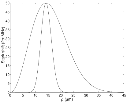
FIG. 16.: Stark shifts $S_{0,1}$ and $S_{0,12}$ (narrower curve) as a function of the radial coordinate $\rho$, at the axial antinode. Parameter values are in the text.

Considering again the initial conditions specified in Section IV A 1 and sampling about 400 simulated trajectories, we have found the results shown in Figs. 17 and 18.

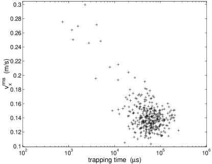
FIG. 17.: Root mean square velocity along the cavity axis $v_{x}^{rms}$ as a function of trapping time $T$, for each simulated trajectory in the case (b) and with the higher order FORT mode LG_0,12.

In Fig. 17 we have displayed the root mean square velocity along the cavity axis $v_{x}^{rms}$ as a function of trapping time $T$ for each simulated trajectory. All atoms are again trapped, with trapping times greater than $1$ ms. The probability $P(t)$ to be trapped for a time greater than $t$ (shown in Fig. 18) is computed considering all simulated points. The data are again fitted by a decaying fitting function $P^{th}(t)$ (full line in Fig. 18), yielding a mean lifetime $\tau=\int_{0}^{\infty}t\left(-dP^{th}/dt\right)dt=(64\pm 5)$ ms.

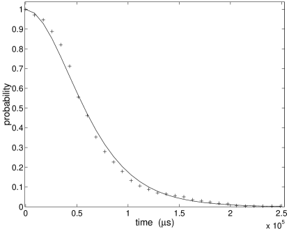
FIG. 18.: Probability $P(t)$ for an atom to be trapped for a time greater than $t$ in the case (b) and with the higher order FORT mode LG_0,12. The full line is a fitting decay curve yielding a mean trapping time $\tau=(64\pm 5)$ ms.

This significant improvement in the mean trapping time, provided by the LG_0,12 FORT mode with respect to the LG_0,1 one, is due to the strongest radial confinement achieved (see Fig. 16). The atom stays closer to the radial potential minimum where cooling conditions are optimized and the probability to leave the cavity decreases. This is a further argument showing that the main advantage of using a doughnut FORT mode instead of a TEM_0,0 FORT mode for atom trapping in the case of equal Stark shifts is just the stronger radial confinement which makes easier to optimize the cooling conditions. The more the atom is radially confined, the longer is trapped.

Here we have decreased the width of the radial well by choosing a higher order doughnut mode and by simultaneously adjusting its waist, so to have an unchanged radial equilibrium position $\rho_{max}$. This solution may be practically difficult to implement because one would need different cavity mirrors for this high-order doughnut FORT mode. Anyway, even though the implementation of the trapping scheme with a higher-order doughnut mode is difficult, the latter numerical results clearly show the importance of the radial confinement, and the direction one has to follow in order to increase the trapping time of neutral atoms in cavities in the case of equal Stark shifts induced by the FORT mode.

A possible solution to overcome the practical difficulties of a LG_0,12 experimental set-up can be the following one, provided that one has enough power and stability for the laser driving the FORT mode. The same radial potential around $\rho_{\max}$ as that created by the LG_0,12 FORT mode can be achieved using a very intense LG_0,1 FORT mode. One can take $S_{0}=4\pi e$ MHz/$\mu$m², leading to $S_{max}=2\pi\times 400$ MHz, and leave all the other parameters unchanged (see IV.B for the parameters of the LG_0,1 FORT mode in case (b)). In this new configuration, both the radial and the axial wells are 8 times deeper, and therefore, together with the desired strong radial confinement (substantially the same as that of LG_0,12 FORT mode), we have a strong axial confinement. Both these facts lead to a considerable increase of trapping time, up to $2$ seconds (a result of the same order as the one recently reported in [21]), as demonstrated by the numerical simulation of some trajectories which we show in the following table:

trapping time $$\tau$$       eq. temp.         type of escape

157 29.4      axial

432 20.2      axial

556 16.1      axial

684 13.7       radial

1107 10.5       radial

1108 11.4       radial

1177 10.7       radial

2141 10.4       radial

(42)

According to table (42), the atom is so strongly confined axially that in some cases (those with the longer trapping times), it leaves the cavity radially, due to the effect of spontaneous emission. In these cases, an additional radial cooling mechanism would be helpful as, for instance, that achieved via an additional transverse free-space cooling (see [21]) or via an active feedback on radial motion [14].

VI Conclusions

We have investigated trapping of single atoms in high finesse optical cavities using both a quasi-resonant cavity QED field and an intense classical FORT mode. In particular we have considered the case of doughnut FORT modes, and we have compared them to the most common case of a fundamental Gaussian FORT mode (see for example the experiment of Ref. [8]). Performing full 3-D numerical simulations of the quasi-classical center-of-mass motion of the atom, we have shown that a doughnut FORT mode is more suitable than a fundamental Gaussian FORT mode to trap the atom, in the case when the FORT mode shifts both the excited and the ground state down. This happens when the FORT mode is red-detuned in such a way that the excited state is relatively closer to resonance with a higher-lying excited state than with the ground state. This case, even though more difficult to realize than the standard two-level case where the two Stark shifts are opposite, is of particular interest for quantum information applications of cavity-QED systems, where it is important to trap the atom at a given position, independently of its internal state, so that the quantum manipulation of the internal state can be easily performed. The advantage of using a doughnut FORT mode instead of a TEM_0,0 one is due to the stronger radial confinement, achieved at a nonzero distance from the cavity axis. In this way the FORT mode is more suitable to counteract the unavoidable radial departure caused by the centrifugal potential and by diffusion, by keeping the atom close to its equilibrium position where the cooling provided by the quantized cavity mode is optimal.

VII Acknowledgments

This work has been partially supported by the European Union through the IHP program “QUEST”.

REFERENCES

- [1] Cavity Quantum Electrodynamics, Advances in Atomic, Molecular and Optical Physics, Supplement 2, edited by P. Berman (Academic, New York, 1994)
- [2] Q. A. Turchette, C. J. Hood, W. Lange, H. Mabuchi and H. J. Kimble, Phys. Rev. Lett. 75, 4710 (1995).
- [3] B. T. H. Varcoe, S. Brattke, M. Weidinger, H. Walther, Nature 403, 743 (2000).
- [4] G. Nogues, A. Rauschenbeutel, S. Osnaghi, M. Brune, J. M. Raimond, S. Haroche, Nature 400, 239 (1999).
- [5] T. Pellizzari it et al., Phys. Rev. Lett. 75, 3788 (1995); J. I. Cirac, P. Zoller, H. J. Kimble, and H. Mabuchi, Phys. Rev. Lett. 78, 3221 (1997); S. J. Van Enk, J. I. Cirac, and P. Zoller , Phys. Rev. Lett. 78, 4293 (1997); Science 279, 205 (1998).
- [6] C. J. Hood, T. W. Lynn, A. C. Doherty, A. S. Parkins, and H. J. Kimble, Science 287, 1447 (2000).
- [7] P. V. H. Pinkse, T. Fischer, P. Maunz, and G. Rempe, Nature 404, 365 (2000).
- [8] J. Ye, D. W. Vernooy, and H. J. Kimble, Phys. Rev. Lett. 83, 4987 (1999).
- [9] H. Mabuchi et al. Opt. Lett. 21, 1393 (1996); C. J. Hood et al. Phys. Rev. Lett. 80, 4157 (1998); P. Münstermann, T. Fischer, P. Maunz, P. W. Pinkse, and G. Rempe, ibid. 82, 3791 (1999).
- [10] T. W. Mossberg, M. Lewenstein, and D. J. Gauthier, Phys. Rev. Lett. 67, 1723 1991; M. Lewenstein and L. Roso, Phys. Rev. A 47, 3385 (1993); J. I. Cirac, M. Lewenstein, and P. Zoller, Phys. Rev. A 51, 1650 (1995); A. C. Doherty, A. S. Parkins, S. M. Tan, and D. F. Walls, ibid. 56, 833 (1997).
- [11] P. Horak, G. Hechenblaikner, K. M. Gheri, H. Stecher, and H. Ritsch, Phys. Rev. Lett. 79, 4974 (1997); G. Hechenblaikner, M. Gangl, P. Horak, and H. Ritsch, Phys. Rev. A 58, 3030 (1998); P. Domokos, P. Horak, and H. Ritsch, J. Phys. B: At. Mol. Opt. Phys. 34. 187 (2001).
- [12] V. Vuletić and S. Chu, Phys. Rev. Lett. 84, 3787 (1999); V. Vuletić, H. W. Chan and A. T. Black, Phys. Rev. A 64, 033405 (2001).
- [13] A. C. Doherty, T. W. Lynn, C. J. Hood, and H. J. Kimble, Phys. Rev. A 63, 013401 (2001).
- [14] T. Fischer, P. Maunz, P. W. H. Pinkse, T. Puppe, and G. Rempe, Phys. Rev. Lett. 88, 163002 (2002).
- [15] S. J. van Enk, J. McKeever, H. J. Kimble, and J. Ye, Phys. Rev. A 64, 013407 (2001).
- [16] J. Dalibard and C. Cohen-Tannoudji, J. Phys. B: At. Mol. Opt. Phys. 18 1661 (1985).
- [17] A. Siegman. Lasers. University Sciences, Mill Valley (1986)
- [18] J. D. Miller, R. A. Cline, and D. J. Heinzen, Phys. Rev. A 47, R4567 (1993).
- [19] This is possible for Cs atoms in correspondence with FORT wavelengths from 920 upward, as shown in [20] where, in particular, the special wavelength causes an identical shift for the levels. Recently also the ’magic’ wavelength has been used in [21]
- [20] H. J. Kimble, C. J. Hood, T. W. Lynn, H. Mabuchi, D. W. Vernooy, and J. Ye, Laser Spectroscopy XIV, Eds. R. Blatt, J. Eschner, D. Leibfried, and F. Schmidt-Kaler, World Scientific (Singapore, 1999).
- [21] J. McKeever, J. R. Buck, A. D. Boozer, A. Kuzmich, H. C. Nagerl, D. M. Stamper-Kurn, and H. J. Kimble, quant-ph/0211013 v1 (2002).
- [22] T. A. Savard , K. M. O’Hara, and J. E. Thomas, Phys. Rev. A 56, R1095 (1997).
- [23] C. W. Gardiner, J. Ye, H. C. Nagerl, and H. J. Kimble, Phys. Rev. A 61, 045801 (2000).
- [24] J. Javanainen and S. Stenholm, Appl. Phys. 21, 35 (1980).
- [25] H. Risken, The Fokker-Planck Equation, 2nd Edition (Springer, 1989).
- [26] C. W. Gardiner, Handbook of Stochastic Methods for Physics, Chemistry and the Natural Sciences, 2nd Edition (Springer-Verlag, Berlin, 1985).
- [27] S. M. Tan, J. Opt. B 1, 424 (1999). S. M. Tan’s Quantum Optics Toolbox at www.phy.auckland.ac.nz/Staff/smt/qotoolbox/download.html.
- [28] D. W. Vernooy and H. J. Kimble, Phys. Rev. A 56, 4287 (1997).
- [29] L.-M. Duan, A. Kuzmich, and H. J. Kimble, quant-ph/0208051 (2002).
- [30] P. Horak, H. Ritsch, T. Fischer, P. Maunz, T. Puppe, P. W. H. Pinkse, and G. Rempe, Phys. Rev. Lett. 88, 043601 (2002).
- [31] P. Horak and H. Ritsch, Phys. Rev. A 64, 033422 (2001).