Quantization, group contraction and zero point energy

Abstract

We study algebraic structures underlying ’t Hooft’s construction relating classical systems with the quantum harmonic oscillator. The role of group contraction is discussed. We propose the use of $SU(1,1)$ for two reasons: because of the isomorphism between its representation Hilbert space and that of the harmonic oscillator and because zero point energy is implied by the representation structure. Finally, we also comment on the relation between dissipation and quantization.

]

I Introduction

Recently, the “close relationship between quantum harmonic oscillator (q.h.o.) and the classical particle moving along a circle” has been discussed [1] in the frame of ’t Hooft conjecture [2] according to which the dissipation of information which would occur at a Planck scale in a regime of completely deterministic dynamics would play a role in the quantum mechanical nature of our world. In particular, ’t Hooft has shown that in a certain class of classical, deterministic systems, the constraints imposed in order to provide a bounded from below Hamiltonian, introduce information loss and lead to “an apparent quantization of the orbits which resemble the quantum structure seen in the real world”.

Consistently with this scenario, it has been explicitly shown [3] that the dissipation term in the Hamiltonian for a couple of classical damped-amplified oscillators [4, 5, 6] is actually responsible for the zero point energy in the quantum spectrum of the 1D linear harmonic oscillator obtained after reduction. Such a dissipative term manifests itself as a geometric phase and thus the appearance of the zero point energy in the spectrum of q.h.o can be related with non-trivial topological features of an underlying dissipative dynamics.

The purpose of this paper is to further analyze the relationship discussed in [1] between the q.h.o. and the classical particle system, with special reference to the algebraic aspects of such a correspondence.

’t Hooft’s analysis, based on the $SU(2)$ structure, uses finite dimensional Hilbert space techniques for the description of the deterministic system under consideration. Then, in the continuum limit, the Hilbert space becomes infinite dimensional, as it should be to represent the q.h.o.. In our approach, we use the $SU(1,1)$ structure where the Hilbert space is infinite dimensional from the very beginning.

We show that the relation foreseen by ’t Hooft between classical and quantum systems, involves the group contraction [7] of both $SU(2)$ and $SU(1,1)$ to the common limit $h(1)$. The group contraction completely clarifies the limit to the continuum which, according to ’t Hooft, leads to the quantum systems.

We then study the $D^{+}_{k}$ representation of $SU(1,1)$ and find that it naturally provides the non-vanishing zero point energy term. Due to the remarkable fact that $h(1)$ and the $D^{+}_{k}$ representations share the same Hilbert space, we are able to find a one-to-one mapping of the deterministic system represented by the $D^{+}_{1/2}$ algebra and the q.h.o. algebra $h(1)$. Such a mapping is realized without recourse to group contraction, instead it is a non-linear realization similar to the Holstein-Primakoff construction for $SU(2)$ [8].

Our treatment sheds some light on the relationship between the dissipative character of the system Hamiltonian (formulated in the two-mode $SU(1,1)$ representation) and the zero point energy of the q.h.o., in accord with the conclusions presented in Ref.[3].

II ’t Hooft’s scenario

As far as possible we will closely follow the presentation and the notation of Ref. [1]. We start by considering the discrete translation group in time $T_{1}$. ’t Hooft considers the deterministic system consisting of a set of $N$ states, $\{(\nu)\}\equiv\{(0),(1),...(N-1)\}$, on a circle, which may be represented as vectors:

$$(0)=\left(\begin{array}[]{c}0\\ 0\\ \vdots\\ 1\end{array}\right);\,(1)=\left(\begin{array}[]{c}1\\ 0\\ \vdots\\ 0\end{array}\right);\dots;(N-1)=\left(\begin{array}[]{c}0\\ \vdots\\ 1\\ 0\end{array}\right),$$ (13)

and $(0)\equiv(N)$. The time evolution takes place in discrete time steps of equal size, $\Delta t=\tau$

$$t\to t+\tau\quad:\quad(\nu)\to(\nu+1~{}~{}{\rm mod}~{}N)$$ (14)

and thus is a finite dimensional representation $D_{N}(T_{1})$ of the above mentioned group. On the basis spanned by the states $(\nu)$, the evolution operator is introduced as [1] (we use $\hbar=1$):

$$U(\Delta t=\tau)\,=\,e^{-iH\tau}\,=\,e^{-i\frac{\pi}{N}}\left(\begin{array}[]{ccccc}0&&&&1\\ 1&0&&&\\ &1&0&&\\ &&\ddots&\ddots&\\ &&&1&0\end{array}\right)$$ (20)

This matrix satisfies the condition $U^{N}=1{\rm I}$ and it can be diagonalized by a suitable transformation. The phase factor in Eq.(20) is introduced by hand. It gives the $1/2$ term contribution to the energy spectrum of the eigenstates of $H$ denoted by $|n\rangle$, $n=0,1,...N-1$:

$$\frac{H}{\omega}~{}~{}|n\rangle~{}~{}=~{}~{}(n+\frac{1}{2})~{}|n\rangle~{},~{}~{}~{}~{}\omega\equiv\frac{2\pi}{N\tau}.$$ (21)

The Hamiltonian $H$ in Eq.(21) seems to have the same spectrum of the Hamiltonian of the harmonic oscillator. However it is not so, since its eigenvalues have an upper bound implied by the finite $N$ value (we have assumed a finite number of states). Only in the continuum limit ($\tau\to 0$ and $l\to\infty$ with $\omega$ fixed, see below) one will get a true correspondence with the harmonic oscillator.

The system of Eq.(13) is plotted in Fig. 1 for $N=7$. An underlying continuous dynamics is introduced, where $x(t)=\cos(\alpha t)\cos(\beta t)$ and $y(t)=-\cos(\alpha t)\sin(\beta t)$. At the times $t_{j}=j\pi/\alpha$, with $j$ integer, the trajectory touches the external circle, i.e. $R^{2}(t_{j})=x^{2}(t_{j})+y^{2}(t_{j})=1$, and thus $\pi/\alpha$ is the frequency of the discrete (’t Hooft) system. At time $t_{j}$, the angle of $R(t_{j})$ with the positive x axis is given by: $\theta_{j}=j\pi-\beta t_{j}=j(1-\beta/\alpha)\pi$. When $\beta/\alpha$ is a rational number, of the form $q=M/N$, the system returns to the origin (modulo $2\pi$) after $N$ steps. To ensure that the $N$ steps cover only one circle, we have to impose $\alpha(t_{j})=j\,2\pi/N$, which gives the condition $M=N-2$. Thus, in order to reproduce ’t Hooft’s system for $N=7$, as in Fig. 1, we choose $q=5/7$. For $N=8$, we have $q=3/4$ and so on.

      

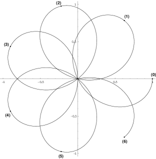
FIG. 1.: ’t Hooft’s deterministic system for $N=7$.

 

The system of Eq.(13) can be described in terms of an $SU(2)$ algebra if we set

$$N\equiv 2l+1~{},~{}~{}~{}n\equiv m+l~{},~{}~{}~{}~{}m\equiv-l,...,l~{},$$ (22)

so that, by using the more familiar notation $|l,m\rangle$ for the states $|n\rangle$ in Eq.(21) and introducing the operators $L_{+}$ and $L_{-}$ and $L_{3}$, we can write the set of equations

$$\frac{H}{\omega}~{}|l,m\rangle = (n+\frac{1}{2})~{}|l,m\rangle\,.$$ (23)

$$L_{3}~{}|l,m\rangle = m~{}|l,m\rangle\,,$$ (24)

$$L_{+}~{}|l,m\rangle = \sqrt{(2l-n)(n+1)}~{}|l,m+1\rangle\,,$$ (25)

$$L_{-}~{}|l,m\rangle = \sqrt{(2l-n+1)n}~{}|l,m-1\rangle\,.$$ (26)

with the $su(2)$ algebra being satisfied $(L_{\pm}\equiv L_{1}\pm iL_{2})$:

$$[L_{i},L_{j}\,]=i\epsilon_{ijk}L_{k}~{},~{}~{}i,j,k=1,2,3.$$ (27)

’t Hooft then introduces the analogues of position and momentum operators:

$${\hat{x}}\equiv\alpha L_{x},\quad{\hat{p}}\equiv\beta L_{y},~{}~{}\alpha\equiv\sqrt{\frac{\tau}{\pi}},~{}~{}\beta\equiv\frac{-2}{2l+1}\sqrt{\frac{\pi}{\tau}}\,,$$ (28)

satisfying the “deformed” commutation relations

$$[{\hat{x}},{\hat{p}}\,]\,=\,\alpha\beta iL_{z}\,=\,i\left(1-\frac{\tau}{\pi}H\right)\,.$$ (29)

The Hamiltonian is then rewritten as

$$H\,=\,\frac{1}{2}\omega^{2}{\hat{x}}^{2}\,+\,\frac{1}{2}{\hat{p}}^{2}\,+\,\frac{\tau}{2\pi}\left(\frac{\omega^{2}}{4}+H^{2}\right)\,.$$ (30)

The continuum limit is obtained by letting $l\to\infty$ and $\tau\to 0$ with $\omega$ fixed for those states for which the energy stays limited. In such a limit the Hamitonian goes to the one of the harmonic oscillator, the ${\hat{x}}$ and ${\hat{p}}$ commutator goes to the canonical one and the Weyl-Heisenberg algebra $h(1)$ is obtained. In that limit the original state space (finite $N$) changes becoming infinite dimensional. We remark that for non-zero $\tau$ Eq.(29) reminds the case of dissipative systems where the commutation relations are time-dependent thus making meaningless the canonical quantization procedure [4].

We now show that the above limiting procedure is nothing but a group contraction. One may indeed define  $a^{\dagger}\equiv L_{+}/\sqrt{2l}$,  $a\equiv L_{-}/\sqrt{2l}$  and, for simplicity, restore the $|n\rangle$ notation ($n=m+l$) for the states:

$$\frac{H}{\omega}~{}|n\rangle = (n+\frac{1}{2})~{}|n\rangle$$ (31)

$$a^{\dagger}~{}|n\rangle = \sqrt{\frac{(2l-n)}{2l}}\sqrt{n+1}~{}|n+1\rangle\,,$$ (32)

$$a~{}|n\rangle = \sqrt{\frac{2l-n+1}{2l}}\sqrt{n}~{}|n-1\rangle\,.$$ (33)

The continuum limit is then the contraction $l\to\infty$ (fixed $\omega$):

$$\frac{H}{\omega}~{}|n\rangle = (n+\frac{1}{2})~{}|n\rangle\,.$$ (34)

$$a^{\dagger}~{}|n\rangle = \sqrt{n+1}~{}|n+1\rangle\,,$$ (35)

$$a~{}|n\rangle = \sqrt{n}~{}|n-1\rangle\,,$$ (36)

and, by inspection,

$$[a,a^{\dagger}]~{}|n\rangle = ~{}|n\rangle$$ (37)

$$\{a^{\dagger},a\}~{}|n\rangle = 2(n+1/2)~{}|n\rangle.$$ (38)

We thus have $[a,a^{\dagger}]=1$ and $H/\omega=\frac{1}{2}\{a^{\dagger},a\}$ on the representation $\{|n\rangle\}$. With the usual definition of $a$ and $a^{\dagger}$, one obtains the canonical commutation relations $[{\hat{x}},{\hat{p}}]=i$ and the standard Hamiltonian of the harmonic oscillator.

We note that the underlying Hilbert space, originally finite dimensional, becomes infinite dimensional, under the contraction limit. Then we are led to consider an alternative model where the Hilbert space is not modified in the continuum limit.

III The $SU(1,1)$ systems

The above model is not the only example one may find of a deterministic system which reduces to the quantum harmonic oscillator. For instance, we may consider deterministic systems based on the non compact group $SU(1,1)$. An example is the system depicted in Fig. 2: It consists of two subsystems, each of them made of a particle moving along a circle in discrete equidistant jumps. Both particles and circle radii might be different, the only common thing is that both particles are synchronized in their jumps. We further assume that for both particles the ratio (circumference)/(length of the elementary jump) is an irrational number (generally different) so that particles never come back into the original position after a finite number of jumps. We shall label the corresponding states (positions) as $(n)_{A}$ and $(n)_{B}$ respectively. The plot in Fig. 2 is obtained by using the same continuous dynamics as for Fig. 1 with $\beta/\alpha=5/3+\pi/40$.

The synchronized time evolution is by discrete and identical time steps $\triangle t=\tau$ as follows:

$$t\rightarrow t+\tau\,\,\,\,; (1)_{A}\rightarrow(2)_{A}\rightarrow(3)_{A}\rightarrow(4)_{A}\ldots\,,$$

$$(1)_{B}\rightarrow(2)_{B}\rightarrow(3)_{B}\rightarrow(4)_{B}\ldots\,.$$

      

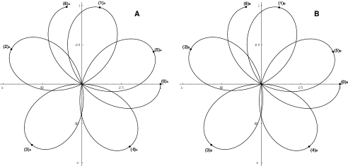
FIG. 2.: A deterministic system based on $SU(1,1)$.

 

This evolution is, of course, completely deterministic. A practical realization of one of such particle subsystem is in fact provided by a charged particle in the cylindrical magnetron, which is a device with a radial, cylindrically symmetric electric field that has in addition a perpendicular uniform magnetic field. Then the particle trajectory is basically a cycloid which is wrapped around the center of the magnetron. The actual parameters of the cycloid are specified by the Larmor frequency $\omega_{L}=qB/2m$. To implement the discrete time evolution we confine ourself only to an observation of the largest radius positions of the particle. So we disregard any information concerning the actual underlying trajectory. If the the Larmor frequency and orbital frequency are incommensurable then the particle proceeds via discrete time evolution with $\tau=2\pi/\omega_{L}$ and returns into its initial position only after infinitely many revolutions.

The actual states (positions) can be represented by vectors similar in structure to the ones in Eq.(13) with the important difference that in the present case the number $N$ of their components is infinite. The one–time–step evolution operator acts on $(n)_{A}\otimes(m)_{B}$ and in the representation space of the states it reads

$$U(\tau)\, \equiv \,e^{-iH\tau}\,=\,e^{-iH_{A}\tau}\otimes e^{-iH_{B}\tau}$$ (39)

$$= \left(\begin{array}[]{cccc}0&0&\ldots&1\\ 1&0&\ldots&0\\ 0&1&\ldots&0\\ &\ddots&\ddots\end{array}\right)_{A}\otimes\left(\begin{array}[]{cccc}0&0&\ldots&1\\ 1&0&\ldots&0\\ 0&1&\ldots&0\\ &\ddots&\ddots\end{array}\right)_{B}\,.$$ (48)

As customary one works with finite dimensional matrices and at the end of the computations the infinite dimensional limit is considered.

It is worth to mentionthat our system consisting of two particles “jumping” along two circles can, in fact, be realized with only a single particle “jumping” on a 2D torus. Assuming that $\varphi_{1}$ and $\varphi_{2}$ are angular coordinates (longitude and latitude) on the 2D torus we prescribe the one–time–step evolution as

$$t\rightarrow t+\tau\,;\;\;\;\; \varphi_{1}\rightarrow\varphi_{1}+\alpha_{1}\tau\,,$$ (50)

$$\varphi_{2}\rightarrow\varphi_{2}+\alpha_{2}\tau\,.$$

Note that while the discrete time evolution on latitude circle stays on the latitude circle, the discrete time evolution along longitude does not preserve the longitude circle but deforms it into “winding line”. This is not in contradiction with the previous two–circle model.In reality, the (common) key point is that after infinite (and only infinite) time the system returns into the original position. In fact, in the torus system if $\alpha_{1}/\alpha_{2}$ is irrational then the positions (states) never return back into the original configuration at any finite time but instead they fill up all the torus surface (they are dense in the torus [9]). Inasmuch the states (positions) are dense along both “circles” separately and return into the initial position after infinitely long time. We will not consider in this paper further details of these systems since we are here interested mainly in their algebraic description and in the matching with the quantum oscillator in the continuous limit.

The advantage with respect to the previous $SU(2)$ case is now that the non-compactness of $SU(1,1)$ guarantees that only the matrix elements of the rising and lowering operators are modified in the contraction procedure. Since the $SU(1,1)$ group is well known (see e.g. [10]), we only recall that it is locally isomorphic to the (proper) Lorentz group in two spatial dimensions $SO(2,1)$ and it differs from $SU(2)$ only in a sign in the commutation relation: $[L_{+},L_{-}]=-2L_{3}$. $SU(1,1)$ representations are well known, in particular the discrete series $D^{+}_{k}$ is

$$L_{3}|n\rangle = (n+k)|n\rangle\,,$$ (51)

$$L_{+}|n\rangle = \sqrt{(n+2k)(n+1)}|n+1\rangle\,,$$ (52)

$$L_{-}|n\rangle = \sqrt{(n+2k-1)n}|n-1\rangle\,,$$ (53)

where, like in $h(1)$, $n$ is any integer greater or equal to zero and the highest weight $k$ is a non-zero positive integer of half-integer number.

In order to study the connection with the quantum harmonic oscillator, we set

$$H/\omega=L_{3}-k+1/2~{}.$$ (54)

$$a^{\dagger}=L_{+}/\sqrt{2k}~{},~{}~{}~{}~{}a=L_{-}/\sqrt{2k}.$$ (55)

The $SU(1,1)$ contraction $k\to\infty$ again recovers the quantum oscillator Eqs.(36), (38), i.e. the $h(1)$ algebra. From (53), as announced, we see that the contraction $k\to\infty$ does not modify $L_{3}$ and its spectrum but only the matrix elements of $L_{\pm}$. The relevant point is that, while in the $SU(2)$ case the Hilbert space gets modified in the contraction limit, in the present $SU(1,1)$ case the Hilbert space is not modified in such a limit: a mathematically well founded perturbation theory can be now formulated (starting from Eqs.(53), with perturbation parameter $\propto{1/k}$) in order to recover the wanted Eqs.(36) in the contraction limit.

IV The zero point energy

We now concentrate on the phase factor in Eq.(20), which fixes the zero point energy in the oscillator spectrum. It is well known that the zero point energy is the true signature of quantization and is a direct consequence of the non-zero commutator of $\hat{x}$ and $\hat{p}$. Thus this is a crucial point in the present analysis.

The $SU(2)$ model considered in Section II says nothing about the inclusion of the phase factor.

On the other hand, it is remarkable that the $SU(1,1)$ setting, with $H=\omega L_{3}$, always implies a non-vanishing phase, since $k>0$. In particular, the fundamental representation has $k=1/2$ and thus

$$L_{3}|n\rangle = (n+1/2)|n\rangle\,,$$ (56)

$$L_{+}|n\rangle = (n+1)|n+1\rangle\,,$$ (57)

$$L_{-}|n\rangle = n|n-1\rangle\,.$$ (58)

We note that the rising and lowering operator matrix elements do not carry the square roots, as on the contrary happens for $h(1)$ (cf. e.g. Eqs.(36)).

Then we introduce the following mapping in the universal enveloping algebra of $su(1,1)$:

$$a=\frac{1}{\sqrt{L_{3}+1/2}}\,L_{-}\quad;\quad a^{\dagger}=L_{+}\,\frac{1}{\sqrt{L_{3}+1/2}}$$ (59)

which gives us the wanted $h(1)$ structure of Eq.(36), with $H=\omega L_{3}$. Note that now no limit (contraction) is necessary, i.e. we find a one-to-one (non-linear) mapping between the deterministic $SU(1,1)$ system and the quantum harmonic oscillator. The reader may recognize the mapping Eq.(59) as the non-compact analog [11] of the well-known Holstein-Primakoff representation for $SU(2)$ spin systems [8, 12].

We remark that the $1/2$ term in the $L_{3}$ eigenvalues now is implied by the used representation. Moreover, after a period $T=2\pi/\omega$, the evolution of the state presents a phase $\pi$ that it is not of dynamical origin: $e^{-iHT}\neq 1$, it is a geometric-like phase (remarkably, related to the isomorphism between $SO(2,1)$ and $SU(1,1)/Z_{2}$  ($e^{i2\times 2\pi L_{3}}=1$)). Thus the zero point energy is strictly related to this geometric-like phase (which confirms the result of Ref. [3]).

V The dissipation connection

Eqs.(53) and (58) suggest to us one more scenario where we may recover the already known connection [2, 3] between dissipation and quantization. Indeed, by introducing the Schwinger-like two mode $SU(1,1)$ realization in terms of $h(1)\otimes h(1)$, the square roots in the eigenvalues of $L_{+}$ and $L_{-}$ in Eq.(58) may also be recovered. We set:

$$L_{+}\equiv{A^{\dagger}}B^{\dagger}\quad,\quad L_{-}\equiv AB\equiv{L_{+}}^{\dagger},$$ (60)

$$L_{3}\equiv{\frac{1}{2}}(A^{\dagger}A+B^{\dagger}B+1),$$ (61)

with $[A,A^{\dagger}]=[B,B^{\dagger}]=1$ and all other commutators equal to zero. The Casimir operator is ${\cal C}^{2}=1/4+L_{3}^{2}-1/2(L_{+}L_{-}+L_{-}L_{+})=1/4(A^{\dagger}A-B^{\dagger}B)^{2}$.

We now denote by $\{|n_{A},n_{B}\rangle\}$ the set of simultaneous eigenvectors of the $A^{\dagger}A$ and $B^{\dagger}B$ operators with $n_{A}$, $n_{B}$ non-negative integers. We may then express the states $|n\rangle$ in terms of the basis $|j,m\rangle$, with $j$ integer or half-integer and $m\geq|j|$, and

$${\cal C}|j,m\rangle = j|j,m\rangle,~{}~{}~{}~{}~{}~{}~{}j=1/2(n_{A}-n_{B})~{},$$ (62)

$$L_{3}|j,m\rangle = (m+1/2)|j,m\rangle,~{}~{}~{}m=1/2(n_{A}+n_{B})~{},$$ (63)

where $n=m-|j|$ and $k=|j|+1/2$ (cf. Eq.(53)). Clearly, for $j=0$, i.e. $n=n_{A}=n_{B}$, we have the fundamental representation (58) and $L_{-}|n\rangle=AB|n\rangle={\sqrt{n}}{\sqrt{n}}|n\rangle=n|n\rangle$ (and similarly for $L_{+}$). This accounts for the absence of square roots in Eqs.(58).

In order to clarify the underlying physics, it is convenient to change basis: $|\phi_{j,m}\rangle\equiv e^{{\frac{\pi}{2}}L_{1}}|j,m\rangle$. By exploiting the relation [4]

$$i~{}e^{{\frac{\pi}{2}}L_{1}}~{}L_{3}~{}e^{-{\frac{\pi}{2}}L_{1}}~{}~{}=~{}~{}L_{2}~{},$$ (64)

we have

$$L_{2}~{}|\phi_{j,m}\rangle~{}=~{}i~{}(m+1/2)~{}|\phi_{j,m}\rangle~{}.$$ (65)

Here it is necessary to remark that one should be careful in handling the relation (64) and the states $|\phi_{j,m}\rangle$. In fact Eq.(64) is a non-unitary transformation in $SU(1,1)$ and the states $|\phi_{j,m}\rangle$ do not provide a unitary irreducible representation (UIR). They are indeed not normalizable states [13, 14] (in any UIR of $SU(1,1)$, $L_{2}$ should have a purely continuous and real spectrum [15], which we do not consider in the present case). It has been shown that these pathologies can be amended by introducing a suitable inner product in the state space [4, 6, 13] and by operating in the Quantum Field Theory framework.

In the present case, we set the Hamiltonian to be

$$H = H_{0}+H_{I}~{}.$$ (66)

$$H_{0} = \Omega(A^{\dagger}A-B^{\dagger}B)=2\Omega{\cal C}\,,$$ (67)

$$H_{I} = i\Gamma(A^{\dagger}B^{\dagger}-AB)=-2\Gamma L_{2}\,.$$ (68)

Here we have also added the constant term $H_{0}$ and set $2\Gamma\equiv\omega$.

In Ref.[4] it has been shown that the Hamiltonian (66) arises in the quantization procedure of the damped harmonic oscillator. On the other hand, in Ref.[3], it was shown that the above system belongs to the class of deterministic quantum systems à la ’t Hooft, i.e. those systems who remain deterministic even when described by means of Hilbert space techniques. The quantum harmonic oscillator emerges from the above (dissipative) system when one imposes a constraint on the Hilbert space, of the form $L_{2}|\psi\rangle=0$. Further details on this may be found in Ref.[3].

VI Conclusions

      

FIG. 3.: A schematic representation of the different quantization routes explored in this paper. The left route represent ’t Hooft procedure, with contraction of $su(2)$ to $h(1)$.

 

In this paper, we have discussed algebraic structures underlying the quantization procedure recently proposed by G.’t Hooft [1, 2]. We have shown that the limiting procedure used there for obtaining truly quantum systems out of deterministic ones, has a very precise meaning as a group contraction from $SU(2)$ to the harmonic oscillator algebra $h(1)$.

We have then explored the rôle of the non-compact group $SU(1,1)$ and shown how to realize the group contraction to $h(1)$ in such case. One advantage of working with $SU(1,1)$ is that its representation Hilbert space is infinite dimensional, thus it does not change dimension in the contraction limit, as it happens for the $SU(2)$ case.

However, the most important feature appears when we consider the $D^{+}_{k}$ representations of $SU(1,1)$, and in particular $D^{+}_{1/2}$: we have shown that in this case the zero-point energy is provided in a natural way with the choice of the representation. Also, we realize a one-to-one mapping of the deterministic system onto the quantum harmonic oscillator. Such a mapping is an analog of the well known Holstein-Primakoff mapping used for diagonalizing the ferromagnet Hamiltonian [8, 12].

Finally, we have given a realization of the $SU(1,1)$ structure in terms of a system of damped-amplified oscillators [4] and made connection with recent results [3].

REFERENCES

- [1] G. ’t Hooft, [hep-th/0104080]; [hep-th/0105105].
- [2] G. ’t Hooft, in “Basics and Highlights of Fundamental Physics”, Erice, (1999) [hep-th/0003005].
- [3] M. Blasone, P. Jizba and G. Vitiello, Phys. Lett. A 287 (2001) 205.
- [4] E. Celeghini, M. Rasetti and G. Vitiello, Annals Phys. 215 (1992) 156.
- [5] M. Blasone, E. Graziano, O. K. Pashaev and G. Vitiello, Annals Phys. 252 (1996) 115.
- [6] M. Blasone and P. Jizba, [quant-ph/0102128].
- [7] E. Inönü and E.P. Wigner, Proc. Nat. Acad. Sci. US 39 (1953) 510.
- [8] T. Holstein and H. Primakoff, Phys. Rev. 58 (1940) 1098.
- [9] V.I. Arnold, “Mathematical Methods of Classical Mechanics”, (Springer–Verlag, New York, 1980).
- [10] A.M. Perelomov, “Generalized Coherent States and their Applications”, (Springer, Berlin 1986).
- [11] C. C. Gerry, J. Phys. A 16 (1983) L1-L3.
- [12] M. N. Shah, H. Umezawa and G. Vitiello, Phys. Rev. B 10 (1974) 4724.
- [13] H. Feshbach and Y. Tikochinsky, Trans. N.Y. Acad. Sci., Ser.II 38 (1977) 44.
- [14] Y. Alhassid, F. Gursey and F. Iachello, Ann. Phys. (N.Y.) 148 (1983) 346.
- [15] G. Lindblad and B. Nagel, Ann. Inst. Henri Poincarè Sect A 13 (1970) 346.