Gate-Level Simulation of Quantum Circuits

Abstract

While thousands of experimental physicists and chemists are currently trying to build scalable quantum computers, it appears that simulation of quantum computation will be at least as critical as circuit simulation in classical VLSI design. However, since the work of Richard Feynman in the early 1980s little progress was made in practical quantum simulation. Most researchers focused on polynomial-time simulation of restricted types of quantum circuits that fall short of the full power of quantum computation [7].

Simulating quantum computing devices and useful quantum algorithms on classical hardware now requires excessive computational resources, making many important simulation tasks infeasible. In this work we propose a new technique for gate-level simulation of quantum circuits which greatly reduces the difficulty and cost of such simulations. The proposed technique is implemented in a simulation tool called the Quantum Information Decision Diagram (QuIDD) and evaluated by simulating Grover’s quantum search algorithm [8]. The back-end of our package, QuIDD Pro, is based on Binary Decision Diagrams, well-known for their ability to efficiently represent many seemingly intractable combinatorial structures. This reliance on a well-established area of research allows us to take advantage of existing software for BDD manipulation and achieve unparalleled empirical results for quantum simulation.

1 Introduction

In the last decade, a revolutionary computing paradigm has emerged that, unlike conventional ones such as the von Neumann model, is based on quantum mechanics rather than classical physics [13]. Quantum computers can, in principle, solve some hitherto intractable problems including factorization of large numbers, a central issue in secure data encryption. While the state of the art in building quantum devices is still in its infancy, significant progress has been made recently. For example, IBM has announced [12] an operational quantum circuit that successfully factored 15 into 3 and 5 using Nuclear Magnetic Resonance (NMR) technology. Quantum circuits have also been recognized as necessary infrastructure to support secure quantum communication, quantum cryptography, and precise measurement.

In addition to the IBM device, somewhat smaller operational circuits have been implemented using entirely unrelated technologies, including ion traps, electrons floating on liquid helium, quantized currents in super-conductors and polarized photons. While it is not clear which technologies will ultimately result in practical quantum circuits, a number of fundamentally valuable design and test questions can be addressed in technology-independent ways using automated techniques. Our work proposes such a technique and shows its practical benefits.

Automated simulation is one of most fundamental aspects in the design and test of classical computing systems. We only mention two reasons for this. First, finding design faults prior to manufacturing is a major cost-saving measure. Simulation allows one to evaluate and compare competing designs when such comparisons cannot be made analytically. Second, simulation in many cases leads to a better understanding of given designs (e.g., allows one to find the most appropriate clock frequency and identify critical paths sensitizable by realistic inputs). Hundreds of simulation tools have been developed in the last 40 years both in the academia and commercially. They span a broad range of applications from circuit-physics simulations (Spice) at the level of individual transistors and wires to architectural simulations of microprocessors (SimpleScalar). Particularly large systems, e.g., recent microprocessors, can be simulated in great detail on specialized hardware, typically large sets of FPGA chips. Recent trends in Electronic Design Automation are further expanding the range of automated simulation to (i) symbolic simulation of high-level programs in Verilog or even C++, and (ii) field-equation solvers that model high-performance clock distribution networks.

Simulation of quantum computation appears at least as important as classical simulation, but faces additional objectives and additional obstacles. Given that Boolean logic and common intuition are insufficient to reason about quantum computation, automated simulation may be important to designers of even small (10-20 qubits) quantum computers. Additionally, simulation may be handy in algorithm design. In classical experimental algorithmics, the performance of new heuristics is tested by implementing them on over-the-counter PCs and workstations. Indeed, a number of practically useful heuristics, such as Kernighan-Lin for graph partitioning and Lin-Kernighan for the Traveling Salesman Problem still defy comprehensive theoretical analysis. Since quantum computing hardware is not as commonly available, simulation tools are needed to support research on quantum algorithms whose empirical performance cannot be described by provable results. We also point out that simulation-driven research is already common in computer architecture, where physically manufacturing a new microprocessor to evaluate a new architecture is ruled out by cost considerations.

As early as in 1980s Richard Feynman observed that simulating quantum processes on classical hardware seems to require super-polynomial (in the number of qubits) memory and time. Subsequent work [7] identified a number of special-case quantum circuits for which tailor-made simulation techniques require only polynomial-sized memory and polynomial runtime. However, as noted in [7], these “restricted types of quantum circuits fall short of the full power of quantum computation”. Thus, in cases of major interest — Shor’s and Grover’s algorithms — quantum simulation is still performed with straightforward linear-algebraic tools and requires astronomic resources. To this end, a recent work [15] used a 1.3 million-gate FPGA device from Altera running at 30MHz to simulate an 8-qubit quantum circuit. Increasing the size of the simulation to 9 qubits can double the number of gates used.

The approach pursued in our work is to improve asymptotic time and memory complexity of quantum simulations in cases where quantum operators involved exhibit significant structure. We observe that array-based representations of matrices and vectors used by major linear-algebra packages tend to have the same space complexity regardless of the values stored. Indeed, sparse matrix and vector storage is of limited use in quantum computing because tensor products of Hadamard matrices do not have any zero elements. Therefore we use graph-based data structures for matrices and vectors that essentially perform data compression and facilitate linear algebra operations in compressed form. While this approach does not improve abstract worst-case complexity, it achieves significant speed-ups and memory savings in important special cases.

The remaining part of the paper is organized as follows. Section 2 provides the necessary background on quantum computing. In Section 3, we describe the theoretical framework for our technique. Empirical results and complexity analyses are given in Section 4. Finally, Section 5 concludes with some final thoughts and avenues for future research.

2 Background

Below we cover the necessary background in quantum computing [13] and simulation tools for quantum computation [19].

2.1 Quantum Computation

In modern computers (referred to as ’classical’ to distinguish them from their quantum counterparts) binary information is stored in a bit that is physically a voltage signal in a solid-state electronic circuit. Mathematically, a bit is represented as a boolean value or variable. In the quantum domain, binary information is stored in a quantum state such as the polarization (horizontal/vertical) of a photon or the spin (up/down) of an electron or atomic nucleus. Unlike a classical bit, a quantum bit or qubit can exist in a superposition of its classical binary states that is disturbed, or in most cases, destroyed by any external stimulus (typically in a measurement operation). Using Dirac notation, the quantum states corresponding to the classical logic zero and one are denoted as $|0\rangle$ and $|1\rangle$, respectively. [13]. However, unlike a classical bit, a qubit can store zero and one simultaneously, using values represented by 2-element vectors of the form, $\alpha|0\rangle+\beta|1\rangle$ where $\alpha$ and $\beta$ are complex numbers and $|\alpha|^{2}+|\beta|^{2}=1$. A fundamental postulate of quantum mechanics dictates that these individual state vectors can be combined, via the tensor product, with other state vectors [13]. These tensored qubit states provide a kind of massive parallelism since superposition allows an $n$-qubit state $|\Psi\rangle=\sum^{2^{n}-1}_{i=0}c_{i}|b_{i,n-1}b_{i,n-2},\ldots,b_{i,0}\rangle$ to store $2^{n}$ binary numbers simultaneously. Each $c_{i}$ above is a complex number (like $\alpha$ and $\beta$), such that $\sum^{2^{n}-1}_{i=0}|c_{i}|^{2}=1$, and $b_{i,n-1}b_{i,n-2},\ldots,b_{i,0}$ is the binary expansion of the number $i$. For example, when $n=2$, $|\Psi\rangle=c_{0}|00\rangle+c_{1}|01\rangle+c_{2}|10\rangle+c_{3}|11\rangle$.

The behavior of quantum circuits is governed by quantum mechanics, and fundamentally differs from that of classical circuits. Variables (signal states) are qubit vectors. Gates are linear operators over a Hilbert space, and can be represented by unitary matrices. When a gate operation is applied to a quantum state, the resulting state can be computed by evaluating the corresponding matrix-vector product. Thus, logic circuits constructed with these components perform linear-algebraic, and as a result, are subject to the following unavoidable quantum mechanical design constraints.

• Gates must be reversible (information-lossless) and have the same number of inputs and outputs

• The cloning of states in superposition is impossible

• The measurement of quantum states is nondeterministic: the resulting state is the result of probabilistic collapse and this transformation is irreversible.

• The main limiting factor in classical simulation of quantum circuits is the number of qubits since its memory space grows exponentially with it. This parameter corresponds to the number of signal “wires” in circuit diagrams.

• Quantum states decay or “decohere” due to interaction with the environment (which could even be vacuum). Decoherence time limits the number of faultless gate operations that a quantum circuit can perform.

$\left[\begin{array}[]{cc}\frac{1}{\sqrt{2}}&\frac{1}{\sqrt{2}}\\ \frac{1}{\sqrt{2}}&-\frac{1}{\sqrt{2}}\\ \end{array}\right]\otimes\left[\begin{array}[]{cc}\frac{1}{\sqrt{2}}&\frac{1}{\sqrt{2}}\\ \frac{1}{\sqrt{2}}&-\frac{1}{\sqrt{2}}\\ \end{array}\right]=\left[\begin{array}[]{cccc}\frac{1}{2}&\frac{1}{2}&\frac{1}{2}&\frac{1}{2}\\ \frac{1}{2}&-\frac{1}{2}&\frac{1}{2}&-\frac{1}{2}\\ \frac{1}{2}&\frac{1}{2}&-\frac{1}{2}&-\frac{1}{2}\\ \frac{1}{2}&-\frac{1}{2}&-\frac{1}{2}&\frac{1}{2}\\ \end{array}\right]$ Figure 1: 1-qubit 2-by-2 Hadamard matrix and its 4-by-4 tensor-square (a $2$-qubit matrix).

Because quantum mechanics is counter-intuitive, quantum states fragile, and technology expensive, computer-aided design and verification become indispensable for even small quantum computing systems as the state-of-the-art in hardware technology supports only circuits of up to 9 qubits. Simulation is critical for early evaluation of implementation approaches and prototypes yet remains a significant challenge since the pioneering work by Richard Feynman in the early 1980’s. Feynman argued [9, 4] that such simulation would be impractical because of its exponential demand on computational resources. Our work makes it possible to efficiently simulate quantum circuits on classical computers. The potential contribution of quantum computers to simulating quantum mechanical phenomena has been recognized however [20].

2.2 Quantum Simulation on Classical Computers

A number of “programming environments” for quantum computing were proposed recently that are mostly front-ends to quantum circuit simulators. This separation is similar to what is common in classical simulation. However, quantum back-end simulators are currently based on numerical linear algebra software, require super-polynomial memory and are limited by the number of qubits the available RAM can accommodate. Such back-end simulators would benefit immensely from techniques that support efficient linear-algebraic operations on compressed arguments.

As described earlier, quantum gates are represented as matrices and applied to quantum states using matrix-vector multiplication. A direct simulation approach only requires straightforward linear algebra operations and can be quickly implemented with interactive tools such as MATLAB (commercial; see http://www.mathworks.com/) and Octave (open-source, available at http://www.octave.org/) or with standard, high-performance compiled libraries such as BLAS/LAPACK in Fortran 77 (available at http://www.netlib.org/lapack/) or Blitz++ in C++ [18]. The main problem with these general approaches is that quantum states and gate matrices must be stored explicitly, and thus require exponential memory. For example, $n=20$ qubits entails a $2^{20}\times 2^{20}$ complex-valued matrix, whose storage is well beyond the memory available in modern computers. Clever improvements to straightforward linear algebra include performing $2\times 2$-gate operations on state-vectors without explicitly computing $2^{20}\times 2^{20}$-matrix gate representations. We use such improvements in our experiments with Blitz++, yet Blitz++ underperforms graph-based techniques described in the next session.

More sophisticated simulation techniques, e.g., MATLAB’s “packed” representation, include data compression. It is difficult, though, to perform matrix-vector multiplication without decompressing the operands. Another interesting approach was explored by Greve [5] in his program (SHORNUF) to simulate Shor’s algorithm [16] using Binary Decision Diagrams(BDDs). SHORNUF uses one decision node to represent the probability amplitudes of each qubit, allowing only two states. Because of this, amplitudes are restricted to $1/\sqrt{2}$ and the compression factor is rather limited. Although Greve’s BDD representation isn’t scalable and doesn’t result in compression improvements for arbitrary quantum circuits, the idea of applying a BDD-like structure has considerable merit in the quantum domain. In the following sections we review the relevant properties of BDDs and explain operations on quantum states in compressed form.

3 QuIDD Theory

This section explains how vectors and matrices in quantum computing lend themselves to the QuIDD representation and explores how to perform linear-algebraic operations with QuIDDs.

The idea of a Quantum Information Decision Diagram (QuIDD) was born out of the observation that vectors and matrices which arise in quantum computing exhibit a lot of structure. More complex operators are obtained from the tensor product of simpler matrices and continue to exhibit common substructures (as will be discussed shortly). Graphs are a natural choice for capturing such patterns.

3.1 BDD Compression

Reduced Ordered Binary Decision Diagrams (ROBDDs), and operations for manipulating them were originally developed by Bryant [1] to handle large Boolean functions efficiently. A BDD is a directed acyclic graph (DAG) with up to two outgoing edges per node, labeled ”then” and ”else”. A DAG can encode exponentially many directed paths, leading to a powerful data structure for representing and manipulating Boolean functions. Algorithms that perform operations on BDDs are typically recursive traversals of directed acyclic graphs. While not improving worst-case asymptotics, in practice BDDs achieve exponential space compression and run-time improvements by exploiting the structure of functions that arise in digital logic design.

Our work begins with the observation that many quantum simulations contain frequently-repeated patterns in the form of arithmetic expressions that are evaluated over and over. We attempt to improve runtime and memory consumption by automatically capturing and reusing common sub-expressions in the average case. We describe algorithms and data structures that empirically achieve exponential improvements in both processing time and memory requirements when simulating standard quantum algorithms on classical computers.

We observe that Multi-Terminal Binary Decision Diagrams (MTBDDs) [2] and Algebraic Decision Diagrams (ADDs) [3] conveniently provide the type of compression that we need — with integrated linear-algebraic operations that do not require decompression. In this paper, we define a compressed representation of complex-valued matrices and vectors, called the Quantum Information Decision Diagram (QuIDD). The underlying structure of a QuIDD can be either an MTBDD [2] or an ADD [3]. The primary difference between an MTBDD and an ADD is that MTBDDs were originally defined to use integer terminals whereas ADDs offer any type of numeric terminal. Though in practice, packages that support ADD, such as CUDD [17], do not contain interface for complex-valued terminals. As a result, our implementation of QuIDDs, a package called QuIDD Pro, uses the terminals as array indices that map to a list of complex numbers. Although MTBDD terminals are equally capable of serving as array indices, we are using the CUDD package [17] rather than the MTBDD package CMUBDD [10]. This is because CUDD offers a diverse set of operations that manipulate ADDs as matrices. For the remainder of this paper, we simply refer to ADDs, but note that MTBDDs can be substituted without loss of generality.

QuIDDs achieve significant compression when applied to qubit states and operators encountered in gate-level descriptions of quantum circuits. Space and run-time complexities of our simulations of $n$-qubit systems range from $O(1)$ to $O(2^{n})$, but the worst case is not typical. Moreover, even in the worst case, our simulations are asymptotically as fast as using straightforward computational linear algebra, e.g., MATLAB. Our empirical measurements demonstrate that QuIDDs lead to significantly faster simulations of quantum computation. In our experiments, quantum computation is simulated via matrix-vector multiplication and tensor product operations performed directly on QuIDDs. In the next section we show how vectors and matrices map to the QuIDD structure and explore how to construct linear-algebraic operations with QuIDDs.

Figure 2: QuIDD examples illustrating (a) best, (b) worst, and (c) mid-range complexity.

3.2 Vectors and Matrices

Figure 2 shows the QuIDD structure for a few 2-qubit state vectors. With the binary indexing of the vector elements shown above, we define the variable nodes of a QuIDD to correspond to decisions on index variables just as they are defined for MTBDDs and ADDs [2, 3]. For example, traversing the then edge (solid line) of node $C_{0}$ in Figure 2(c) is equivalent to assigning the value $1$ to the first binary digit of the vector index. Similarly, traversing the else edge (dotted line) of node $C_{1}$ in the same figure is equivalent to assigning the value $0$ to the second binary digit of the vector index. It is easy to see that given these choices on the variable index, we arrive at the terminal node $-1/2$, which is precisely the value at index $10$ in the explicit vector representation.

QuIDD representations of matrices extend those of vectors by adding a second type of variable node. To motivate this, consider the following matrix with binary row and column indices:

$\begin{array}[]{cc}\begin{array}[]{c}00\\ 01\\ 10\\ 11\end{array}&\left[\begin{array}[]{cccc}1/2&1/2&1/2&1/2\\ 1/2&-1/2&1/2&-1/2\\ 1/2&1/2&-1/2&-1/2\\ 1/2&-1/2&-1/2&1/2\end{array}\right]\\ &\begin{array}[]{cccc}00{}{}{}{}{}&01{}{}{}{}{}&10{}{}{}{}{}&11\end{array}\end{array}$

In this case there are two sets of indices: The first (vertical) set corresponds to the rows, while the second (horizontal) set corresponds to the columns. We assign the variable name $R_{i}$ and $C_{i}$ to the row and column index variables respectively. This distinction between the sets of variables was originally noted in [2, 3]. Figure 3 shows the QuIDD form of the above matrix modifying a state vector via matrix-vector multiplication. Matrix QuIDDs enjoy the same reduction rules and compression benefits as vector QuIDDs.

3.3 Order of Variables

Variable ordering can drastically affect the level of compression achieved in BDD-based structures such as QuIDDs. The CUDD package implements sophisticated dynamic variable-reorering techniques, e.g., sifting, that are typically greedy in nature, but achieve significant improvements in various applications of Binary Decision Diagrams. However, dynamic variable reordering has significant time overhead, and finding a good ordering in advance is preferrable in some cases. Good variable orderings are highly dependent upon the contents of the decision diagram, and optimal ones are NP-hard to find. One way to seek out an optimal ordering is to study the problem domain. In the case of quantum computing, we notice that all the matrices and vectors contain $2^{n}$ elements where $n$ is the number of qubits represented. Additionally, the matrices are square and non-singular [13]. As Bahar et al. note, matrices and vectors that do not have sizes which are a power of two require padding with 0’s [3], which can complicate real implementations. Fortunately, no such padding is required in the realm of quantum computing.

Hachtel et al. demonstrated that ADDs representing non-singular matrices can be operated on efficiently with interleaved row and column variables [14]. Interleaving implies the following variable ordering: $R_{0}\prec C_{0}\prec R_{1}\prec C_{1}\prec...\prec R_{n}\prec C_{n}$. Intuitively, the interleaved ordering causes compression to favor regularity in block sub-structures of the matrices. Due to the fact that all matrices in the quantum domain are non-singular, such regularity does present itself. However, the quantum domain offers yet another unique quality which further enhances block pattern regularity. Not only are matrices non-singular with power of two sizes, but they are often tensored together to allow them to operate on multiple qubits. The tensor product $A\otimes B$ multiplies each element of $A$ by the whole matrix $B$ to create a larger matrix which has dimensions $M_{A}\cdot M_{B}$ by $N_{A}\cdot N_{B}$. By definition, the tensor product will propagate patterns in its operands. As a result, our application of QuIDDs with interleaved variable ordering scales quite nicely as the number of qubits in the circuit increases.

It is possible to tailor the variable ordering to optimize certain instances of circuits. For example, if a matrix is encountered that has repeated row structures in the upper half with regular block structure in the lower half, it could be better to define an ordering which groups half the row variables followed by half the column variables at the beginning (to favor row compression) and then interleaves row and column variables halfway through (to favor block compression). However, as described in 4, our experimental implementation of QuIDDs utilizes the interleaved variable ordering for all cases due to its overall robustness in the quantum domain.

Figure 3: Sample matrix-vector multiplication with QuIDDs.

3.4 Matrix Multiplication

	QuIDD matrix_matrix_multiply(QuIDD op1, QuIDD op2)
	{
	/* Make sure the inner dimensions (# column
	$\hookrightarrow$ variables) agree */
1	if (op1.inner_dimension != op2.inner_dimension)
	{
2	Report error;
	}
	/* Gather all inner (column) variables */
	/* CUDD’s quasi-ring implementation requires
	$\hookrightarrow$ them. */
3	for (int i $=$ 0; i $<$ total_vars_in_system; $++$i)
	{
4	if (system_vars[i].type $==$ ‘‘Column’’)
	{
5	inner_vars.append(system_vars[i]);
	}
	}
	/* Call modified version of CUDD’s
	$\hookrightarrow$ Cudd_addMatrixMultiply. This function
	$\hookrightarrow$ implements the ADD quasi-ring
	$\hookrightarrow$ multiplication but is modified to support
	$\hookrightarrow$ complex number terminals */
6	return_quidd.add $=$ Cudd_addMatrixMultiply(op1,
	op2, inner_vars);
	/* Shift all row variables in the return ADD’s
	$\hookrightarrow$ support to corresponding column
	$\hookrightarrow$ variables */
7	add_support $=$ Cudd_SupportIndex(
	$\hookrightarrow$ return_quidd.add);
8	for (int i $=$ 0; i $<$ total_vars_in_system; $++$i)
	{
9	if ((add_support[i] $==$ 1)
	$\hookrightarrow$ && (op2 is not a QuIDD vector))
	{
10	Find location of corresponding column
	$\hookrightarrow$ variable and append it to
	$\hookrightarrow$ shift_permutations;
	}
	}
	/* Apply shift permutations to construct a new
	$\hookrightarrow$ ADD */
11	return_quidd.add $=$ Cudd_addVectorCompose(
	$\hookrightarrow$ return_quidd.add, shift_permutations);
12	return_quidd.size $=$ op2.size;
13	return return_quidd;
	}

Figure 4: Matrix multiplication for QuIDDs. It makes use of some standard functions defined in the CUDD package. Not shown are “Cud_Ref” statements after each call to these functions.

With the structure and variable ordering in place, operations involving QuIDDs can now be defined. Most operations defined for ADDs also work on QuIDDs with only slight modification. A key example is matrix multiplication. Matrix multiplication operations with ADDs are treated as quasi-rings which, among other properties, means that they have some operator $\flat$ which distributes over some commutative operator $\sharp$ [3]. This property is critical for computing the dot-products required in matrix multiplication, where terminal values are multiplied ($\flat$) to produce products that are then added ($\sharp$) to create the new terminal values of the resulting matrix. The matrix multiplication algorithm itself is a recursive procedure similar to the Apply function [1], but tailored to implement the dot-product.

Another important issue in matrix multiplication is compression. To avoid the same problem that MATLAB encounters with its “pack” representation, ADDs must not be decompressed to accomplish the operation. Bahar et al. handle this by tracking the number $i$ of “skipped” variables between the parent (caller) and its newly expanded child for each recursive call. A factor of $2^{i}$ is multiplied by the terminal-terminal product that is reached on the current path [3].

The primary modification that must be made when implementing this algorithm for QuIDDs is to account for a variable ordering problem when multiplying a matrix (operator or gate) by a vector (the qubit state vector). A QuIDD matrix is composed of interleaved row and column variables, whereas a QuIDD vector only depends on column variables. If the algorithm is run as described without modification, the resulting QuIDD vector will be composed of row instead of column variables. The structure will be correct, but the dependence on row variables prevents the QuIDD vector from being used in future multiplications. Thus, we introduce a simple extension which shifts the row variables in the new QuIDD vector to corresponding column variables. In other words, for each $R_{i}$ variable that exists in the QuIDD vector’s support, we map that variable to $C_{i}$. The pseudo-code for the whole algorithm is presented in Figure 4. It has worst-case time and space complexity $O(2^{2n})$, but can be performed in $O(1)$ or $O(n)$ time and space complexity depending on how much block regularity can be exploited in the operands. As noted earlier, such compression is almost always achieved in the quantum domain. The results presented in section 4 verify this.

3.5 Tensor Product and Other Operations

	QuIDD tensor(QuIDD op1, QuIDD op2)
	/* Shift all variables in op2 after op1’s
	$\hookrightarrow$ variables */
1	add_support = Cudd_SupportIndex(op2)
2	for (int i $=$ 0; i $<$ total_vars_in_system; $++$i)
	{
3	if (add_support[i] $==$ 1)
	{
4	Find location of next available variable
	$\hookrightarrow$ after op1’s last variable and append it
	$\hookrightarrow$ to shift_permutations;
	}
	}
	/* Apply shift permutations to construct a
	$\hookrightarrow$ new ADD */
5	return_quidd.add $=$ Cudd_addVectorCompose(op2,
	$\hookrightarrow$ shift_permutations);
6	return_quidd.size $=$ op1.size $+$ op2.size;
7	return return_quidd;
	}

Figure 5: Tensor product for QuIDDs. Not shown are “Cud_Ref” statements after each call to the CUDD functions.

The tensor product is far less complicated than matrix multiplication. As mentioned earlier, the tensor product $A\otimes B$ produces a new matrix which multiplies each element of $A$ by the entire matrix $B$. Multiplication of the terminal values is easily accomplished with a call to the recursive Apply function with an argument that directs Apply to multiply when it reaches the terminals of both operands. However, the main difficulty here lies in ensuring that the terminals of $A$ are each multiplied by all the terminals of $B$. From the definition of the standard recursive Apply routine, we know that variables which precede other variables in the ordering are expanded first [2]. So, an algorithm must be defined such that all of the variables in $B$ are shifted in the current order after all of the variables in $A$ prior to the call to Apply. After this shift is performed, the Apply routine will then produce the desired behavior. Apply starts out with $A*B$ and expands $A$ alone until $A_{terminal}*B$ is reached for each terminal in $A$. Once a terminal of $A$ is reached, $B$ is fully expanded, implying that each terminal of $A$ is multiplied by all of $B$. Pseudo-code for this algorithm is supplied in Figure 5. Notice that the size of the resulting QuIDD is merely the sum of the two operands’ sizes because the “size” attribute stores the number of qubits represented by the QuIDD, not the dimension (which is $2^{\#\ qubits}$). The time and space complexity are based on the compression achieved in the operands exactly as in matrix multiplication.

Other operations that must be implemented include quantum measurement and matrix addition. Measurement can be expressed in terms of matrix-vector multiplication and tensor products, and so its QuIDD implementation is merely a combination of the operations described above. Matrix addition is easily implemented by calling Apply with an argument directing it to add the terminals of the operands. Unlike the tensor product, no special variable order shifting is required because for addition we want each terminal value of $A$ to be added to one other terminal value of $B$, not the whole matrix $B$.

Another interesting operation which is nearly identical to matrix addition is terminal multiplication (so called to distinguish it from matrix multiplication, which involves the dot-product). This algorithm is implemented just like matrix addition except that Apply is directed to multiply rather than add the terminals of the operands. In quantum computing simulation, this operation is highly useful when multiplying a sparse matrix like the Conditional Phase Shift, which can be treated as a vector, by the qubit state vector. It is computationally much cheaper to do a terminal multiplication than represent the Conditional Phase Shift as a matrix and do full-blown matrix multiplication.

In our implementation, QuIDD Pro, we currently support matrix multiplication, the tensor product, matrix addition, terminal multiplication, and scalar operations.

4 Simulating Quantum Computation with QuIDDs

This section covers the details of our experiments. We present the quantum algorithm we simulated, a theoretical analysis of the run-times and memory requirements, and lastly the data collected.

4.1 Simulated Algorithm

We tested our QuIDD data structures by simulating Grover’s algorithm, which is a quantum algorithm that offers a quadratic speed-up over classical algorithms for searching through an unstructured database [8]. Specifically, given $M$ items to be found in a set of $N$ total items, the run-time of Grover’s algorithm is $O\sqrt{N/M}$.

A quantum circuit representation of the algorithm involves five major components: an oracle, a conditional phase shift operator, sets of Hadamard gates, the data qubits, and an oracle qubit. The oracle is a Boolean predicate that acts as a filter, flipping the oracle qubit when it receives as input an $n$ bit sequence representing the items being searched for. In quantum circuit form, the oracle is represented as a series of controlled NOT gates with subsets of the data qubits acting as the control qubits and the oracle qubit receiving the action of the NOT gates. Following the oracle, Hadamard gates put the $n$ data qubits into a an equal superposition of all $2^{n}$ items in the database where $2^{n}=N$. Then a sequence of gates $H^{\otimes n-1}CH^{\otimes n-1}$, where $C$ denotes the conditional phase shift operator, are applied iteratively to the data qubits until the probability amplitudes of the states representing the items being searched for are high enough to ensure successful measurement of one of them. In our experiments, we used the tight bound formulated by Boyer et al. [11] when the number of solutions $M$ is known in advance: $\lfloor\pi/4\theta\rfloor$ where $\theta=\sqrt{M/N}$. The power of Grover’s algorithm lies in the fact that the data qubits store all $N=2^{n}$ items in the database as a superposition, allowing the oracle to “find” all items being searched for simultaneously.

4.2 Theoretical Analysis

Using the formulation for the bound on the number of iterations described above, we observe that as the number of solutions $M$ decreases, the number of iterations increases [11]. In terms of the oracle, decreasing the number of solutions is achieved by adding controls to the oracle. As an example, suppose there is some $n$-qubit controlled NOT gate oracle $X$ that has no control qubits initially. This oracle flips the oracle qubit for every item in $N$. Thus, the oracle acts as a filter accepting $n$ bit items of any value, implying that the bit pattern it accepts is a list of don’t cares $dd...d$ with length $n$. However, when a control is added to the NOT gate, a don’t care is eliminated. For instance, if the last data qubit for oracle $X$ becomes a $|1\rangle$ control qubit, the filter pattern becomes $dd...1$. Notice that the number of items being searched for, $M$, has been cut in half and that $M$ is halved for every control qubit that is added to the oracle. In general, the oracles which produce the smallest $M$ induce the longest run-times because in the formulation we chose, $M/N$ decreases as $M$ decreases.

Additionally, increasing the number of data qubits, which increases the total number of items $N$ in the database, induces longer run-times since $M/N$ decreases as $N$ increases. It is important to note that increasing the number of data qubits $n$ makes $M/N$ become exponentially smaller because $N=2^{n}$ as noted earlier. Therefore, in our experiments the oracle which produces the longest run-time searches for only one item ($M=1$), and simulation will take exponentially longer as the number of data qubits $n$ is increased ($N=2^{n}$). Since this bound on the number of iterations is independent of the data structures used in simulation, we would expect QuIDD-based simulations, linear algebra-based simulations, and even real quantum computers to have run-time complexity $\Omega(2^{n})$. Empirical results for QuIDD-based vs. linear algebra-based techniques are presented in Section 3.

As noted earlier, one of the primary advantages of quantum computers is that they can store massive amounts of data and operate on them in parallel. In an equal superposition of states, $n$ qubits contain all values of $2^{n}$ data bits simultaneously [13]. This implies that the memory requirements of a real quantum computer will grow linearly as the number of qubits is increased in a Grover’s circuit. When simulating an instance of Grover’s algorithm with the standard linear algebra model however, the space complexity of the simulation will grow doubly-exponentially because all values of $2^{n}$ data bits are stored explicitly. QuIDDs on the other hand present a middle-ground between real quantum computers and linear algebra simulation in terms of space complexity. In fact, when the oracle is polynomial in size, simulation with QuIDDs will require only polynomial memory. To demonstrate this theoretically, we must show that when simulating Grover’s algorithm with QuIDDs the tensor product grows polynomially for all tensored operands, and all matrix multiply functions produce a polynomial state vector.

Bryant demonstrated that given two ROBDD structures $A$ and $B$, the complexity of any call to Apply with these two operands is $O(|A|\cdot|B|)$ where $|X|$ denotes the number of nodes, including terminals [1]. If $A$ and $B$ are polynomial in size, the result of the operation will also be polynomial in size. As a result, the tensor product for QuIDDs simulating Grover’s algorithm is always polynomial as long as the qubit state vector, Hadamard, and conditional phase shift operator are themselves all polynomial. Since each of these structures has only two distinct elements, it can be shown by induction that the QuIDD representations all grow polynomially.

The complexities of tensor product and matrix multiplication operations grow linearly during the simulating Grover’s algorithm with QuIDDs. Therefore, Grover’s algorithm with a poly-size oracle requires a polynomial amount of memory on a classical computer. However, super-polynomial-size oracles may entail super-polynomial-size vectors, even with QuIDDs because the Apply-based routines produce super-polynomial QuIDDs when one of the arguments is super-polynomial.

Ckt Size	Initial	Grover	Conditional	Oracle	Oracle
$n$	Hadamard	Hadamard	Phase Shift	1	2
20	80	83	21	99	108
30	120	123	31	149	168
40	160	163	41	199	228
50	200	203	51	249	288
60	240	243	61	299	348
70	280	283	71	349	408
80	320	323	81	399	468
90	360	363	91	449	528
100	400	403	101	499	588

Table 1: Size of QuIDDs for the operators in Grover’s algorithm.

Oracle 1: Runtime Comparison (s) Qubits Iters Octave MATLAB Blitz++ QuIDD Pro 5 3 0.27 0.04 0 0.02 6 4 0.81 0.13 0 0.02 7 6 2.78 0.43 0.01 0.03 8 8 8.42 1.29 0.02 0.04 9 12 28.46 4.29 0.07 0.09 10 17 89.40 14.00 0.22 0.20 11 25 294.32 45.85 0.72 0.39 12 35 925.94 152.70 2.22 0.88 13 50 3086.17 580.33 6.92 1.94 14 71 13617. 5903.8 23.09 4.79 15 100 71000 59184 70.36 9.32 16 142 - - 213.11 22.23 17 201 - - 633.77 50.68 18 284 - - 1921.11 112.94 19 402 - - 5737.65 199.76 20 568 - - 17420.5 324.51	Oracle 1: Memory Usage Comparison (MB) Qubits Octave MATLAB Blitz++ QuIDD Pro 5 0.000573 0.000576 0 0.00390 6 0.001085 0.000896 0.003906 0.02734 7 0.002109 0.001536 0.003906 0.04687 8 0.004157 0.002816 0.007813 0.07031 9 0.008253 0.005376 0.011719 0.12890 10 0.016445 0.010496 0.019531 0.21094 11 0.032829 0.020736 0.070313 0.20703 12 0.065597 0.041216 0.074219 0.28125 13 0.131133 0.082176 0.128906 0.42578 14 0.147517 0.164096 0.25 0.44410 15 0.294973 0.327936 0.50 0.60547 16 - - 1 0.83984 17 - - 2 0.96484 18 - - 4 1.58594 19 - - 8 1.76562 20 - - 16 2.04297
(a)	(b)
Oracle 2: Runtime Comparison (s) Qubits Iters Octave MATLAB Blitz++ QuIDD Pro 12 25 544.693 79.31 1.44 0.45 13 25 1284.65 194.63 3.09 0.50 14 25 3845.06 827.33 6.88 0.57 15 25 12300 4670.8 15.02 0.57 16 25 36156 37805 32.33 0.68	Oracle 2: Memory Usage Comparison (MB) Qubits Octave MATLAB Blitz++ QuIDD Pro 12 0.065597 0.041216 0.20312 0.23047 13 0.131133 0.082176 0.32422 0.31250 14 0.147517 0.164096 0.57422 0.33594 15 0.294973 0.327936 1.07422 0.37109 16 0.589885 0.655616 2.07422 0.40234
(c)	(d)

Table 2: Resource utilization of our simulations of Grover’s algorithm with two oracles.

4.3 Experimental Results

We implemented QuIDD Pro as a C++ program which utilizes the CUDD library [17] to handle the underlying ADD structure with row and column variables interleaved. So far, we have only used QuIDD Pro in a few types of simulations to verify that QuIDDs result in a useful amount of compression for practical applications. One such simulation involves running Grover’s algorithm [8] for identification of keys in an unstructured database of all $2^{n}$ possible values of an $n$-qubit register. We compare this to an optimized implementation of Grover’s algorithm using Blitz++, a high-performance numerical linear algebra library for C++ [18], MATLAB, and Octave, a mathematical package similar to MATLAB.

As shown in Table 1, the sizes of QuIDDs representing operators used in Grover’s algorithm do grow linearly with the size of the system as we expected. For a given number of qubits in Grover’s circuit, a change in the problem requires only a change in the oracle and it is this that governs time and space complexity per-iteration. To demonstrate the effectiveness of QuIDDs we include results from simulations on various oracles for different system-sizes.

The first oracle we use identifies the key consisting of all $1$’s. This case therefore has a single solution in the search space of size $2^{n-1}$. All computations were made on an AMD 1.2GHz dual processor machine with 1GB RAM. Table 2a contrasts the runtimes of different computational packages simulating this instance of Grover’s algorithm for various numbers of qubits. QuIDD Pro runs much faster than the other packages. We believe this is due to the fact that the size of the QuIDD data structures are so small compared to the full-blown matrices and vectors in the other packages and therefore require fewer computations. Notice that MATLAB and Octave exhibit prohibitive runtimes as the number of qubits in the circuit increases, most likely due to the fact that they are interpreted rather than compiled languages like Blitz++ and QuIDD Pro. As a result, we only included data for MATLAB and Octave for up to $15$ qubits.

Table 2b contrasts the memory utilization for all the packages. Notice that MATLAB, Octave, and Blitz++ start to exhibit noticeable exponential growth from $14$ to $15$ qubits. In Blitz++, the exponential growth continues up to $20$ qubits, while QuIDD Pro grows only linearly as we expected.

The second oracle we use identifies keys that are a specified value modulo 1024. We ran this case for all values between 0 and 1023 for various number of qubits. All computations were made on an Intel Xeon 2GHz dual processor machine with 1GB RAM. Tables 2c and 2d respectively show the runtime and memory requirements for various tools simulating this case. Again, QuIDD Pro clearly demonstrates the best performance in terms of runtime and memory. This oracle effectively checks the 10 least significant qubits for equality with the specified value. Since the number of solutions, $M$ and the size of the search space, $N$ grow by a factor of 2 with each additional qubit, the number of Grover-iterations remains invariant. Runtime is now governed purely by the size of the system making this oracle useful in demonstrating the asymptotics. We ran QuIDD Pro with this oracle to $25$ qubits and using linear least-squares regression we find the memory (MB) to vary as $7.5922+0.0410n$.

To verify that the Boyer et al. formulation [11] resulted in the exact number of Grover iterations to generate the highest probability of measuring the items being searched for, we tracked their probabilities as a function of the number of iterations. For this experiment, we used four different oracles, each with $11$,$12$, and $13$ qubit circuits. The first oracle is called “Oracle N” and represents an oracle in which all the data qubits act as controls to flip the oracle qubit (this oracle is equivalent to Oracle 1 in the last subsection). The other oracles are “Oracle N-1”, “Oracle N-2”, and “Oracle N-3”, which all have the same structure as Oracle N minus $1$,$2$, and $3$ controls, respectively. As described earlier, each removal of a control doubles the number of items being searched for in the database. For example, Oracle N-2 searches for $4$ items in the data set because it recognizes the bit pattern $111...dd$.

Oracle	11 Qubits	12 Qubits	13 Qubits
$N$	25	35	50
$N-1$	17	25	35
$N-2$	12	17	25
$N-3$	8	12	17

Table 3: Number of Grover iterations at which Boyer et al. [11] predict the highest probability of measuring one of the items sought.

Table 3 shows the optimal number of iterations produced with the Boyer et al. formulation for all the instances tested. Figure 6 plots the probability successfully finding any of the items sought against the number of Grover iterations. In the case of Oracle N, we plot the probability of measuring the single item being searched for. Similarly, for Oracles N-1, N-2, and N-3, we plot the probability of measuring any one of the $2$, $4$, and $8$ items being searched for, respectively. By comparing results in Table 3 with those in Figure 6, it can be easily verified that Boyer et al. correctly predict the number of iterations at which measurement is most likely to produce items sought.

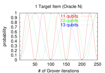
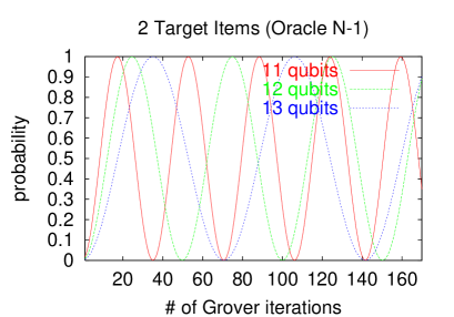
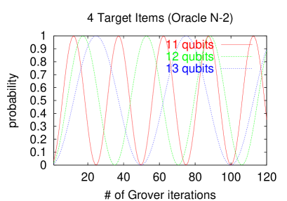
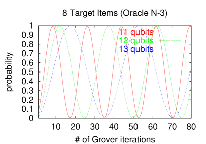
Figure 6: Probability of successful search for one, two, four and eight items as a function of the number of iterations after which the measurement is performed (11, 12 and 13 qubits).

5 Conclusions and Future Work

We believe that QuIDDs provide a practical and highly efficient approach to high-performance quantum computational simulation. Their key advantage over straightforward matrix-based simulations is much faster execution and lower memory usage. We developped new software package, QuIDD Pro, for high-performance simulation of quantum circuits. To this end, we simulated Grover’s search algorithm by performing respective gate operations in QuIDD Pro. Our results indicate that QuIDD Pro achieves exponential memory savings compared to MATLAB and other competitors. Additionally, QuiDD Pro was asymptotically faster than competing simulators, however not quite as fast as Grover’s algorithm. Empirically, QuIDD Pro spends on the order of $1.66^{q}$ time searching a system with $q$ qubits. Grover’s search executed on a quantum computer requires time on the order of $\sqrt{2^{q}}\approx 1.41^{q}$, not counting various potential overhead. Since MATLAB-based simulations explicitly store large matrices, their space complexity must be $\Omega(4^{q})$, and the same is true for time complexity because every matrix element is computed and used. Simulations using Blitz++ required $\Theta(2^{q})$ memory which was dominated by the dense state-vector, and their runtime must grow at least as fast. Yet, the simulation using QuIDD Pro required only a linearly-growing amount of memory.

We note that in our experiments, numerical precision of complex-valued terminals was fixed. QuiDDPro currently incorporates variable-precision integer and floating-point number types, and all reported experiments were performed with sufficient numerical precisious to avoid round-off errors. However, we have not yet experimented with precision requirements at larger number of qubits and the effects of round-off errors on our simulations. That will be addressed in our future work that also includes simulating other quantum algorithms, such as Shor’s [16], and modelling the effects of errors and decoherence in quantum computation.

References

- [1] R. Bryant, “Graph-Based Algorithms for Boolean Function Manipulation”, IEEE Trans. on Computers, vol. C-35, pp. 677-691, Aug 1986.
- [2] E. Clarke et al., Multi-Terminal Binary Decision Diagrams and Hybrid Decision Diagrams, In T. Sasao and M. Fujita, eds, Representations of Discrete Functions, pp. 93-108, Kluwer, 1996.
- [3] R. I. Bahar et al., “Algebraic Decision Diagrams and their Applications”, In Proc. IEEE/ACM ICCAD 1993, pp. 188-191, ‘93.
- [4] R. P. Feynman, R. W. Allen and A. J. G. Hey, eds.: “Feynman Lectures on Computation”, Perseus Books, 2000, p. 320.
-
[5]
D. Greve, “QDD: A Quantum Computer Emulation Library”, 1999
http://home.plutonium.net/~dagreve/qdd.html - [6] G. H. Golub and C. F. Van Loan, “Matrix Computations”, 3rd ed., 693 p. Johns Hopkins Univ. Press, 1996.
- [7] D. Gottesman, “The Heisenberg Representation of Quantum Computers”, Plenary speech at the 1998 International Conference on Group Theoretic Methods in Physics, http://arxiv.org/abs/quant-ph/9807006.
- [8] L. Grover, “Quantum Mechanics Helps In Searching For a Needle in a Haystack”, Phys. Rev. Lett. 79 (1997) p. 325.
- [9] A. J. G. Hey, ed.: “Feynman and Computation: Exploring The Limits of Computers”, Perseus Books, 1999, p. 438.
- [10] D. Long, “A BDD Library With Modifications For Sequential Verification”, 1993 http://www-2.cs.cmu.edu/~modelcheck/bdd.html
- [11] M. Boyer, G. Brassard, P. Hoyer, Alain Tapp, “Tight Bounds on Quantum Searching”, Fourth Workshop on Physics and Computation, Boston, Nov. 1996.
- [12] “Efforts to Transform Computers Reach a Milestone”, New York Times, December 20, 2001.
- [13] M. A. Nielsen and I. L. Chuang, “Quantum Computation and Quantum Information”, ch. 2,4,5, and 6, Cambridge Univ. Press, 2000, 675 pages.
- [14] G. Hachtel et al., “Markovian Analysis of Large Finite State Machines”, IEEE Trans. on Computer-Aided Design Vol. 15, pp. 1479-1493, Dec. 1996.
- [15] S. O’uchi, M. Fujishima and H. Koichiro, ”An 8-qubit quantum-circuit processor”, in Proc. 2002 IEEE International Symposium on Circuits and Systems, vol. 5, pp. 209 -212.
- [16] P. W. Shor, “Polynomial-time Algorithms For Prime Factorization and Discrete Logarithms on a Quantum Computers”, SIAM J. Computing 26 (1997) p. 1484.
- [17] F. Somenzi, “CUDD: CU Decision Diagram Package”, release 2.3.0 Univ. of Colorado at Boulder, 1998. http://vlsi.Colorado.EDU/~fabio/CUDD/
- [18] T. Veldhuizen, “Arrays in Blitz++”, in Proc. 2nd Intl. Symp. on Computing in OO Parallel Environments, 1998. http://www.oonumerics.org/blitz/
- [19] J. Wallace, “Quantum Computer Simulators” CASYS, Intl. J. of Computing Anticipatory Syst., Vol. 10, pp. 230-245; CHAOS 2000.
- [20] C, Zalka, “Simulating Quantum Systems on a Quantum Computer” Proc. Royal Soc. A, Vol. 454, pp. 313-322, Jan. 1998. http://xxx.lanl.gov/abs/quant-ph/9603026