Computational Model for the One-Way Quantum Computer:
Concepts and Summary

Abstract

The one-way quantum computer ($\mbox{QC}_{\cal{C}}$) is a universal scheme of quantum computation consisting only of one-qubit measurements on a particular entangled multi-qubit state, the cluster state. The computational model underlying the $\mbox{QC}_{\cal{C}}\,\,$is different from the quantum logic network model and it is based on different constituents. It has no quantum register and does not consist of quantum gates. The $\mbox{QC}_{\cal{C}}\,\,$is nevertheless quantum mechanical since it uses a highly entangled cluster state as the central physical resource. The scheme works by measuring quantum correlations of the universal cluster state.

I Introduction

Quantum computational models play a twofold role in the development of quantum information science. On the theoretical side, they provide the framework in which mathematical concepts such as a “computation” or an “algorithmic procedure” become connected to the laws of physics. Basic notions of computer science such as “computational complexity” or ‘logical depth” are usually derived with reference to such a model. On the practical side, computational models can have a strong influence on the design of actual experiments that try to realize a quantum computer in the laboratory.

The first model of a quantum computer, the quantum Turing machine (QTM) introduced by Deutsch QTM and further developed by Bernstein and Vazirani BV , connects a computation to a unitary transformation on the Hilbert space spanned by all possible “configurations” of the machine. Unlike its classical analog, it can be in a coherent superposition of many different configurations at the same time, which allows for the interference of different computational paths during a computation. This distinct feature of the QTM has opened the room for the invention of more efficient (quantum) algorithms that make use of interference effects.

On the other hand, most proposals for implementing a quantum computer in real physical systems do not follow the model of a quantum Turing machine. The design of most of todays experiments follow instead the model of a quantum logic network (QLN) QLNW ,Yao . Although it was shown to be computationally equivalent to the QTM QLNW ,Yao , this model has been used more commonly in both theoretical and experimental investigations. The notion of quantum gates makes it much simpler to formulate quantum algorithms in the network language and most of the quantum algorithms that one knows of today –including Shor’s celebrated factoring algorithm fac – have been formulated within the network model. Furthermore, the fact that universal sets of quantum gates can be realized from only two-qubit interactions barenco95 has considerably simplified the problem of identifying specific physical systems that are suitable DiV for quantum computation.

In both the QTM and the QLN model of a quantum computer, unitary evolution plays a key role, even though the way how such a unitary evolution is generated is quite different. Recently, it has become clear that quantum gates (and thus general unitary transformations) need not be generated from a coherent Hamiltonian dynamics. Instead several schemes QFT -Nil have been proposed in which projective von Neumann measurements play a constitutive role.

Recently, we introduced the scheme of the one-way quantum computer QCmeas . This scheme uses a given entangled state, the so-called cluster state BR , as its central physical resource. The entire quantum computation consists only of a sequence one-qubit projective measurements on this entangled state. We called this scheme the “one-way quantum computer” since the entanglement in the cluster state is destroyed by the one-qubit measurements and therefore it can only be used once. While it is possible to simulate any unitary evolution with the one-way quantum computer, the computational model of the $\mbox{QC}_{\cal{C}}\,\,$makes no reference to the concept of unitary evolution. A quantum computation corresponds, instead, to a sequence of simple projections in the Hilbert space of the cluster state. The information that is processed is extracted from the measurement outcomes and is thus a purely classical quantity.

As we have shown in QCmeas , any quantum logic network can be simulated efficiently on the one-way quantum computer. This shows that the one-way quantum computer is, in fact, universal. Surprisingly, it turns out that for many algorithms the simulation of a unitary network can be parallelized to a higher degree than the original network itself. As an example, circuits in the Clifford group –which is generated by the CNOT-gates, Hadamard-gates and $\pi/2$-phase shifts– can be performed by a $\mbox{QC}_{\cal{C}}\,\,$in a single time step, i.e. all the measurements to implement such a circuit can be carried out at the same time. More generally, in a simulation of a quantum logic network by a one-way quantum computer, the temporal ordering of the gates of the network is transformed into a spatial pattern of measurement bases for the individual qubits on the resource cluster state. For the temporal ordering of the measurements there is, however, no counterpart in the network model. Therefore, the question of complexity of a quantum computation must be possibly revisited.

In the following we would like to give an introduction to the computational model that describes information processing with the one-way quantum computer. To stress the importance of the cluster state for the scheme, we will use the abbreviation QC_C for “one-way quantum computer”. The computational model underlying the QC_C has been described in a technical report in Ref. model . The purpose of the present paper is to give a summary of this model, concentrating on the concepts that we have introduced to describe computation with the $\mbox{QC}_{\cal{C}}$. We describe the objects that comprise the information processed with the $\mbox{QC}_{\cal{C}}\,\,$and the temporal structure of this processing. The reader who is interested in the details of the derivations is referred to model .

II The $\mbox{QC}_{\cal{C}}\,\,$as a universal simulator of quantum logic networks

In this section, we give an outline of the universality proof QCmeas for the $\mbox{QC}_{\cal{C}}$. To demonstrate universality we show that the $\mbox{QC}_{\cal{C}}\,\,$can simulate any quantum logic network efficiently. It shall be pointed out from the beginning that the network model does not provide the most suitable description for the $\mbox{QC}_{\cal{C}}$. Nevertheless, the network model is the most widely used form of describing a quantum computer and therefore the relation between the network model and the $\mbox{QC}_{\cal{C}}\,\,$must be clarified.

For the one-way quantum computer, the entire resource for the quantum computation is provided initially in the form of a specific entangled state –the cluster state BR – of a large number of qubits. Information is then written onto the cluster, processed, and read out from the cluster by one-particle measurements only. The entangled state of the cluster thereby serves as a universal “substrate” for any quantum computation. Cluster states can be created efficiently in any system with a quantum Ising-type interaction (at very low temperatures) between two-state particles in a lattice configuration. More specifically, to create a cluster state $|\phi\rangle_{\cal{C}}$, the qubits on a cluster ${\cal{C}}$ are at first all prepared individually in a state $|+\rangle=1/\sqrt{2}(|0\rangle+|1\rangle)$ and then brought into a cluster state by switching on the Ising-type interaction $H_{\mbox{\tiny{int}}}$ for an appropriately chosen finite time span $T$. The time evolution operator generated by this Hamiltonian which takes the initial product state to the cluster state is denoted by $S$.

The quantum state $|\phi\rangle_{\cal{C}}$, the cluster state of a cluster $\cal C$ of neighbouring qubits, provides in advance all entanglement that is involved in the subsequent quantum computation. It has been shown BR that the cluster state $|\phi\rangle_{\cal C}$ is characterized by a set of eigenvalue equations

$$\sigma_{x}^{(a)}\bigotimes_{a^{\prime}\in ngbh(a)}\sigma_{z}^{(a^{\prime})}|\phi\rangle_{\cal C}={(-1})^{\kappa_{i}}|\phi\rangle_{\cal C},$$ (1)

where $ngbh(a)$ specifies the sites of all qubits that interact with the qubit at site $a\in{\cal C}$ and $\kappa_{i}\in\{0,1\}$ for all $i\in{\cal{C}}$. The equations (1) are central for the proposed computation scheme. Cluster states specified by different sets $\{\kappa_{i},i\in{\cal{C}}\}$ are local unitary equivalent, i.e. can be transformed into each other by local unitary rotations of single qubits, and are thus equally good for computation. In the following we will therefore confine ourselves to the case of

$$\kappa_{i}=0\,\;\forall i\in{\cal{C}}.$$ (2)

It is important to realize here that information processing is possible even though the result of every measurement in any direction of the Bloch sphere is completely random. The reason for the randomness of the measurement results is that the reduced density operator for each qubit in the cluster state is $\frac{1}{2}{\bf{1}}$. While the individual measurement results are irrelevant for the computation, the strict correlations between measurement results inferred from (1) are what makes the processing of quantum information on the $\mbox{QC}_{\cal{C}}\,\,$possible.

For clarity, let us emphasize that in the scheme of the $\mbox{QC}_{\cal{C}}\,\,$we distinguish between cluster qubits on ${\cal{C}}$ which are measured in the process of computation, and the logical qubits. The logical qubits constitute the quantum information being processed while the cluster qubits in the initial cluster state form an entanglement resource. Measurements of their individual one-qubit state drive the computation.

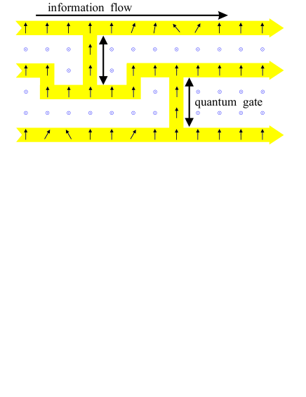
Figure 1: Simulation of a quantum logic network by measuring two-state particles on a lattice. Before the measurements the qubits are in the cluster state $|\phi\rangle_{\cal{C}}$ of (1). Circles $\odot$ symbolize measurements of $\sigma_{z}$, vertical arrows are measurements of $\sigma_{x}$, while tilted arrows refer to measurements in the x-y-plane.

To process quantum information with this cluster, it suffices to measure its particles in a certain order and in a certain basis, as depicted in Fig. 1. Quantum information is thereby propagated through the cluster and processed. Measurements of $\sigma_{z}$-observables effectively remove the respective lattice qubit from the cluster. Measurements in the $\sigma_{x}$- (and $\sigma_{y}$-) eigenbasis are used for “wires”, i.e. to propagate logical quantum bits through the cluster, and for the CNOT-gate between two logical qubits. Observables of the form $\cos(\varphi)\,\sigma_{x}\pm\sin(\varphi)\,\sigma_{y}$ are measured to realize arbitrary rotations of logical qubits. For these cluster qubits, the basis in which each of them is measured depends on the results of preceding measurements. This introduces a temporal order in which the measurements have to be performed. The processing is finished once all qubits except a last one on each wire have been measured. The remaining unmeasured qubits form the quantum register which is now ready to be read out. At this point, the results of previous measurements determine in which basis these “output” qubits need to be measured for the final readout, or if the readout measurements are in the $\sigma_{x}$-, $\sigma_{y}$- or $\sigma_{z}$-eigenbasis, how the readout measurements have to be interpreted. Without loss of generality, we assume in this paper that the readout measurements are performed in the $\sigma_{z}$-eigenbasis.

To understand the $\mbox{QC}_{\cal{C}}\,\,$in network model terms, in the same way as we decompose networks into gates, we would like to decompose a $\mbox{QC}_{\cal{C}}$-circuit as a simulator of a quantum logic network into simulations of quantum gates. This requires some adaption. First of all, we need to identify a quantum input and -output. To do so, we first modify the $\mbox{QC}_{\cal{C}}$-computation slightly and later remove this modification again. The modification is this: instead of creating a universal cluster state and subsequently measuring it we now allow for read-in of an arbitrary quantum input. Then, the modified procedure consists of the following steps. 1) Prepare a state $|\psi_{\mbox{\footnotesize{in}}}\rangle_{I}\otimes(\bigotimes_{j\in{\cal{C}}\backslash I}|+\rangle_{j})$ where $|\psi_{\mbox{\footnotesize{in}}}\rangle$ is the input state prepared on a subset of the cluster qubits $I\subset{\cal{C}}$. 2) Entangle the state via the unitary evolution $S$ generated by the Ising interaction. 3a) Measure all cluster qubits except for those of the output register $O\subset{\cal{C}}$. In this way, the state $|\psi_{\mbox{\footnotesize{in}}}\rangle$ is teleported from $I$ to $O$ and at the same time processed. 3b) Measure the qubits in the output register $O$ (readout).

Please note that for the “default input” $|\psi_{\mbox{\footnotesize{in}}}\rangle_{I}=\bigotimes_{i\in I}|+\rangle_{i}$ this modified procedure is equivalent to the original one. Then, steps 1 and 2 create a cluster state (which could as well be created by any other method) and steps 3a) and 3b) form the sequence of measurements. As will be discussed in Section III, as long as the quantum input is known it is sufficient to consider $\bigotimes_{i\in I}|+\rangle_{i}$ and thus one-qubit measurements on cluster states.

Steps 1) - 3a) form the procedure to simulate some unitary network applied to the quantum register. It is decomposed into similar sub-procedures for gate simulation: loading the input, entangling operation, measurement of all but the output qubits. Provided the measurement bases have been chosen appropriately, a procedure of this type teleports a general input state from one part of the cluster to another and thereby also processes it.

We explain the $\mbox{QC}_{\cal{C}}\,\,$as a succession of gate simulations, i.e. as repeated steps of entangling operations and measurements on sub-clusters. In reality, however, a different scheme is realized, namely first all the cluster qubits are entangled and second they are measured. These to ways to proceed are mathematically equivalent as has been demonstrated in QCmeas . The basic reason for this equivalence is that, in the sequential picture, later entangling operations commute with earlier measurements because they act on different particles. Therefore, the order of operations can be interchanged such that first all entangling operations and after that all measurements are performed.

In the following we review two points of the universality proof for the $\mbox{QC}_{\cal{C}}$: the realization of the arbitrary one-qubit rotation as a member of the universal set of gates, and the effect of the randomness of the individual measurement results and how to account for them. For the realization of a CNOT-gate see Fig. 2 and QCmeas .

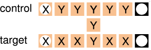
CNOT-gate
Hadamard-gate	$\pi/2$-phase gate
rotation

Figure 2: Realization of the required gates on the $\mbox{QC}_{\cal{C}}$. CNOT-gate between neighbouring qubits, the Hadamard gate, the $\pi/2$ phase gate and the general rotation specified by the three Euler angles $\xi$, $\eta$, $\zeta$.

An arbitrary rotation $U_{R}\in SU(2)$ can be achieved in a chain of 5 qubits. Consider a rotation in its Euler representation

$$U_{R}(\xi,\eta,\zeta)=U_{x}(\zeta)U_{z}(\eta)U_{x}(\xi),$$ (3)

where the rotations about the $x$- and $z$-axis are $U_{x}(\alpha)=\displaystyle{\mbox{exp}\left(-i\alpha\frac{\sigma_{x}}{2}\right)}$ and $U_{z}(\alpha)=\displaystyle{\mbox{exp}\left(-i\alpha\frac{\sigma_{z}}{2}\right)}$. Initially, the first qubit is in some state $|\psi_{\mbox{\footnotesize{in}}}\rangle$, which is to be rotated, and the other qubits are in $|+\rangle$. After the 5 qubits are entangled by the time evolution operator $S$ generated by the Ising-type Hamiltonian, the state $|\psi_{\mbox{\footnotesize{in}}}\rangle$ can be rotated by measuring qubits 1 to 4. At the same time, the state is also transfered to site 5. The qubits $1\dots 4$ are measured in appropriately chosen bases, viz.

$${\cal{B}}_{j}(\varphi_{j})=\left\{\frac{|0\rangle_{j}+e^{i\varphi_{j}}|1\rangle_{j}}{\sqrt{2}},\,\frac{|0\rangle_{j}-e^{i\varphi_{j}}|1\rangle_{j}}{\sqrt{2}}\right\}$$ (4)

whereby the measurement outcomes $s_{j}\in\{0,1\}$ for $j=1\dots 4$ are obtained. Here, $s_{j}=0$ means that qubit $j$ is projected into the first state of ${\cal{B}}_{j}(\varphi_{j})$. In (4) the basis states of all possible measurement bases lie on the equator of the Bloch sphere, i.e. on the intersection of the Bloch sphere with the $x-y$-plane. Therefore, the measurement basis for qubit $j$ can be specified by a single parameter, the measurement angle $\varphi_{j}$. The measurement direction of qubit $j$ is the vector on the Bloch sphere which corresponds to the first state in the measurement basis ${\cal{B}}_{j}(\varphi_{j})$. Thus, the measurement angle $\varphi_{j}$ is equal to the angle between the measurement direction at qubit $j$ and the positive $x$-axis. For all of the gates constructed so far, the cluster qubits are either –if they are not required for the realization of the circuit– measured in $\sigma_{z}$, or –if they are required– measured in some measurement direction in the $x-y$-plane. In summary, the procedure to implement an arbitrary rotation $U_{R}(\xi,\eta,\zeta)$, specified by its Euler angles $\xi,\eta,\zeta$, is this: 1. measure qubit 1 in ${\cal{B}}_{1}(0)$; 2. measure qubit 2 in ${\cal{B}}_{2}\left(-(-1)^{s_{1}}\xi\right)$; 3. measure qubit 3 in ${\cal{B}}_{3}\left(-(-1)^{s_{2}}\eta\right)$; 4. measure qubit 4 in ${\cal{B}}_{4}\left(-(-1)^{s_{1}+s_{3}}\zeta\right)$. In this way the rotation $U_{R}^{\prime}$ is realized:

$$U_{R}^{\prime}(\xi,\eta,\zeta)=U_{\Sigma}U_{R}(\xi,\eta,\zeta).$$ (5)

The random byproduct operator

$$U_{\Sigma}=\sigma_{x}^{s_{2}+s_{4}}\sigma_{z}^{s_{1}+s_{3}}$$ (6)

can be corrected for at the end of the computation, as explained next.

The randomness of the measurement results does not jeopardize the function of the circuit. Depending on the measurement results, extra rotations $\sigma_{x}$ and $\sigma_{z}$ act on the output qubits of every implemented gate, as in (5), for example. By use of the propagation relations

$$\begin{array}[]{l}U_{R}(\xi,\eta,\zeta)\,\sigma_{z}^{s}\sigma_{x}^{s^{\prime}}=\\ \hskip 19.91684pt\sigma_{z}^{s}\sigma_{x}^{s^{\prime}}\,U_{R}((-1)^{s}\xi,(-1)^{s^{\prime}}\eta,(-1)^{s}\zeta),\end{array}$$ (7)

$$\begin{array}[]{l}\mbox{CNOT}(c,t)\,{\sigma_{z}^{(t)}}^{s_{t}}{\sigma_{z}^{(c)}}^{s_{c}}{\sigma_{x}^{(t)}}^{s_{t}^{\prime}}{\sigma_{x}^{(c)}}^{s_{c}^{\prime}}=\\ \hskip 19.91684pt{\sigma_{z}^{(t)}}^{s_{t}}{\sigma_{z}^{(c)}}^{s_{c}+s_{t}}{\sigma_{x}^{(t)}}^{s_{c}^{\prime}+s_{t}^{\prime}}{\sigma_{x}^{(c)}}^{s_{c}^{\prime}}\,\mbox{CNOT}(c,t),\end{array}$$ (8)

these extra rotations can be pulled through the network to act upon the output state. There they can be accounted for by properly interpreting the $\sigma_{z}$-readout measurement results.

The propagation relations for the general rotations and for the CNOT gate, respectively, are different in the following respect. In the propagation relation for the CNOT gate the gate remains unchanged and the byproduct operator is modified. For rotations this is in general not possible if one demands that the byproduct operator must remain in the Pauli group, which is essential. Therefore, in the propagation relations for rotations the gate changes and the byproduct operator remains unmodified. This is the origin of adaptive measurement bases and thus the temporal structure of $\mbox{QC}_{\cal{C}}$-algorithms.

The reason why the propagation relation for the CNOT gate takes the form (8) is that it is in the Clifford group, the normalizer of the Pauli group, which means that a Pauli operator is mapped onto a Pauli operator under conjugation with any Clifford group element. There are also local rotations in the Clifford group, among them the Hadamard transformation and the $\pi/2$-phase gate. These rotations can be simulated more efficiently than by the procedure for general rotations described above. To see this, note that the measurement bases ${\cal{B}}(\varphi)$ and ${\cal{B}}(-\varphi)$ in (4) coincide for angles $\varphi=0$ and for $\varphi=\pm\pi/2$. For $\varphi=0$ the measurement basis ${\cal{B}}(\varphi)$ is the eigenbasis of $\sigma_{x}$, and for $\varphi=\pm\pi/2$ the measurement basis ${\cal{B}}(\varphi)$ is the eigenbasis of $\sigma_{y}$. In these cases, the choice of the measurement basis is not influenced by the results of measurements at other qubits. The Hadamard gate and the $\pi/2$ phase shift are such rotations. As displayed in Fig. 2, they are both realized by performing a pattern of $\sigma_{x}$- and $\sigma_{y}$-measurements on the cluster ${\cal{C}}$. The byproduct operators which are thereby created are

$$\begin{array}[]{rcl}U_{\Sigma,H}&=&\sigma_{x}^{s_{1}+s_{3}+s_{4}}\,\sigma_{z}^{s_{2}+s_{3}}\\ U_{\Sigma,U_{z}(\pi/2)}&=&\sigma_{x}^{s_{2}+s_{4}}\,\sigma_{z}^{s_{1}+s_{2}+s_{3}+1}.\end{array}$$ (9)

Owing to the fact that the Hadamard- and the $\pi/2$-phase gate are in the Clifford group, the propagation relations for these rotations can also be written in a form resembling the propagation relation (8) for the CNOT-gate

$$\begin{array}[]{rcl}H\,{\sigma_{x}}^{s_{x}}{\sigma_{z}}^{s_{z}}&=&{\sigma_{x}}^{s_{z}}{\sigma_{z}}^{s_{x}}\,H,\\ U_{z}(\pi/2)\,{\sigma_{x}}^{s_{x}}{\sigma_{z}}^{s_{z}}&=&{\sigma_{x}}^{s_{x}}{\sigma_{z}}^{s_{x}+s_{z}}\,U_{z}(\pi/2).\end{array}$$ (10)

As stated above, the measurement bases to implement the Hadamard- and the $\pi/2$-phase gate require no adjustment since only operators $\sigma_{x}$ and $\sigma_{y}$ are measured. The same holds for the implementation of the CNOT gate, see Fig. 2. Thus, all the Hadamard-, $\pi/2$-phase- and CNOT-gates of a quantum circuit can be implemented simultaneously in the first measurement round with no regard to their location in the network. In particular, quantum circuits which consist only of such gates, i.e. circuits in the Clifford group, can be realized in a single time step. As an example, many circuits for coding and decoding are in the Clifford group.

The fact that quantum circuits in the Clifford group can be realized in a single time step has previously not been known for networks. The best upper bound on the logical depth known so far scales logarithmically with the number of logical qubits M&N . One might therefore wonder whether the $\mbox{QC}_{\cal{C}}\,\,$is more efficient than a quantum computer realized as a quantum logic network. This is not the case in so far as both the quantum logic network computer and the $\mbox{QC}_{\cal{C}}\,\,$can simulate each other efficiently. The fact that each quantum logic network can be simulated on the $\mbox{QC}_{\cal{C}}\,\,$has been shown in QCmeas . The converse is also true because a resource cluster state of arbitrary size can be created by a quantum logic network of constant logical depth. Furthermore, the subsequent one-qubit measurements are within the set of standard tools employed in the network scheme of computation. In this sense, the operation of the $\mbox{QC}_{\cal{C}}\,\,$can be cast entirely in network language.

However, while the network model comprises the means that are used in a computation on a $\mbox{QC}_{\cal{C}}$, it cannot describe how they have to be used. In particular, in the above construction –where a $\mbox{QC}_{\cal{C}}\,\,$simulating a quantum logic network is itself simulated by a more complicated network– the temporal order of the measurements and the rules to adapt the measurement bases are not provided with the network description. But without this additional information the network to simulate the $\mbox{QC}_{\cal{C}}\,\,$is incomplete.

It should be noted that a link between the degree of parallelization of unitary operations and the logical depth of a quantum algorithm does not exist a priori. It is established only if quantum computation is identified with unitary evolution. The network model allows statements about how much one can parallelize networks composed of unitary gates. As an example, two unitary gates $U_{1}$, $U_{2}$ cannot be performed in parallel if they do not commute. For simulations of such gates with the $\mbox{QC}_{\cal{C}}$, however, this general restriction does not apply: The simulations of two non-commuting gates can still be parallelized if the gates are in the Clifford group.

With this observation we complete the survey of the universality proof QCmeas for the $\mbox{QC}_{\cal{C}}$. To summarize, for simulation of a quantum logic network on a one-way quantum computer, a set of universal gates can be realized by one-qubit measurements and the gates can be combined to circuits. Due to the randomness of the results of the individual measurements, extra byproduct operators occur. These byproduct operators specify how the readout of the simulated quantum register has to be interpreted. Also, they influence the bases of the one-qubit measurements.

In this section we have described the $\mbox{QC}_{\cal{C}}\,\,$as a simulator of quantum logic networks. We adopted all the network notions such as the “quantum register” and “quantum gates”. We have found an additional structure, the byproduct operator, which keeps track of the randomness introduced by the measurements. In a network-like description of the $\mbox{QC}_{\cal{C}}$, the byproduct operator appears as some unwanted extra complication that has to be and fortunately can be handled. In the next section we will point out in which respect the description of the $\mbox{QC}_{\cal{C}}\,\,$as a network simulator is not adequate and in Section IV we will present a different computational model for the $\mbox{QC}_{\cal{C}}$. For this model it will turn out that the byproduct operators form, in fact, the central quantities of information processing with the $\mbox{QC}_{\cal{C}}$, and that the “quantum register” and the “quantum gates” disappear.

III Non-network character of the $\mbox{QC}_{\cal{C}}\,\,$

In the network model of quantum computation one usually regards the state of a quantum register as the carrier of information. The quantum register is prepared in some input state and processed to some output state by applying a suitable unitary transformation composed of quantum gates. Finally, the output state of the quantum register is measured by which the classical readout is obtained.

In this section we explain why the notions of “quantum input” and “quantum output” have no genuine meaning for the $\mbox{QC}_{\cal{C}}\,\,$if we restrict ourselves to the situation where the quantum input state is known. Shor’s factoring algorithm fac and Grover’s data base search algorithm searoot are both examples of such a situation. In these algorithms one always starts with the input state $\bigotimes_{i=1}^{n}1/\sqrt{2}(|0\rangle_{i}+|1\rangle_{i})=|++...+\rangle$. Other scenarios are conceivable, e.g. where an unknown quantum input is processed and the classical result of the computation is retransmitted to the sender of the input state; or the unmeasured network output register state is retransmitted. These scenarios would lead only to minor modifications in the computational model. How to process an unknown quantum state has been briefly discussed in Section II but is not in the focus of this paper. So, let us assume that the quantum input is known. There it is sufficient to discuss the situation where an input state $|++..+\rangle_{I}$ is read in on some subset $I\subset{\cal{C}}$ of the cluster ${\cal{C}}$. Any other known input state can be created on the cluster from the standard quantum state $|++..+\rangle$, by some circuit preceding the main one.

Reading in an input state $\bigotimes_{i\in I}|+\rangle_{i}$ means to prepare the state $S[\bigotimes_{i\in I}|+\rangle_{i}\otimes(\bigotimes_{j\in{\cal{C}}\backslash I}|+\rangle_{j})]=|\phi\rangle_{\cal{C}}$, i.e. to prepare nothing but a cluster state. The cluster state $|\phi\rangle_{\cal{C}}$ is a universal resource, no input dependent information specifies it. In this sense, the $\mbox{QC}_{\cal{C}}\,\,$has no quantum input.

Similarly, the $\mbox{QC}_{\cal{C}}\,\,$has no quantum output. Of course, the final result of any computation –including quantum computations– is a classical number, but for the quantum logic network the state of the output register before the readout measurements plays a distinguished role. For the $\mbox{QC}_{\cal{C}}\,\,$this is not the case, there are just cluster qubits measured in a certain order and basis. The measurement outcomes contribute all to the result of the computation.

We have identified subsets $I$, $O$ on the cluster ${\cal{C}}$ –$I$ for the subset of the cluster which simulates the quantum register in its input state and $O$ to simulate the quantum register in its output state– only to make the $\mbox{QC}_{\cal{C}}\,\,$suitable for a description in terms of the network model. Such a terminology is not required for the $\mbox{QC}_{\cal{C}}\,\,$a priori. It is not even appropriate: if, to perform a particular algorithm on the $\mbox{QC}_{\cal{C}}$, a quantum logic network is implemented on a cluster state there is a subset of cluster qubits which play the role of the output register. These qubits are not the final ones to be measured, but among the first (!).

As we have seen, the measurement outcomes from all the cluster qubits contribute to the result of the computation. The qubits from $O\subset{\cal{C}}$ simulate the output state of the quantum register and thus contribute directly. The cluster qubits in the set $I\subset{\cal{C}}$ simulate the input state of the quantum register and the outcomes obtained in their measurement contribute via the accumulated byproduct operator that is required to interpret the readout measurements on $O$. Finally, the qubits in the section $M\subset{\cal{C}}$ of the cluster by whose measurements the quantum gates are simulated also contribute via the byproduct operator.

Naturally there arises the question whether there is any difference in the way how measurements of cluster qubits in $I$, $O$ or $M$ contribute to the final result of the computation. As shown in model , it turns out that there is none. This is why we abandon the notions of quantum input and quantum output altogether from the description of the $\mbox{QC}_{\cal{C}}$.

IV Computational model

Quantum gates are not constitutive elements of the $\mbox{QC}_{\cal{C}}$; these are instead one-qubit measurements performed in a certain temporal order and in a spatial pattern of adaptive measurement bases. The most efficient temporal order of the measurements does not follow from the temporal order of the simulated gates in the network model. Therefore, a set of rules is required by which the optimal order of measurements can be inferred. Generally, for circuits which involve a vast number of measurements and subsequent conditional processing, it becomes essential to have an additional structure to process the classical information gained by the measurements. The $\mbox{QC}_{\cal{C}}\,\,$provides such a structure - the information flow vector ${\bf{I}}(t)$ (see model and below). In fact, for the computational model of the $\mbox{QC}_{\cal{C}}\,\,$this classical binary-valued quantity will turn out to be the central object for information processing.

So let us take a step back and look what the $\mbox{QC}_{\cal{C}}\,\,$is. On the quantum level, the $\mbox{QC}_{\cal{C}}\,\,$works by measuring quantum correlations of the initial universal cluster state. With the creation of the universal cluster state these quantum correlations are provided before the computation starts. In contrast to the network model, they are not created in a procedure specific to the computational problem. Therefore, for the $\mbox{QC}_{\cal{C}}\,\,$there is no processing of information on the quantum level. In this sense, besides no quantum input and no quantum output, the $\mbox{QC}_{\cal{C}}\,\,$has no quantum register either.

Central from the conceptual point of view but also vital for the practical realizability of the scheme is that the quantum correlations of the cluster state can be measured qubit-wise. This requires a temporal ordering of the measurements and adaptive measurement bases in accordance with previously obtained measurement results. Thus there is processing at the classical level.

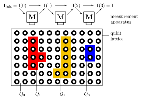
Figure 3: General scheme of the quantum computer via one-qubit measurements. The sets $Q_{t}$ of lattice qubits are measured one after the other. The results of earlier measurements determine the measurement bases of later ones. All classical information from the measurement results needed to steer the $\mbox{QC}_{\cal{C}}\,\,$is contained in the information flow vector ${\bf{I}}(t)$. After the last measurement round $t_{\mbox{\footnotesize{max}}}$, ${\bf{I}}(t_{\mbox{\footnotesize{max}}})$ contains the result of the computation.

The general view of a $\mbox{QC}_{\cal{C}}$-computation is as follows. The cluster ${\cal{C}}$ is divided into disjoint subsets $Q_{t}\subset{\cal{C}}$ with $0\leq t\leq t_{\mbox{\footnotesize{max}}}$, i.e. $\bigcup_{t=0}^{t_{\mbox{\tiny{max}}}}Q_{t}={\cal{C}}$ and $Q_{s}\cap Q_{t}=\emptyset$ for all $s\not=t$. The cluster qubits within each set $Q_{t}$ can be measured simultaneously and the sets are measured one after another. The set $Q_{0}$ consists of all those qubits of which no measurement bases have to be adjusted, i.e. those of which the operator $\sigma_{x}$, $\sigma_{y}$ or $\sigma_{z}$ is measured. This comprises all the redundant qubits, the qubits to implement the Clifford part of the circuit and the qubits which simulate the network quantum output. In the subsequent measurement rounds only operators of the form $\cos\varphi\,\sigma_{x}+\pm\sin\varphi\,\sigma_{y}$ are measured where $|\varphi|<\pi/2$, $\varphi\neq 0$. The measurement bases are adaptive in these rounds. The measurement outcomes from the qubits in $Q_{0}$ specify the measurement bases for the qubits in $Q_{1}$ which are measured in the second round, those from $Q_{0}$ and $Q_{1}$ together specify the bases for the measurements of the qubits in $Q_{2}$ which are measured in the third round, and so on. Finally, the result of the computation is calculated from the measurement outcomes in all the measurement rounds.

Now there arise two questions. First, “Given a quantum algorithm, how can one find the measurement pattern and in particular the temporal order in which the measurements are performed?”. As for the measurement pattern, apart from a few exceptions such as the quantum Fourier transformation or the quantum adding circuit LongMeas presently we know no better than to straightforwardly simulate the network. Even then the optimal temporal order of the measurements is, as stated before, different from what one expects from the order of gates in the quantum logic network. The discussion of temporal complexity within the $\mbox{QC}_{\cal{C}}\,\,$will lead us to objects such as the forward cones, the byproduct images and the information flow vector model which will be briefly introduced below. The second question is: “How complicated is the required classical processing?”. In principle it could be that all the obtained measurement results had to be stored separately and the functions to compute the measurement bases were so complicated that one would gain no advantage over the classical algorithm for the considered problem. This is not at all the case. If the network algorithm runs on $n$ qubits then the classical data that the $\mbox{QC}_{\cal{C}}\,\,$has to keep track of is all contained in a $2n$-component binary valued vector, the information flow vector ${\bf{I}}(t)$. The update of ${\bf{I}}(t)$, the calculation to adapt the measurement bases of cluster qubits according to previous measurement outcomes and the final identification of the computational result are all elementary.

Let us first discuss the temporal ordering of the measurements. To understand how the sets $Q_{t}$ of simultaneously measurable qubits are constructed we introduce the notion of forward cones. The forward cone $\mbox{fc}(k)$ of a cluster qubit $k\in{\cal{C}}$ is the set of all those cluster qubits $j\in{\cal{C}}$ whose measurement basis ${\cal{B}}(\varphi_{j,\mbox{\footnotesize{meas}}})$ depends on the result $s_{k}$ of the measurement of qubit $k$ after the byproduct operator ${\left(U_{k}\right)}^{s_{k}}$ is propagated forward from the output side of the gate for whose implementation the cluster qubit was measured to the output side of the network. See Fig. 4. Similarly, the backward cone $\mbox{bc}(k)$ of a cluster qubit $k\in{\cal{C}}$ whose measurement bases depend upon the measurement result at qubit $k$ when the byproduct operator is propagated backward to the input side of the network. The method to calculate the forward and backward cones follows immediately from their definitions. Quite surprisingly, it will turn out that only backward cones will appear in the computational model that finally emerges. Nevertheless, the forward cones are used to identify the sets of simultaneously measurable qubits as is explained below.

What does it mean that a cluster qubit $j$ is in the forward cone of another cluster qubit $k$, $j\in\mbox{fc}(k)$? According to the definition, a byproduct operator created via the measurement at cluster qubit $k$ influences the measurement angle $\varphi_{j,\mbox{\footnotesize{meas}}}$ at cluster qubit $j$. To determine the measurement angle at $j$ one must thus wait for the measurement result at $k$. Therefore, the forward cones generate a temporal ordering among the measurements. If $j\in\mbox{fc}(k)$, the measurement at qubit $j$ is performed later than that at qubit $k$. This we denote by $k\prec j$

$$j\in\mbox{fc}(k)\Rightarrow k\prec j.$$ (11)

The relation “$\prec$” is a strict partial ordering, i.e. it is transitive and anti-reflexive. Anti-reflexivity is required for the scheme to be deterministic. Transitivity we use to generate “$\prec$” from the forward cones. This partial ordering can now be used to construct the sets $Q_{t}\subset{\cal{C}}$ of cluster qubits measured in measurement round $t$. Be $Q^{(t)}\subset{\cal{C}}$ the set of qubits which are to be measured in the measurement round $t$ and all subsequent rounds. Then, $Q_{0}$ is the set of qubits which are measured in the first round. These are the qubits of which the observables $\sigma_{x}$, $\sigma_{y}$ or $\sigma_{z}$ are measured, so that the measurement bases are not influenced by other measurement results. Further, $Q^{(0)}={\cal{C}}$. Now, the sequence of sets $Q_{t}$ can be constructed using the following recursion relation

$$\begin{array}[]{lcl}Q_{t}&=&\displaystyle{\left\{q\in Q^{(t)}|\neg\exists p\in{Q}^{(t)}:p\prec q\right\}}\\ Q^{(t+1)}&=&\displaystyle{Q^{(t)}\backslash Q_{t}}.\end{array}$$ (12)

All those qubits which have no precursors in some remaining set $Q^{(t)}$ and thus do not have to wait for results of measurements of qubits in $Q^{(t)}$ are taken out of this set to form $Q_{t}$. The recursion proceeds until ${Q}^{(t_{\mbox{\footnotesize{max}}}+1)}=\emptyset$ for some maximal value $t_{\mbox{\footnotesize{max}}}$ of $t$.

Let us now discuss the classical processing. The scheme that emerges is the following: The classical information gained by the measurements is processed within a flow scheme. The flow quantity is a classical $2n$-component binary vector ${\bf{I}}(t)$, where $n$ is the number of logical qubits of a corresponding quantum logic network and $t$ the number of the measurement round. This vector ${\bf{I}}(t)$, the information flow vector, is updated after every measurement round. That is, after the one-qubit measurements of all qubits of a set $Q_{t}$ have been performed simultaneously, ${\bf{I}}(t-1$) is updated to ${\bf{I}}(t)$ through the results of these measurements. In turn, ${\bf{I}}(t)$ determines which one-qubit observables are to be measured of the qubits of the set $Q_{t+1}$. The result of the computation is given by the information flow vector ${\bf{I}}(t_{\mbox{\footnotesize{max}}})$ after the last measurement round. From this quantity the result of the readout measurement on the quantum register in the corresponding quantum logic network can be read off directly without further processing.

In the following we briefly explain how this model arises. We already mentioned the accumulated byproduct operator $U_{\Sigma}|_{\Omega}$ which is the product of all the $(U_{\Sigma,k})^{s_{k}}$, the forward propagated byproduct operators randomly created by the measurement of qubits $k$ with outcome $s_{k}$. $U_{\Sigma}|_{\Omega}$ determines how the readout has to be interpreted. Now note that the readout measurement results can themselves be expressed in terms of a byproduct operator. Let the quantum register be in the state $|\psi_{\mbox{\footnotesize{out}}}\rangle=\bigotimes_{i\in O}|s_{i}\rangle_{i,z}$ after readout. Then $|\psi_{\mbox{\footnotesize{out}}}\rangle$ can be written as $|\psi_{\mbox{\footnotesize{out}}}\rangle=U_{R}\,\bigotimes_{i\in O}|0\rangle_{i}$ with $U_{R}=\bigotimes_{i\in O}(\sigma_{x}^{(i)})^{s_{i}}$, i.e. as a byproduct operator $U_{R}$ acting on some standard state $|0\rangle_{O}$. This standard state contains no information and can henceforth be discarded. The result of the computation is contained in the byproduct operators. It can be directly read off from the $x$-part of the operator $U_{\Sigma,R}|_{\Omega}=U_{\Sigma}|_{\Omega}U_{R}$.

If one discards the sign of these Pauli operators –an unphysical global phase– they can be mapped onto elements of a $2n$-dimensional discrete vector space ${\cal{V}}$. For this we use the isomorphism

$${\cal{I}}:\,\,I\in{\cal{V}}\longrightarrow{\cal{P}}/\{\pm 1\}\ni U=\prod\limits_{i=1}^{n}\,\,{\left(\sigma_{x}^{(i)}\right)}^{{[I_{x}]}_{i}}{\left(\sigma_{z}^{(i)}\right)}^{{[I_{z}]}_{i}},$$ (13)

where ${[I_{x}]}_{i},{[I_{z}]}_{i}\in\{0,1\}$ are the respective components of $I_{x}$, $I_{z}$ and ${\cal{P}}$ denotes the Pauli group. In particular, the $x$-part of ${\bf{I}}={\cal{I}}^{-1}(U_{\Sigma,R}|_{\Omega})$ represents the result of the quantum computation, corresponding to the readout in the network model.

To establish the terminology in which the classical information processing with the $\mbox{QC}_{\cal{C}}\,\,$is described, we introduce the byproduct images and the symplectic scalar product. The byproduct image ${\bf{F}}_{k}$ of a cluster qubit $k\in{\cal{C}}$ is defined as ${\bf{F}}_{k}={\cal{I}}^{-1}(U_{\Sigma,k}|_{\Omega})$. Note that in the byproduct operators for the implementation of the CNOT- and the $\pi/2$-phase gate there are additional contributions which do not depend upon measurement results, i.e. the byproduct operators are not the identity for all measurement results being zero. These additional byproduct operators have their byproduct images as well. Since they cannot be related to a particular cluster qubit we attribute them to the gate $g$ by whose implementation they are introduced and denote them by ${\bf{F}}_{g}$.

Byproduct images are easier to manipulate than the forward propagated byproduct operators to which they correspond via ${\cal{I}}$. There hold the relations ${\cal{I}}({\bf{F}}_{k}+{\bf{F}}_{l})=\pm{\cal{I}}({\bf{F}}_{k}){\cal{I}}({\bf{F}}_{l})$, ${\cal{I}}(s_{k}{\bf{F}}_{k})=\pm{({\cal{I}}({\bf{F}}_{k}))}^{s_{k}}$. The symplectic scalar product of two byproduct images ${\bf{F}}_{k}$, ${\bf{F}}_{l}$ is defined as

$$({\bf{F}}_{k},{\bf{F}}_{l})_{S}={\bf{F}}_{k,x}^{T}{\bf{F}}_{l,z}+{\bf{F}}_{k,z}^{T}{\bf{F}}_{l,x}\;\mbox{mod}\,2.$$ (14)

It is invariant under the Clifford group. A first application of the objects introduced above is the cone test model ,

$$\forall\;k\in{\cal{C}},j\in Q^{(1)}:j\in\mbox{fc}(k)\vee j\in\mbox{bc}(k)\Leftrightarrow({\bf{F}}_{j},{\bf{F}}_{k})_{S}=1.$$ (15)

Whether a qubit lies in some other qubits backward or forward cone can be read off from the respective byproduct images.

Figure 4: Forward and backward cones. The measurement of a cluster qubit $k$ for the implementation of the shown quantum logic network may, depending on the measurement outcome, result in a byproduct operator $\sigma_{z}$ (the underlying cluster and measurement pattern is not shown). This byproduct operator is propagated forward to act upon the output register as $U_{\Sigma,k}|_{\Omega}$. In forward propagation, it flips the measurement angles of the cluster qubits $m$, $n$ by whose measurement one-qubit rotations are implemented. The cluster qubits $m$ and $n$ are thus in the forward cone of $k$, $m,n\in\mbox{fc}(k)$, while $l$ and $o$ are not. Similarly, $i,j\in\mbox{bc}(k)$.

We are now ready to discuss the process of computation. The goal is to collect all the byproduct images weighted with the measurement results, i.e. to finally obtain ${\bf{I}}={\cal{I}}^{-1}(U_{\Sigma,R}|_{\Omega})=\sum_{g}{\bf{F}}_{g}+\sum_{k\in{\cal{C}}}s_{k}{\bf{F}}_{k}$ with all the cluster qubits measured in the correct basis. Before the computation starts we propagate forward all the byproduct operators attributed to the gates since they do not depend on any measurement results. This reverses a number of angles specifying one-qubit rotations in the network to simulate. In this way, we obtain the algorithm angles $\{\varphi^{\mbox{\footnotesize{init}}}_{j,\mbox{\footnotesize{algo}}}\}$ from the network Euler angles. Further we collect the byproduct images of the gates, ${\bf{I}}_{\mbox{\footnotesize{init}}}=\sum_{g}{\bf{F}}_{g}$.

In the first measurement round we measure all the cluster qubits $k\in Q_{0}$ thereby removing the redundant qubits, implementing the Clifford gates of the circuit and measuring the “output register”. This leaves us with byproduct operators scattered all over the place. These byproduct operators we propagate forward and include their byproduct images into the information flow vector at time $t=0$, ${\bf{I}}(0)={\bf{I}}_{\mbox{\footnotesize{init}}}+\sum_{k\in Q_{0}}s_{k}{\bf{F}}_{k}.$ In forward propagation, the byproduct operators reverse some of the algorithm angles. In this way, we update the algorithm angles $\{\varphi^{\mbox{\footnotesize{init}}}_{j,\mbox{\footnotesize{algo}}}\}$ to the modified algorithm angles $\{\varphi^{\mbox{\footnotesize{0}}}_{j,\mbox{\footnotesize{algo}}}\}$, $\varphi^{\mbox{\footnotesize{0}}}_{j,\mbox{\footnotesize{algo}}}={(-1)}^{\eta_{j}}\varphi^{\mbox{\footnotesize{init}}}_{j,\mbox{\footnotesize{algo}}}$ with $\eta_{j}=\sum_{k\in Q_{0}\,|\,j\in\mbox{\footnotesize{fc}}(k)}s_{k}$.

In subsequent measurement rounds we measure cluster qubits in adapted bases. This also produces byproduct operators in the middle of the network to simulate and we propagate them forward as before. The update of ${\bf{I}}(t)$ is just the same as in the first round. We find

$${\bf{I}}(t)={\bf{I}}(t-1)+\sum_{k\in Q_{t}}s_{k}{\bf{F}}_{k}={\bf{I}}_{\mbox{\footnotesize{init}}}+\sum_{k\in\bigcup_{r=0}^{t}Q_{r}}s_{k}{\bf{F}}_{k}.$$ (16)

After the final update, ${\bf{I}}(t_{\mbox{\footnotesize{max}}})={\bf{I}}$ contains the result of the computation in its $x$-part.

As in the first round, the propagation of byproduct operators affects the angles that specify the measurement bases. The update of these angles in all the subsequent measurement rounds could be performed in the same way as in the first round providing one with a complete history $\{\varphi^{\mbox{\footnotesize{t}}}_{j,\mbox{\footnotesize{algo}}}\}$ of adapted angles. It is not necessary to generate and store this bulk of information. We only need to know the adapted angles $\varphi_{j,\mbox{\footnotesize{meas}}}$ at the time when the respective qubits are measured. These measurement angles $\varphi_{j,\mbox{\footnotesize{meas}}}$ can be obtained in a more compact procedure.

This leads to the question which measurement outcomes affect the choice of the measurement basis at qubit $j\in Q_{t},\,\,t>0$. All the measurement outcomes obtained at qubits $k\in{\cal{C}}$ with $j\in\mbox{fc}(k)$ contribute, i.e.

$$\begin{array}[]{rcl}\varphi_{j,\mbox{\footnotesize{meas}}}&=&\varphi^{\mbox{\footnotesize{init}}}_{j,\mbox{\footnotesize{algo}}}\,(-1)^{\sum_{k\in{\cal{C}}\,|\,j\in\mbox{\tiny{\mbox{fc}}}(k)}s_{k}}\\ &=&\varphi^{\mbox{\footnotesize{0}}}_{j,\mbox{\footnotesize{algo}}}\,(-1)^{\sum_{k\in{\cal{C}}\backslash Q_{0}\,|\,j\in\mbox{\tiny{\mbox{fc}}}(k)}s_{k}}.\end{array}$$ (17)

In the second line of (17) we can now simplify the sign factor by use of the cone test (15). First note that the sum over $k\in{\cal{C}}\backslash Q_{0}$ reduces to a sum over $k\in\bigcup_{r=1}^{t-1}Q_{r}$ because otherwise $j\not\in\mbox{fc}(k)$. Then, for $k\in Q_{r},j\in Q_{t}$, $1<r<t$ qubit $j$ may only be in the forward cone of qubit $k$, but never in the backward cone $\mbox{bc}(k)$. Hence, the cone test simplifies to $j\in\mbox{fc}(k)\Longleftrightarrow({\bf{F}}_{j},{\bf{F}}_{k})_{S}=1$ for such qubits, and we obtain $\sum_{k\in{\cal{C}}\backslash Q_{0}\,|\,j\in\mbox{\tiny{\mbox{fc}}}(k)}s_{k}=\sum_{k\in\bigcup_{r=1}^{t-1}Q_{r}}s_{k}({\bf{F}}_{k},{\bf{F}}_{j})_{S}=({\bf{I}}(t-1)-{\bf{I}}(0),{\bf{F}}_{j})_{S}$, and thus

$$\varphi_{j,\mbox{\footnotesize{meas}}}=\varphi^{\prime}_{j,\mbox{\footnotesize{algo}}}\,(-1)^{({\bf{I}}(t-1),{\bf{F}}_{j})_{S}},$$ (18)

with $\varphi^{\prime}_{j,\mbox{\footnotesize{algo}}}=\varphi^{0}_{j,\mbox{\footnotesize{algo}}}\,(-1)^{({\bf{I}}(0),{\bf{F}}_{j})_{S}}$. If one works this out one finds that the angles $\varphi^{\prime}_{j,\mbox{\footnotesize{algo}}}$ are obtained from the corresponding Euler angles of the network by propagating the byproduct operators of the gates and of the qubits measured in the first round backwards to the input side of the network.

To sum up, the $2n$-component binary valued information flow vector represents the information that is processed with the $\mbox{QC}_{\cal{C}}$. Although random in its numerical value after all measurement rounds but the final one, it has a meaning in every step of the computation. The rule for the adaption of measurement bases (18) invokes the random measurement results of qubits $k\in{\cal{C}}\backslash Q_{0}$ only via the information flow vector. The measurement results on qubits $k\in Q_{0}$ are absorbed into the angles $\varphi^{\prime}_{j,\mbox{\footnotesize{algo}}}$ and can be erased after these angles have been set. The angles $\varphi^{\prime}_{j,\mbox{\footnotesize{algo}}}$ remain unchanged in the further course of computation. After the final update at $t=t_{\mbox{\footnotesize{max}}}$, when there are no measurement bases left to adjust, the information flow vector ${\bf{I}}(t_{\mbox{\footnotesize{max}}})$ displays the result of the computation. The update of ${\bf{I}}(t)$ (16) and the rule to adjust the measurement angles (18) are very simple algebraic operations.

V Conclusion

We have reviewed the computational model underlying the one-way quantum computer model , which is very different from the quantum logic network model. The logical depth of certain algorithms is on the $\mbox{QC}_{\cal{C}}\,\,$lower than has so far been known for networks. As an example, on the $\mbox{QC}_{\cal{C}}\,\,$circuits composed of CNOT-, Hadamard- and $\pi/2$-phase gates have unit logical depth, independent of the number of gates or logical qubits. The best bound for networks known previously scales logarithmically. It therefore seems that the question of temporal complexity must be revisited.

The formal description of the $\mbox{QC}_{\cal{C}}\,\,$is based on primitive quantities of which the most important are the sets $Q_{t}\subset{\cal{C}}$ of cluster qubits defining the temporal ordering of measurements on the cluster state, and the binary valued information flow vector ${\bf{I}}(t)$ which is the carrier of the algorithmic information. Much of the terminology that one is familiar with from the network model has been abandoned since in case of the $\mbox{QC}_{\cal{C}}\,\,$no proper meaning can be assigned to these objects. In fact, the $\mbox{QC}_{\cal{C}}\,\,$has no quantum input, no quantum output, no quantum register and it does not consist of quantum gates.

The $\mbox{QC}_{\cal{C}}\,\,$is nevertheless quantum mechanical as it uses a highly entangled cluster state as the central physical resource. It works by measuring quantum correlations of the universal cluster state.

References

- (1) D. Deutsch, Proc. R. Soc. London Ser. A 400, 97 (1985).
- (2) E. Bernstein and U. Vazirani, Proc. of the 25th Annual ACM Symposium on Theory of Computing, 11 (1993).
- (3) D. Deutsch, Proc. R. Soc. London Ser. A 425, 73 (1989).
- (4) A. Yao, Proc. of the 34th Annual IEEE Symposium of Foundations of Computer Science, 352 (1993).
- (5) P. W. Shor, SIAM J. Sci. Statist. Comput. 26, 1484 (1997).
- (6) A. Barenco et al., Phys. Rev. A 52, 3457 (1995).
- (7) D.P. DiVincenzo, Fortschritte der Physik 48, 771 (2000).
- (8) R. B. Griffiths and C.-S. Niu, Phys. Rev. Lett. 76, 3228 (1996).
- (9) M. A. Nielsen and I. L. Chuang, Phys. Rev. Lett. 79, 321 (1997).
- (10) D. Gottesman and I. L. Chuang, Nature (London) 402, 390 (1999).
- (11) R. Raussendorf and H.-J. Briegel, Phys. Rev. Lett. 86, 5188 (2001).
- (12) E. Knill, R. Laflamme and G. J. Milburn, Nature (London) 409, 46 (2001).
- (13) M. A. Nielsen, quant-ph/0108020 (2001); A. Fenner and Y. Zhang, quant-ph/0111077 (2001); D. W. Leung, quant-ph/0111122 (2001).
- (14) H.-J. Briegel and R. Raussendorf, Phys. Rev. Lett. 86, 910 (2001).
- (15) R. Raussendorf and H.-J. Briegel, quant-ph/0108067 (2001). Submitted to Quant. Inf. Comp.
- (16) C. Moore and M. Nilsson, quant-ph/9808027 (1998).
- (17) L. K. Grover, Phys. Rev. Lett. 79, 325 (1997).
- (18) R. Raussendorf, D. E. Browne and H.-J. Briegel, Quantum computation via one-qubit measurements on cluster states. In preparation.