Transient response of a quantum wave to an instantaneous potential step switching

Abstract

The transient response of a stationary state of a quantum particle in a step potential to an instantaneous change in the step height (a simplified model for a sudden bias switch in an electronic semiconductor device) is solved exactly by means of a semianalytical expression. The characteristic times for the transient process up to the new stationary state are identified. A comparison is made between the exact results and an approximate method.

I Introduction

Assume that due to a constant flux of incident quantum particles a stationary scattering state is formed for a given one dimensional potential profile, and that the asymptotic potential level is changed suddenly. A physical realization would be an abrupt change in the bias voltage of an electronic device MH88 ; Frensley90 . The wave will then respond to the potential switch until a new stationary state is attained for any finite position $x$. Obtaining the characteristic time(s) of the transient is clearly of practical interest to determine the transport properties of small mesoscopic structures, but modelling the process by means of a grid discretization of space in a “finite box” is far from simple Frensley90 . The problem is that the boundary conditions at the box edges are not known a priori and involve simultaneous injection to and absorption from the simulation (box) region. Some approximate ways to deal with the transients have been proposed MH88 ; Frensley90 ; RRH91 ; YE95 but, surprisingly, no exact solution has been obtained up to now. Our aim in this paper is to work out an explicit and exact solution of the transition between stationary monochromatic waves due to an abrupt potential switch. While the calculation is performed for simplicity for a step potential that changes the step height suddenly, other potential profiles, e.g., containing square single or double barriers could be treated similarly. Our results are in fact applicable to the outer regions of an arbitrary cut-off potential with different asymptotic levels by inserting the appropriate reflection and transmission amplitudes. The basic trick to find the exact solution is to implement the action of the evolution operator of the new Hamiltonian on the initial state using an integral expression in the complex momentum plane obtained by Hammer, Weber and Zidell HWZ77 .

II Obtention of the exact expression

For a potential step of the form

$$V(x)=-V_{0}\Theta(x),$$ (1)

where $\Theta(x)$ is the step function and $V_{0}>0$, a stationary state incident from the left has the form

$$\psi_{0}(x)=h^{-1/2}\left\{\begin{array}[]{c}e^{iq_{0}x/\hbar}+R_{0}^{l}(q_{0})e^{-iq_{0}x/\hbar},\;x<0\\ T_{0}^{l}(q_{0})e^{ip_{0}x/\hbar},\;x\geq 0\end{array}\right.$$ (2)

where $p_{0}=(q_{0}^{2}+2mV_{0})^{1/2}$ and $q_{0}$ are positive, and the reflection and transmission coefficients for left incidence are given by

$$R_{0}^{l}(q_{0})=\frac{q_{0}-p_{0}}{q_{0}+p_{0}},$$ (3)

$$T_{0}^{l}(q_{0})=\frac{2q_{0}}{q_{0}+p_{0}}.$$ (4)

If the potential changes suddenly to

$$V(x)=-V_{0}^{\prime}\Theta(x)$$ (5)

at time $t=0$ the wave function will evolve in time. Finding $\psi(x,t)$ is equivalent to solve separately the time evolution of the initial functions

$$\psi_{1}(x,t=0) = h^{-1/2}e^{iq_{0}x/\hbar}\Theta(-x),$$ (6)

$$\psi_{2}(x,t=0) = h^{-1/2}e^{-iq_{0}x/\hbar}\Theta(-x),$$ (7)

$$\psi_{3}(x,t=0) = h^{-1/2}e^{ip_{0}x/\hbar}\Theta(x),$$ (8)

and combine linearly the results with the appropriate coefficients: $\psi(x,t)=\psi_{1}(x,t)+R_{0}^{l}\psi_{2}(x,t)+T_{0}^{l}\psi_{3}(x,t)$.

Of course the initial state could be different, in particular a state incident from the right. Clearly, to treat any possible initial stationary state we have to consider also a fourth truncated plane wave:

$$\psi_{4}(x,t=0)=h^{-1/2}e^{-ip_{0}x/\hbar}\Theta(x).$$ (9)

Moreover, we should also allow for the possibility of a purely imaginary $q_{0}$ in $\psi_{2}$ to describe the evolution of an initially evanescent wave. We shall now examine the four possible cases. Note that the evolution of each of these initial states is a realization of Moshinsky’s shutter problem Moshinsky52 for the step potential.

II.1 $\psi_{1}$: initially a positive-momentum cutoff plane wave in $x<0$.

The momentum representation of $\psi_{1}(x,t=0)$ is given by

$$\phi_{1}(q,t=0)=\frac{i}{2\pi}\frac{1}{q-q_{0}+i0}.$$ (10)

Following HWZ77 , we shall rewrite the eigenstates of the new Hamiltonian,

$$\psi_{q}=h^{-1/2}\left\{\begin{array}[]{l}e^{iqx/\hbar}+R^{l}(q)e^{-iqx/\hbar},\;x\leq 0\\ e^{ipx/\hbar}T^{l}(q),\;x\geq 0\end{array}\right.,$$ (11)

in the form

$$\psi_{q}(x)=h^{-1/2}e^{iqx/\hbar}+{\cal R}_{1},$$ (12)

where

$${\cal R}_{1}=h^{-1/2}\left\{\begin{array}[]{l}R^{l}e^{-iqx/\hbar},\;x\leq 0\\ T^{l}e^{ipx/\hbar}-e^{iqx/\hbar},\;x\geq 0\end{array}\right.$$ (13)

and

$$E_{q} = q^{2}/2m=p^{2}/2m-V_{0}^{\prime},$$ (14)

$$q = [p^{2}-2mV_{0}^{\prime}]^{1/2},$$ (15)

$$p = [q^{2}+2mV_{0}^{\prime}]^{1/2}.$$ (16)

The zero of energy is set by convention at the left level, and the amplitudes $R^{l}$ and $T^{l}$ are given in Appendix A. The square root in the definition of $q$ is chosen with a branch cut in the $p$-plane between the branch points $p=\pm(2mV_{0}^{\prime})^{1/2}$, whereas $p$ has a branch cut in the $q$-plane between $q=\pm i(2mV_{0}^{\prime})^{1/2}$. This means in particular that $q$ and $p$ have the same sign for $E_{q}>0$ and $-V_{0}^{\prime}<E_{q}$. The solution method is based on writting the initial state as

$$\psi_{1}(x,t=0)=\int_{C_{1}}dq\,\psi_{q}(x)\phi_{1}(q,t=0),$$ (17)

where $C_{1}$ goes from $-\infty$ to $+\infty$ above all singularities (branch cut and pole). This is possible because

$$\int_{C_{1}}dq\,\phi_{1}(q,t=0){\cal R}_{1}=0,$$ (18)

as can be seen by closing the integration contour with a larg arc in the upper $q$-plane and using Cauchy’s theorem. Since $\psi_{q}$ is an eigenstate of the Hamiltonian (even for complex $q$), the time dependent wavefunction is given by

$$\psi_{1}(x,t)=\int_{C_{1}}dq\,\psi_{q}(x)\phi(q,t=0)e^{-iE_{q}t/\hbar}.$$ (19)

II.2 $\psi_{2}$: initially a negative-momentum cutoff plane wave in $x<0$, or an evanescent wave.

The momentum representation of $\psi_{2}(x,t=0)$ is given by

$$\phi_{2}(q,t=0)=\frac{i}{2\pi}\frac{1}{q+q_{0}+i0},$$ (20)

with the pole again in the lower half $q$-plane. Following the same procedure used for $\psi_{1}$ and using the same ${\cal R}$-function decomposition [Eqs. (12) and (13)], the eigenfunctions $\psi_{q}$, and the same contour contour, $C_{2}=C_{1}$, one obtains

$$\psi_{2}(x,t)=\int_{C_{2}}dq\,\psi_{q}(x)\phi_{2}(q,t=0)e^{-iE_{q}t/\hbar}.$$ (21)

In the evanescent case, $E_{q}<0$ and $q_{0}=i(2mV_{0}-p_{0}^{2})^{1/2}$, the pole lies in the lower imaginary axis.

II.3 $\psi_{3}$: initially a positive momentum cutoff plane wave in $x>0$.

The treatment of $\psi_{3}(x)$ is different. The momentum representation of $\psi_{3}(x,t=0)$ is given by

$$\phi_{3}(p,t=0)=\frac{-i}{2\pi}\frac{1}{p-p_{0}-i0},$$ (22)

with a pole in the upper half-plane. We shall use the eigenstates

$$\psi_{p}=h^{-1/2}\left\{\begin{array}[]{l}T^{r}(-p)e^{iqx/\hbar},\;x\leq 0\\ e^{ipx/\hbar}+R^{r}(-p)e^{-ipx/\hbar},\;x\geq 0\end{array}\right.$$ (23)

where the amplitudes are given in Appendix A. Similarly to Eq. (12) we write

$$\psi_{p}(x)=h^{-1/2}e^{ipx/\hbar}+{\cal R}_{3},$$ (24)

with

$${\cal R}_{3}=h^{-1/2}\left\{\begin{array}[]{l}T^{r}(-p)e^{iqx/\hbar}-e^{ipx/\hbar},\;x\leq 0\\ R^{r}(-p)e^{-ipx/\hbar},\;x\geq 0\end{array}\right.$$ (25)

The integral

$$\int_{C_{3}}dp\,\phi_{3}(p,t=0){\cal R}_{3}=0$$ (26)

vanishes for $C_{3}$ going from $-\infty$ to $\infty$ passing below the singularities (pole and branch cut). Note that the contour must now be closed in the lower half plane to apply Cauchy’s theorem. Finally,

$$\psi_{3}(x,t)=\int_{C_{3}}dp\,\phi_{3}(p,t=0)\psi_{p}(x)e^{-iE_{q}t/\hbar}.$$ (27)

II.4 $\psi_{4}$: initially a negative momentum cutoff plane wave in $x>0$.

The treatment is essentially the same as for $\psi_{3}$, but with

$$\phi_{4}(p,t=0)=\frac{-i}{2\pi}\frac{1}{p+p_{0}-i0}.$$ (28)

III Contour deformations

The explicit expressions for $\psi_{j}(x,t)$, $j=1,..,4$ are given in Appendix B. The different terms contain exponentials of the form $\exp(\pm iqx/\hbar)$ or $\exp(\pm ipx/\hbar)$ (for terms with support $x\leq 0$ or $x\geq 0$ respectively). In each case the integral is better solved in the corresponding plane, $q$ or $p$, by contour deformation along the steepest descent path to be described below. We shall generically use the variable $k$ in both cases. Note that due to the decomposition of the stationary wave functions into three terms (associated with a $T$-amplitude, an $R$-amplitude and an independent term, $I$, see Eqs. (11) and (23)) each wave function $\psi_{j}(x,t)$ may be separated into three contributions that we shall denote as $\psi_{j\alpha}$, where $\alpha=I,T,R$: $\psi_{j}=\sum_{\alpha}\psi_{j,\alpha}$. There are twelve of these terms, each with support in one half-line, and therefore twelve different integrals. We shall denote as $k_{j}$ the poles in the momentum representation of the initial state $\psi_{j}(x,t=0)$. They are listed in Table 1 together with many other features of the twelve terms. The twelve terms may be written in the compact form

$$\psi_{j\alpha}(x) = c_{j}F{\cal I}_{j\alpha}$$ (29)

$${\cal I}_{j\alpha} = \int_{C_{j}}dk\,e^{-i(ak^{2}+kb_{j\alpha})}g_{j\alpha}(k),$$ (30)

and vanish outside their support region. In the above expressions $c_{1,2}=i/2\pi h^{1/2}$, $c_{3,4}=-i/2\pi h^{1/2}$, $a=t/(2m\hbar)$,

$$F=\Theta(x)(e^{itV_{0}^{\prime}/\hbar}-1)+1,$$ (31)

and $g(k)$ has always a pole (we shall drop the subscripts $j,\alpha$ unless they are strictly necessary). Moreover, the $R$ and $T$-terms have also a branch cut singularity. The saddle point of the exponent is at $k=-b/2a$ ($xm/t$ for $I$ and $T$-terms and $-xm/t$ for $R$-terms) and the steepest descent path is the straight line ${\rm Im}(k)=-({\rm Re}(k)+b/2a)$. By completing the square, introducing the new variable $u$,

$$u=(k+b/2a)/f,\;\;\;\;f=(1-i)(m\hbar/t)^{1/2},$$ (32)

which is real on the steepest descent path and zero at the saddle point, and mapping the contour to the $u$-plane, the integral takes the form

$${\cal I}=e^{imx^{2}/\hbar t}f\int_{C_{u}}du\,e^{-u^{2}}G(u),$$ (33)

where $G(u)\equiv g[k(u)]$. This function has a simple pole at $u_{0}\equiv(k_{0}+b/2a)/f$ and possibly a branch cut, whereas $k_{0}$ is given in Table 1. It is now useful to separate the pole and branch-cut contributions explicitly and write $G$ as

$$G(u)=\frac{A_{0}/f}{u-u_{0}}+H(u),$$ (34)

where $A_{0}/f$ is the residue of $G(u)$ at $u=u_{0}$ and the remainder, $H(u)$, is obtained by substraction. Note that $H(u)$ is either an entire function, if there is no branch cut, or its only singularity is the branch cut.

The integral ${\cal I}$ is thus separated into two integrals, ${\cal I}={\cal I}^{\prime}+{\cal I}^{\prime\prime}$. The first one may be reduced to a known function by deforming the contour along the steepest descent path (real-$u$ axis) and taking proper care of the pole contribution,

$${\cal I}^{\prime} \equiv e^{imx^{2}/\hbar t}A_{0}\int_{C_{u}}du\,\frac{e^{-u^{2}}}{u-u_{0}}$$ (37)

$$= \left\{\begin{array}[]{ll}-i\pi e^{imx^{2}/\hbar t}A_{0}w(-u_{0}),&j=1,2\\ i\pi e^{imx^{2}/\hbar t}A_{0}w(u_{0}),&j=3,4\end{array}\right.$$

where $w(z)=\exp(-z^{2}){\rm erfc}(-iz)$. In general the second integral, which involves the remainder $H$, has to be evaluated numerically.

$${\cal I}^{\prime\prime}\equiv e^{imx^{2}/\hbar t}f\int_{C_{u}}du\,H(u).$$ (38)

However, the computational effort is greatly reduced by deforming the contour along the steepest descent path too. The branch cut, whenever it is present, cannot be crossed and has to be surrounded. This occurs for

$$|mx/t|<(2mV_{0}^{\prime})^{1/2}.$$ (39)

Otherwise there is no branch cut contribution and the integral may be expressed as a series by expanding $H(u)$ around the origin and integrating term by term,

$${\cal I}^{\prime\prime} = e^{imx^{2}/\hbar t}f\pi^{1/2}\Bigg{[}H(u=0)$$

$$+ \left.\sum_{n=1}^{\infty}\frac{1\times 3\times...\times(2n-1)}{2^{n}(2n)\!}H^{(2n)}(u=0)\right],$$

In practice the first term gives already a very good approximation, even if Eq. (39) holds. The ${\cal I}^{\prime\prime}$-integrals have to be calculated numerically only for $|mx/t|<(2mV^{\prime}_{0})^{1/2}$ and their relative importance with respect to $w$-terms from ${\cal I}^{\prime}$ is only significant for rather small $x$ at intermediate times, since as $t\to\infty$, ${\cal I}^{\prime\prime}\to 0$ in all cases. A general analytical approximation making use of ${\cal I}^{\prime}$ and the first term in ${\cal I}^{\prime\prime}$ is given by

$$\psi_{j\alpha}\approx\frac{Fe^{imx^{2}/2\hbar t}}{2h^{1/2}}\left[\pm A_{0}w(\mp u_{0})+\frac{f}{\pi^{1/2}}H(u=0)\right]$$ (41)

with the upper sign for $j=1,2$ and the lower sign for $j=3,4$, see Fig. 1. Note the basic role of the $w$-functions, which may be considered elementary transient mode propagators of the Schrödinger equation Nussenzveig92 . They will show approximate wave fronts when $x(u_{0}=0)$ lies within the domain of the term (i.e., when the saddle meets the pole). This occurs (for $q_{0}>0$) for the terms 1T, 1R, 2I, 3I, 4T and 4R, see two examples in Figure 2.

Figure 1: Exact density versus $t$ (solid line), and approximation using Eq. (41) (dotted line) for $x=100$nm. Also shown is the contribution of ${\cal I}^{\prime\prime}$ multiplied by a factor of 10 (dashed line), and the point when the steepest descent path crosses the branch point (triangle). Mass=0.067$m_{e}$, $E_{q}=0.3$eV, $V_{0}=0.3$eV, $V_{0}^{\prime}=0.8$eV.

The long time behaviour may be obtained from the asymptotic (large-$z$) formula,

$$w(z)\sim\left\{\begin{array}[]{ll}\frac{i}{\pi^{1/2}z},&{\rm Im}\,z>0,\\ \frac{i}{\pi^{1/2}z}+2e^{-z^{2}},&{\rm Im}\,z<0.\end{array}\right.$$ (42)

All $\psi_{2,3}$ terms vanish as $t\to\infty$ for finite $x$, since these waves move initially away from the origin. In spite of this dominant motion, note that there is a transitory and generally small contribution of $\psi_{2T}$ at positive $x$ and of $\psi_{3T}$ at negative $x$. On the contrary the $w$-functions of $\psi_{1,4}$ pick up the exponential contribution in Eq. (42) which gives the new stationary states. In particular, as $t\to\infty$ and for finite $x$,

$$\psi_{1}(x,t) \to \frac{e^{-iE_{q}t/\hbar}}{h^{1/2}}\left\{\begin{array}[]{ll}e^{iq_{0}x/\hbar}+R^{l}(q_{0})e^{-iq_{0}x/\hbar},&x<0\\ T^{l}(q_{0})e^{ip_{0}^{\prime}x/\hbar},&x\geq 0\end{array}\right.$$ (45)

$$\psi_{4}(x,t) \to \frac{e^{-iE_{q}t/\hbar}}{h^{1/2}}\left\{\begin{array}[]{ll}T^{r}(p_{0}^{\prime})e^{-iq_{0}x/\hbar},&x<0\\ e^{-ip_{0}^{\prime}x/\hbar}+R^{r}(p_{0}^{\prime})e^{ip_{0}^{\prime}x/\hbar},&x\geq 0\end{array}\right.$$ (48)

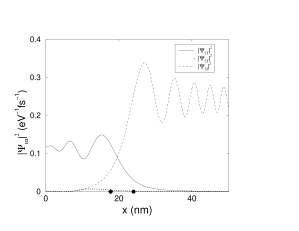
Figure 2: $|\psi_{1T}|^{2}$, $|\psi_{2T}|^{2}$ and $|\psi_{3I}|^{2}$ at $t=10$ fs versus $x$. mass=0.067$m_{e}$, $E_{q}=0.3$eV, $V_{0}=0.3$eV, $V_{0}^{\prime}=0.8$eV.

IV Examples

Figure 3: $|\psi|^{2}$ versus $x$ for $t=10$ fs (upper figure) and $t=50$ fs (lower figure). Exact solution (solid line). The diamond marks $p_{0}t/m$; the circle $p_{0}^{\prime}t/m$; the square $-q_{0}t/m$. mass=0.067$m_{e}$, $E_{q}=0.3$eV, $V_{0}=0.3$eV, $V_{0}^{\prime}=0.8$eV.

Figure 3 shows a typical wavefunction “density” versus $x$ at two fixed instants $t_{2}>t_{1}>0$ for $V_{0}^{\prime}>V_{0}>0$. For $x>0$ the main features are two flatter regions representing the old (to the right) and new (to the left) stationary regimes separated by an oscillating structure. A simple semiclassical picture provides a good zeroth order explanation: assume a stationary flux of classical particles in the old potential, with incident momentum $q_{0}$ and transmitted momentum $p_{0}$. After the potential switch at $t=0$, the last transmitted particle with momentum $p_{0}$ will be at $p_{0}t/m$, whereas the first transmitted particle with momentum $p_{0}^{\prime}$ will be at $p_{0}^{\prime}t/m$. Since $p_{0}^{\prime}>p_{0}$ there is a region of width $(p_{0}^{\prime}-p_{0})t/m$ where the two types of particles coexist. In the corresponding quantum scenario one may expect interference and oscillations of wavelenght $2\pi\hbar/(p_{0}^{\prime}-p_{0})$ in this region, whereas the regions dominated by only one plane wave the density does not oscillate and is proportional to the corresponding transmission probability, either $|T_{0}^{l}(q_{0})|^{2}$ for the “old wave” or $|T^{l}(q_{0})|^{2}$ for the “new wave”, which in the present case is smaller than the former, a somewhat surprising feature of quantum scattering off potential steps from the perspective of classical mechanics. The two crytical positions are marked in the figure with a diamond and a circle. The average local frequency Cohen95 ; MB00 shows also the transition between the two regimes, see Fig. 4.

The $x<0$ region is clearly divided into “old” (to the left) and “new” regimes where incident and reflected components interfere. They admit also a simple analysis: since the reflected wave stays dominated by momentum $-q_{0}$, the interference pattern wavelenght stays the same in the new and old regimes, $(\pi\hbar/q_{0})$, and the only difference is the amplitude change due to the change of reflection probability from $|R_{0}^{l}(q_{0})|^{2}$ to $|R^{l}(q_{0})|^{2}$. The transition at $x=-q_{0}t/m$ is marked with a square in Fig. 3.

In the example shown the dominant terms for $x>0$ are $\psi_{3T}$ and $\psi_{1I}$ representing respectively the “old” and “new” wave. Eq. (41) with these two terms only provides a very good approximation. For $x<0$ the dominant terms are $\psi_{1I}$ (incident wave), $\psi_{2I}$ (old reflected wave) and $\psi_{1R}$ (new reflected wave). Again, the analytical approximation describes the main features correctly. We may expect a worse performance of the analytical approximation in processes involving tunnelling or evanescent waves, with the pole lying close to the branch cut: for example, when $E_{q}<0$, or $-V_{0}^{\prime}>E_{q}>0$. Some of these processes and the corresponding time scales have been studied recently in GVDM02 so we shall not insist on them here.

Figure 4: $\hbar\times\omega_{av}$ versus time at $x=100$nm, where the average local frequency is defined as $\omega_{av}\equiv-{\rm Im}[(d\psi/dt)/\psi]$. Mass=0.067$m_{e}$, $E_{q}=0.3$eV, $V_{0}=0.3$eV, $V_{0}^{\prime}=0.8$eV. The diamond and circle indicate $xm/p_{0}^{\prime}$ and $xm/p_{0}$ respectively. The initial value is $V_{0}+E_{q}-V_{0}^{\prime}$ whereas the final asymptotic value is $E_{q}$.

Figure 5: $|\psi|^{2}$ versus $x$: mass=0.067$m_{e}$, $E_{q}=0.3$eV, $V_{0}=0.8$eV, $V_{0}^{\prime}=0.2$eV. The square is at $-q_{0}t/m$, the circle at $p_{0}^{\prime}t/m$ and the diamond at $p_{0}t/m$.

Fig. 5 shows the density for a case in which $V_{0}>V_{0}^{\prime}>0$. The new wave moves now at a slower pace than the old one so there is no interference structure between the two.

V Comparison with an approximate method

Figure 6: $J\times 100$ at the left box edge, $x=-22.48$nm. mass=0.042$m_{e}$, $E_{q}=0.04$eV, $V_{0}=0.42$eV, $V_{0}^{\prime}=0.62$eV; box lenght: $L=44.96$nm; number of grid points: $N=10^{4}$; time step: $\Delta t=10^{-6}$fs. The circle is at $t=xm/q_{0}$. The two stright lines indicate the values of $J\times 100$ for the initial and final stationary functions.

Figure 7: $J\times 100$ at $x=0$: exact (solid line) and for two different box lenghts: $L=179.84$nm, $N$=80000, $\Delta t=5.e-5$fs (dashed line); and $L=44.96nm$ with the same grid density and $\Delta t$ as in the other box (dots). mass=0.042$m_{e}$, $E_{q}=0.04$eV, $V_{0}=0.42$eV, $V_{0}^{\prime}=0.62$eV

Figure 8: $J\times 100$ at the right box edge, $x=22.48$nm. mass=0.042$m_{e}$, $E_{q}=0.04$eV, $V_{0}=0.42$eV, $V_{0}^{\prime}=0.62$eV; box lenght: $L=44.96$nm; number of grid points: $N=10^{4}$; time step: $\Delta t=10^{-6}$fs. The circle is at $xm/p_{0}^{\prime}$ and the diamond at $xm/p_{0}$. The two stright lines indicate the values for initial and final stationary functions.

As stated in the Introduction, the basic difficulty to deal with transient phenomena between stationary scattering states by means of grid methods is that the time dependent boundary conditions at the box edges are not known a priori. Several approximate schemes have been proposed to overcome this difficulty, and our exact solution provides a needed reference to test their validity and/or range of applicability. We have in particular made a comparison with a method proposed by Mains and Haddad MH88 based on looking a short distance into the simulation domain to determine what is coming out. Especifically, at the left edge region the wave is written as

$$\psi_{l}=Ae^{iq_{0}x/\hbar}+B(x,t)e^{-iq_{0}x/\hbar},$$ (49)

Substituting this form in the Schrödinger equation and neglecting the second order derivative of $B$,

$$i\hbar\frac{\partial\psi_{l}}{\partial t}\approx\frac{q_{0}^{2}}{2m}\psi_{l}+i\frac{\hbar q_{0}}{m}\frac{\partial B(x,t)}{\partial x}e^{-iq_{0}x/\hbar}.$$ (50)

The first derivative of $B$ is then calculated numerically at each time step with the first two spatial points, and is used to update the boundary condition for the next time step as

$$\psi(t+\Delta t)_{l}\approx\psi(t)_{l}e^{-iE_{q_{0}}\Delta t/\hbar}+\frac{q_{0}}{m}\frac{\partial B(x,t)}{\partial x}e^{-iq_{0}x/\hbar}\Delta t.$$ (51)

Similarly, the wave function at the right edge grid points is written as

$$\psi_{r}=C(x,t)e^{ip_{0}^{\prime}x/\hbar}.$$ (52)

Assuming again that $C$ is linear in $x$ and evaluating its derivative numerically with the two last grid points the boundary condition to the right is updated as

$$\psi(t+\Delta t)_{r}\approx\psi(t)_{r}e^{-iE_{q_{0}}\Delta t/\hbar}-\frac{p_{0}^{\prime}}{m}\frac{\partial C(x,t)}{\partial x}e^{-ip_{0}^{\prime}x/\hbar}\Delta t.$$ (53)

We have adapted Koonin’s grid method Koonin85 based on the Caley transform to this boundary-condition scheme and have calculated the “flux” versus time at the box edges (Figures 6 and 8) and at the center $x=0$ (Figure 7) for the same potential jump considered in MH88 ; the effective mass is taken as $m=0.042$ au (for In_0.53Ga_0.47As-AlAs) and the inicident energy corresponds to the Fermi level.

The comparison with the exact results demonstrates that the linear ansatz is quite good at the right edge but fails at the left edge, where incident and reflected components interfere. The error introduced at the left edge propagates and affects eventually to whole simulation domain, in particular the flux at the origin is deformed with respect to the exact one quite rapidly. Enlarging the box retardates the deviation from the exact result, see Fig. 7, but the computational cost becomes exceedingly large to reproduce correctly the whole transient at the origin.

VI Discussion and conclusions

Since its discovery by Tsu and Esaki, tunneling through semiconductor nanostructures has been the object of a great attention due to its possible applications to ultrahigh speed electronic devices h1 . With the development of novel semiconductor nanostructures, it has become important to carry out theoretical and experimental studies on the tunneling process of carriers when an external bias is applied. In this way, electric field-induced electron transport has been recently explored in quantum dot arrays h2 , resonant tunneling diodes h3 , and semiconductor superlattices h4 . However, we note that one remaining key question in these experiments is the analysis of the device transient response to an instantaneous potential step switching. The characteristic time of the response is of practical interest to determine the nanostructure transport properties and its possible applications to novel ultrahigh speed semiconductor devices.

We have obtained an exact solution of the transition between two stationary scattering states due to the sudden change in a potential step. Equivalently, we have solved exactly the Moshinski shutter problem for an arbitrary cut-off plane wave in the step potential. (For other potential shapes see TKF87 ; JJ89 ; Kleber94 ; BM96 ; GCV01 ). The explicit expressions obtained for their time evolution would in fact be directly applicably to an arbitrary cut-off potential with different asymptotic levels by using the appropriate transmission and reflection amplitudes. (For recent work on step-like potentials scattering see BEM01a ; BEM01b ). The exact results allow to identify characteristic times for the transients. They also provide a needed reference for testing approximate methods that model time dependent open systems (finite systems exchanging particles with the outside) with injecting and absorbing boundary conditions.

Appendix A Reflection and transmission amplitudes

The reflection and transmission amplitudes in stationary waves with left and right incidence are given by

$$\begin{array}[]{ll}R^{l}(q)=\frac{q-p}{q+p},&T^{l}(q)=\frac{2q}{q+p}\\ R^{r}(p)=\frac{p-q}{q+p},&T^{r}(p)=\frac{2p}{q+p}\end{array}$$ (54)

for positive values of the arguments. The analytical continuations for negative arguments are the amplitudes for the “outgoing” or “time-reversed” stationary states.

Appendix B Wave functions

These are the time dependent wave functions corresponding to the initial conditions given in Eqs. (6-9) for the potential of Eq. (5):

$$\psi_{1,2}=\frac{i}{2\pi\sqrt{h}}\left\{\begin{array}[]{l}\int_{C_{j}}dq\,\frac{e^{-iE_{q}t/\hbar}}{q\mp q_{0}+i0}(e^{iqx/\hbar}+\frac{q-p}{q+p}e^{-iqx/\hbar}),\;x\leq 0\\ \int_{C_{j}}dp\,\frac{2pe^{ipx/\hbar}e^{-iE_{q}t/\hbar}}{(q+p)(q\mp q_{0}+i0)},\;x\geq 0\end{array}\right.$$ (55)

where the minus and plus signs correspond to $\psi_{1}$ and $\psi_{2}$ respectively, and

$$\psi_{3,4}=\frac{-i}{2\pi\sqrt{h}}\left\{\begin{array}[]{l}\int_{C_{j}}dq\,\frac{2qe^{iqx/\hbar}e^{-iE_{q}t/\hbar}}{(q+p)(p\mp p_{0}-i0)},\;x\leq 0\\ \int_{C_{j}}dp\,\frac{e^{-iE_{q}t/\hbar}}{p\mp p_{0}-i0}(e^{ipx/\hbar}+\frac{p-q}{q+p}e^{-ipx/\hbar}),\;x\geq 0\end{array}\right.$$ (56)

with the minus sign for $\psi_{3}$ and the plus sign for $\psi_{4}$.

Term	support	-b/2a	pole	H-term	$e^{iV_{0}^{\prime}t/\hbar}$	contour	$A_{0}$	$k_{0}$	$g$
$\psi_{1T}$	$x>0$	$xm/t>0$	$q_{0}-i0$	yes	yes	above	$T^{l}(q_{0}-i0)$	$p(q_{0}-i0)$	$\frac{p}{q}\frac{T^{l}(p)}{q-q_{0}+i0}$
$\psi_{1I}$	$x<0$	$xm/t<0$	$q_{0}-i0$	no	no	above	$1$	$q_{0}-i0$	$\frac{1}{q-q_{0}+i0}$
$\psi_{1R}$	$x<0$	$-xm/t>0$	$q_{0}-i0$	yes	no	above	$R^{l}(q_{0}-i0)$	$q_{0}-i0$	$\frac{R^{l}(q)}{q-q_{0}+i0}$
$\psi_{2T}$	$x>0$	$xm/t>0$	$-q_{0}-i0$	yes	yes	above	$T^{l}(-q_{0}-i0)$	$p(-q_{0}-i0)$	$\frac{p}{q}\frac{T^{l}(p)}{q+q_{0}+i0}$
$\psi_{2I}$	$x<0$	$xm/t<0$	$-q_{0}-i0$	no	no	above	$1$	$-q_{0}-i0$	$\frac{1}{q+q_{0}+i0}$
$\psi_{2R}$	$x<0$	$-xm/t>0$	$-q_{0}-i0$	yes	no	above	$R^{l}(-q_{0}-i0)$	$-q_{0}-i0$	$\frac{R^{l}(q)}{q+q_{0}+i0}$
$\psi_{3I}$	$x>0$	$xm/t>0$	$p_{0}+i0$	no	yes	below	$1$	$p_{0}+i0$	$\frac{1}{p-p_{0}-i0}$
$\psi_{3R}$	$x>0$	$-xm/t<0$	$p_{0}+i0$	yes	yes	below	$R^{r}(-p_{0}-i0)$	$p_{0}+i0$	$\frac{R^{r}(-p)}{p-p_{0}-i0}$
$\psi_{3T}$	$x<0$	$xm/t<0$	$p_{0}+i0$	yes	no	below	$T^{r}(-p_{0}-i0)$	$q(p_{0}+i0)$	$\frac{q}{p}\frac{T^{r}(-p)}{p-p_{0}-i0}$
$\psi_{4I}$	$x>0$	$xm/t>0$	$-p_{0}+i0$	no	yes	below	$1$	$-p_{0}+i0$	$\frac{1}{p+p_{0}-i0}$
$\psi_{4R}$	$x>0$	$-xm/t<0$	$-p_{0}+i0$	yes	yes	below	$R^{r}(p_{0}-i0)$	$-p_{0}+i0$	$\frac{R^{r}(-p)}{p-p_{0}-i0}$
$\psi_{4T}$	$x<0$	$xm/t<0$	$-p_{0}+i0$	yes	no	below	$T^{r}(p_{0}-i0)$	$q(-p_{0}+i0)$	$\frac{q}{p}\frac{T^{r}(-p)}{p-p_{0}-i0}$

Table 1: Features of the terms $\psi_{j\alpha}$.

References

• (1) R. K. Mains and G. I. Haddad, J. Appl. Phys. 64, 3564 (1988).
• (2) W. R. Frensley, Rev. Mod. Phys. 62, 745 (1990).
• (3) K. Register, U. Ravaioli, K. Hess, J. Appl. Phys. 69 7153 (1991); 1555 (E) (1992).
• (4) M. C. Yalabik and M. I. Ecemis, Phys. Rev. B 51, 2082 (1995).
• (5) C. L. Hammer, T. A. Weber, and V. S. Zidell, Am. J. Phys. 45, 933 (1977).
• (6) M. Moshinsky, Phys. Rev. 88, 625 (1952).
• (7) J. G. Muga and C. R. Leavens, Phys. Rep. 338, 353 (2000).
• (8) J. G. Muga, R. Sala and I. L. Egusquiza (eds.), Time in Quantum Mechanics (Springer, Berlin, 2002).
• (9) H. M. Nussenzveig in Symmetries in Physics, ed. by A. Frank and F. B. Wolf (Springer-Verlag, Berlin 1992), Chap. 19
• (10) L. Cohen, Time-Frequency analysis (Prentice Hall, New Jersey, 1995).
• (11) J. G. Muga and M. Büttiker, Phys. Rev. A 62, 023808 (2000).
• (12) G. García-Calderón, J. Villavicencio, F. Delgado and J. G. Muga, quant-ph/0206020, to appear in Phys. Rev. A.
• (13) S. E. Koonin, Computational Physics (Benjamin, Menlo Park, NJ, 1985).
• (14) N. Teranishi, A. M. Kriman and D. K. Ferry, Superlatt. Microstruct. 3, 509 (1987).
• (15) A. P. Jauho and M. Jonson, Superlatt. Microstruct. 6, 303 (1989).
• (16) M. Kleber, Phys. Rep. 6, 331 (1994).
• (17) S. Brouard and J. G. Muga, Phys. Rev. A 96, 3055 (1996).
• (18) G. García Calderón and J. Villavicencio, Phys. Rev. 64, 012107 (2001).
• (19) A. D. Baute, I. L. Egusquiza and J. G. Muga, J. Phys. A 34, 4289 (2001).
• (20) A. D. Baute, I. L. Egusquiza and J. G. Muga, J. Phys. A 34, 5341 (2001).
• (21) R. Tsu and L. Esaki, Appl. Phys. Lett. 22, 562 (1973); L. Esaki, IEEE J. Quantum Electron. 22, 1611 (1986).
• (22) J. P. Bird, R. Akis, D. K. Ferry, D. Vasikska, J. Cooper, Y. Aoyagi and T. Sugano, Phys. Rev. Lett. 82, 4691 (1999).
• (23) T. M. Fromhold, P. B. Wilkinson, F. W. Sheard, L. Eaves, J. Miao and G. Edwards, Phys. Rev. Lett. 75, 1142 (1995).
• (24) P. Pereyra, Phys. Rev. Lett. 80, 2677 (1998).