On resumming periodic orbits in the spectra of integrable systems

Abstract

Spectral determinants have proven to be valuable tools for resumming the periodic orbits in the Gutzwiller trace formula of chaotic systems. We investigate these tools in the context of integrable systems to which these techniques have not been previously applied. Our specific model is a stroboscopic map of an integrable Hamiltonian system with quadratic action dependence, for which each stage of the semiclassical approximation can be controlled. It is found that large errors occur in the semiclassical traces due to edge corrections which may be neglected if the eigenvalues are obtained by Fourier transformation over the long time dynamics. However, these errors cause serious harm to the spectral approximations of an integrable system obtained via the spectral determinants. The symmetry property of the spectral determinant does not generally alleviate the error, since it sometimes sheds a pair of eigenvalues from the unit circle. By taking into account the leading order asymptotics of the edge corrections, the spectral determinant method makes a significant recovery.

I Introduction

It has been generally accepted that spectral determinants, or zeta-functions, provide optimal semiclassical estimates of the individual energy levels of classically chaotic systems cv ; Cvitanovic89 ; Eckhardt89 . These resummations of the periodic orbits in the Gutzwiller trace formula Gutzwiller71 ; Balian72 , originally developed for time-independent systems, may be obtained in a variety of ways. The formulation of Berry and Keating Berry90JPA relies explicitly on the instability of the periodic orbits in such a way as to give an expression that does not depend on a sharp cut-off of the orbit periods. In contrast, Bogomolny’s approach Bogomolny90 ; Bogomolny92 reduces the problem to the quantization of a map over a Poincareé surface of section, without making any assumption about the nature of the classical motion. However, two sharp boundaries are introduced. On the one hand, the Poincareé section itself is bounded if the constant energy surface is compact. The limited area of the section, which corresponds to a finite dimension of the Hilbert space, then leads to a sharp cut-off in the period of the orbits. The recent paper of Eckhart and Smilansky Eckhardt01 also works with a quantum map in a bounded region, but this is obtained stroboscopically instead of with a Poincaré section.

The classical motion of integrable systems is restricted to invariant tori, which determine closed invariant curves (also tori) of the Poincaré mapping. For integrable systems, Berry and Tabor bt established the equivalence of the Gutzwiller trace formula to the general forms of Bohr-Sommerfeld quantization. The latter method is evidently the most efficient for the calculation of individual levels. Nevertheless the exercise of showing the equivalence of both methods had the merit of clarifying the role of periodic orbits (forming continuous tori for higher dimensional systems) in the density of states. Indeed it raises an important question: The Berry-Tabor equivalence involves the complete set of periodic orbits, so how might one obtain correct energy levels from the resummation of a finite selection of short orbits?

Our interest in this paper is resummation approximations for the spectra of simple integrable systems. Particularly, we will focus on the effect of introducing boundaries that do not interfere with the local classical tori. For simplicity, consider such a system with a single degree of freedom. For the classical Hamiltonian $H(I)$, where $(I,\theta)$ are the action-angle variables text , the Bohr-Sommerfeld levels are

$$E_{n}=H\left(\hbar\left(n+{1\over 2}\right)\right)\ .$$ (1)

Actually, it suffices to consider a case for which the action variables are those of the harmonic oscillator

$$I={1\over 2}(p^{2}+q^{2})\ ,$$ (2)

rendering the semiclassical approximation of  (1) exact. It is important to point out that large-$n$ states are well approximated by  (1) even for a general nonquadratic dependence of the Hamiltonian on the phase space variables. The main question is how well a spectral determinant method converges to the eigenvalues $E_{n}$ in this case.

A conceptually clean approach to answering this question follows in the spirit of Creagh Creagh95 , who applied an extension of resummation methods Saracero92 ; Smilansky93JPA to the perturbed cat maps. He found worsening errors in the semiclassical trace formula as the perturbation brought the map out of the hyperbolic regime, but was unable to continue the perturbation all the way to an integrable regime. Here, since $I$ is a constant of the classical evolution, our consideration can be limited to a ring ${\cal I}_{-}<I<{\cal I}_{+}$, thus obtaining a finite phase space and hence a finite Hilbert space of dimension $N=\{({\cal I}_{+}-{\cal I}_{-})/\hbar\}$, where $\{\ \cdot\ \}$ denotes the integer part. A stroboscopic map of period $\tau$ can be defined and quantized in such a way that the dynamics is determined by the evolution operator

$$U_{N}=\sum_{n=N_{-}}^{N_{+}}\exp\!\left(-{i\over\hbar}E_{n}\tau\right)|n\rangle\langle n|\ .$$ (3)

The quantity $\hbar N_{-}$ ($\hbar N_{+}$) is the smallest (largest) quantized action greater (smaller) than ${\cal I}_{-}$ (${\cal I}_{+}$) and $|n\rangle$ are the eigenstates. The definition of the spectral determinant as $\det\left(1-zU_{N}\right)$ gives an $N^{th}$ order polynomial in the variable $z$ and the roots of the characteristic equation

$$P_{N}(z)\equiv\det\left(1-zU_{N}\right)=0$$ (4)

are just

$$z_{n}=\exp\left({i\over\hbar}E_{n}\tau\right)\ .$$ (5)

Thus, knowledge of the phases $\phi_{n}$ of the zeros of the spectral determinant, or zeta-function, determines the eigenvalues of the stroboscopic map within the ring. These coincide with a subset of the eigenvalues of the original system possessing an infinite Hilbert space.

The eigenenergies of the original system can be inferred from

$$E_{n}={\hbar\over\tau}(\phi_{n}+2k\pi)\ .$$ (6)

The determination is unique if, for the energy interval of the ring $(E_{-},E_{+})=(E({\cal I}_{-}),E({\cal I}_{+}))$, the constraint

$$\left(E_{+}-E_{-}\right){\tau\over\hbar}\leq 2\pi$$ (7)

is respected. This scheme for locating eigenvalues of the original Hamiltonian resembles that of Eckhardt01 , but our objective of comparing semiclassical methods can be achieved also in the context of the continuous dynamical system confined to the ring, or even the discrete map defined by (3).

In the semiclassical limit, $\mbox{Tr}(U_{N}^{l})$ is expressed as a sum over periodic orbits of period $l$ for the classical stroboscopic map generated by the Hamiltonian $H(I)$ in the time $\tau$ within the ring. These orbits, with action $I_{m,l}$, such that

$$\tau{{\rm d}H(I)\over{\rm d}I}={2\pi m\over l}\ ,$$ (8)

define continuous curves, unless $I=0$. To simplify the treatment, we consider ${\cal I}_{-}>0$, which excludes the isolated periodic orbit at the origin.

Note that the periodic orbits of the stroboscopic map comprise only a small subset of those of the original system with continuous time. Indeed, all the orbits of the latter are periodic whereas only those full orbits with periods that are rationally related to the stroboscopic time, $\tau$, are periodic in the map. The map resembles a Poincaré map of an integrable system with two degrees of freedom in the sense that all orbits lie on invariant curves, but the curves made up of periodic orbits form a dense set of zero measure.

The semiclassical form for the spectral determinant is obtained from the expression

$$\det\left(1-zU_{N}\right)=\exp\left[-\sum_{l=1}^{\infty}{z^{l}\over l}\ \mbox{Tr}(U_{N}^{l})\right]\ .$$ (9)

Even though the series only converges for $|z|<1$, it is possible to follow Saracero92 in noting that the Taylor expansion of the exponential in Eq. (9) can be identified with the finite expansion of the spectral determinant (4):

$$P_{N}(z)=1+c_{1}z+c_{2}z^{2}...+c_{N}z^{N}\ ,$$ (10)

where the coefficients are given by the following recurrence relation

$$c_{k}=-\frac{1}{k}\sum_{l=1}^{k}c_{k-l}\mbox{Tr}\,(U_{N}^{l})\ .$$ (11)

In this way the periodic orbits up to period $l=N$ determine, in principle, all the eigenvalues of $U_{N}$.

A further reduction of the period of the orbits used in the semiclassical spectral determinant results from the symmetry relation for the coefficients Bogomolny90

$$c_{k}=(-1)^{N}\det(U_{N})c_{N-k}\ .$$ (12)

The coefficients containing traces for long iteration times, $l>N/2$, can be obtained from the coefficients with $l<N/2$. Hence, only the orbits of period $l<N/2$ are needed. This is a particularly simple example of “bootstrapping” Berry85 resulting from the finiteness of the Hilbert space. For chaotic systems, the symmetry (12) is a fundamental tool because the number of periodic orbits increases exponentially with $l$. This is not so for integrable systems.

In Section II, we derive the semiclassical formula for $\mbox{Tr}(U^{l})$ of the integrable map defined in  (3). It will then become clear that edge corrections to the periodic orbit sum cannot be neglected in this case. Indeed these are the only corrections for the particular model that we study numerically in Section IV. Though the absence of edge corrections severely affects the spectral determinant, which has a natural cut-off in time, they cancel out in the Berry-Tabor formula as discussed in Section III.

II The semiclassical trace

Relation (1) for the eigenvalues becomes exact in the case of the harmonic oscillator actions (2). Likewise, the propagator (3), extended to all $n$, would give the full evolution operator for any given function of the projection operators $|n\rangle\langle n|$. However, the initial semiclassical approximation is to consider the action-angle variables $(I,\theta)$ as appropriate conjugate variables for quantization. From the action representation of the operator $U_{N}^{l}$, the $l^{th}$ power of $U_{N}$ in  (3), the matrix elements in the angle representation turn out to be

$$\langle\theta|U_{N}^{l}|\theta^{\prime}\rangle={1\over 2\pi}\sum_{n=N_{-}}^{N_{+}}\exp\left\{i\left[\left(n+{1\over 2}\right)(\theta-\theta^{\prime})-l{\tau E_{n}\over\hbar}\right]\right\}\ ,$$ (13)

where we used $\langle\theta|n\rangle=e^{-i\left(n+{1\over 2}\right)\theta}/\sqrt{2\pi}$.

The Poisson transformation is now applied, changing to the continuous action variable $I$, so that $E$ is interpolated by $H(I)$ as in  (1). This results in

$$\langle\theta|U_{N}^{l}|\theta^{\prime}\rangle={1\over 2\pi\hbar}\sum_{m={-\infty}}^{\infty}(-1)^{m}\int_{{\cal I}_{-}}^{{\cal I}_{+}}{\rm d}I\exp\left\{{i\over\hbar}\Big{[}I(\theta-\theta^{\prime})+2\pi m-l\tau H(I)\Big{]}\right\}\ ,$$ (14)

which is exactly equivalent to (13). Tracing over the angle variables gives

$$\mbox{Tr}(U_{N}^{l})={1\over\hbar}\sum_{m={-\infty}}^{\infty}(-1)^{m}\int_{{\cal I}_{-}}^{{\cal I}_{+}}{\rm d}I\exp\left\{{i\over\hbar}\Big{[}2\pi mI-l\tau H(I)\Big{]}\right\}\ .$$ (15)

The exponential in the integrand of (15) oscillates rapidly in the semiclassical limit, and the largest contributions to the trace, of order $\hbar^{1/2}$, come from the regions near the stationary phase points at

$$l\tau{{\rm d}H(I)\over{\rm d}I}-2\pi m=0\ ,$$ (16)

which is the same condition as the one given by (8) for the periodic orbits of the classical stroboscopic map. The stationary phase evaluation of the trace is therefore tied to the periodic orbits with actions $I_{m,l}$.

The periodic orbits can now be ordered by increasing period, $l$. Equation (16) also sets the range of possible repetitions $(M_{l-},M_{l+})$ of the period $l$ orbit. The frequencies, $\omega={{\rm d}H(I)/{\rm d}I}$ in the limited range of action $({\cal I}_{-},{\cal I}_{+})$ are also bounded. Thus, the number of periodic orbits in this range increases linearly with $l$. The full stationary phase evaluation of (15) becomes

$$\mbox{Tr}(U_{N}^{l})=\sum_{m=M_{l-}}^{M_{l+}}(-1)^{m}\left({2\pi\over\hbar l\tau\left|{{\rm d^{2}}H(I)\over{\rm d}I^{2}}\right|_{I_{m,l}}}\right)^{1/2}\!\!\!\exp\left\{{i\over\hbar}\left[2\pi mI_{m,l}-l\tau H(I_{m,l})-\hbar{\pi\over 4}\right]\right\}\ .$$ (17)

Not only are the stationary points of the integration specified by the action variables of the periodic orbits, but the phase of each contribution is given by the full action in units of $\hbar$,

$${\cal S}_{m,l}=\int_{0}^{l\tau}{\rm d}t\ \left[p\dot{q}-H\right],$$ (18)

except for the geometric “Maslov term”, $\pi/4$.

Typically, the contributions to the trace from the endpoints ${\cal I}_{\pm}$ to the integrals in (15) are only of order $\hbar$. However, note that they cannot be separated from the stationary phase term corresponding to a periodic orbit which lies very close to the boundary. In fact, by varying the parameters of the system and $l$, essentially all the stationary phase points pass close to the boundaries. The edge corrections can be obtained as a uniform approximation Eckhardt01 , but this erases the simplicity of the periodic orbit expression for the trace. It is shown in the following section that the limitation of the allowed phase space to the ring $({\cal I}_{-},{\cal I}_{+})$ in no way hinders the Berry-Tabor equivalence.

III The Berry-Tabor equivalence

A version of the Gutzwiller trace formula that is appropriate to an integrable map is simply obtained by Fourier analyzing the traces of $U_{N}^{l}$ in the discrete time $l$:

$$\sum_{l=0}^{\infty}e^{il\theta}\mbox{Tr}(U_{N}^{l})=\mbox{Tr}{1\over 1-e^{i\theta}U_{N}}=\sum_{n}{1\over 1-\exp[i(\theta-l\tau E_{n})]}\ .$$ (19)

Here, the eigenvalues of the map are considered as poles of the resolvent $(1-zU_{N})^{-1}$ instead of zeros of $\det(1-zU_{N})$.

Though the infinite series of traces in (19) appears to be a cumbersome alternative to evaluating the finite determinant, Poisson transformation to the periodic orbit expression can be performed for the semiclassical resolvent,

$$\mbox{Tr}{1\over 1-e^{i\theta}U_{N}} = \sum_{m,l}(-1)^{m}\left({2\pi\over\hbar l\tau\left|{{\rm d^{2}}H(I)\over{\rm d}I^{2}}\right|_{I_{m,l}}}\right)^{1/2}$$ (20)

$$\times\exp\left({i\over\hbar}\left[\hbar l\theta+2\pi mI_{m,l}-l\tau H(I_{m,l})-\hbar{\pi\over 4}\right]\right)\ .$$

Interpolating the discrete time $l$ again by the continuous time $s$ gives

$$\mbox{Tr}{1\over 1-e^{i\theta}U_{N}} = \sum_{k}(-1)^{m}\left({2\pi\over\hbar\tau l\left|{{\rm d^{2}}H(I)\over{\rm d}I^{2}}\right|_{I_{m,s}}}\right)^{1/2}$$ (21)

$$\times\int_{0}^{\infty}{\rm d}s\ \exp\left\{{i\over\hbar}\left[\hbar s\theta+2\pi(mI_{m,s}+\hbar ks)-s\tau H(I_{m,s})-\hbar{\pi\over 4}\right]\right\}\ .$$

The stationary phase points, $s_{m,k}(\theta)$, of the integrals in Eq. (21) are given by

$${{\rm d}{\cal S}_{m,s}\over{\rm d}s}+\hbar(\theta+2\pi k)=0$$ (22)

where ${\cal S}_{m,s}$ is the full action of the orbit singled out by condition (16). It is important to note that, while in (16), the stationary phase condition defined a periodic orbit of integer period $l$ for the $\tau$-stroboscopic map, now $l$ has been replaced by the continuous variable $s$. This condition can be reinterpreted in two ways: (i) orbits are picked that are no longer closed, or (ii) the selected orbit is still periodic, but for a different $\tau(\theta)$. In either case,

$${{\rm d}{\cal S}_{m,s}\over{\rm d}s}=\tau{{\rm d}{\cal S}_{m,s}\over{\rm d}t}=\tau E_{m,s}\ ,$$ (23)

where the energy of the selected orbit appears in the last equality. Thus, the resulting phase of each integral is given by the reduced action for the orbits of energy $\hbar(\theta+2\pi k)/\tau$. The stationary evaluation of the resolvent is

$$\mbox{Tr}{1\over 1-e^{i\theta}U_{N}}\approx\sum_{k,m}s_{1,k}(\theta)\>\exp\left[{i\over\hbar}2\pi mI\left({\hbar\over\tau}(\theta+2\pi k)\right)+i\pi m\right]\ ,$$ (24)

where $I(E)$ is the local inverse of $H(I)$. Thus, if $\hbar/\tau$ is chosen such that the variation of $\tau H(I)/\hbar$ does not exceed $2\pi$ for $I$ in $({\cal I}_{-},{\cal I}_{+})$, there are at most a few orbits contributing to the semiclassical resolvent for each value of $\theta$. Since the repetitions must still be summed, the interpretation (ii) for (22) as a periodic orbit of another stroboscopic map is perhaps the more appealing.

The condition for the resolvent to be singular is that all the $m$ repetitions are exactly in phase,

$$I\!\left({\hbar\over\tau}(\theta+2\pi k)\right)=\left(j-{1\over 2}\right)\pi\ ,$$ (25)

which is just the initial Bohr-Sommerfeld quantization. Thus, the periodic orbit evaluation of the map resolvent retrieves the full Berry-Tabor equivalence without any need to consider boundary corrections to the trace. The reason why this works is that the singularities of the resolvent only manifest themselves by summing the periodic contributions for very long times, or multiple repetitions. For these contributions there is an effective increase of the large parameter of the stationary phase evaluation of $\mbox{Tr}(U_{N}^{l})$ given by (17). The integrals are then dominated by a very narrow region near each periodic orbit, so that the boundary can be ignored for the high repetition of an orbit even if it lies almost at the edge.

The evaluation of the spectral determinant may be regarded as a resummation of the semiclassical sum for the poles of the resolvent, such that the (discrete) time of the contributing periodic orbits is cut-off by the dimension of the finite Hilbert space. We show in the next section that the error in the traces of the propagator due to the edge corrections can be magnified by the spectral determinant.

IV Model Hamiltonian

To illustrate the calculation of the spectral determinant, we choose the simplest Hamiltonian that is a nonlinear function of the action, namely

$$H(I)={1\over 2}(I-{\cal I})^{2}\qquad(I\geq 0)\ .$$ (26)

The periodic orbit condition (8) then reduces to

$$I_{m,l}={\cal I}+2\pi{m\over l\tau}\$$ (27)

and the stationary phase evaluation of the trace assumes the explicit form

$$\mbox{Tr}(U_{N}^{l})\approx\left({2\pi\over\hbar l\tau}\right)^{1/2}e^{-i\pi/4}\sum_{m}(-1)^{m}\exp\left[{i\over\hbar}2\pi m\left({\cal I}+{\pi m\over l\tau}\right)\right]\ .$$ (28)

For the case where the parameter ${\cal I}=\hbar(n+1/2)$ (i.e. one of the quantized actions), $\mbox{Tr}(U_{N}^{l})$ reduces to a “curlicue”. These recursively spiraling patterns in the complex plane were shown by Berry and Goldberg Berry88 to have quite diverse characteristics depending on $\tau/\hbar$, in the limit $N\rightarrow\infty$. This may also be the case for non-quantized ${\cal I}$.

Two essentially different regions of the eigenspectrum can be studied. In case (i), ${\cal I}>0$ and ${\cal I}_{\pm}={\cal I}\pm\sqrt{2\cal E}<2{\cal I}$. The energy levels there originate on two different branches of $H(I)$, so there may be near degeneracies. This is a similar situation to that expected for an integrable system with more degrees of freedom (see e.g. text ). Otherwise, in case (ii), both ${\cal I}_{+}$ and ${\cal I}_{-}$ $>$ $2{\cal I}$, so that a single branch of the $H(I)$ curve is sampled. The energy levels are then quite regularly spaced with approximate separation of Planck’s constant times the average ${\rm d}H/{\rm d}I$ for this energy interval. By choosing $E_{\pm}$ to satisfy condition (7), we also guarantee the regularity of the spectrum of $U_{N}$ itself.

IV.1 Case (i)

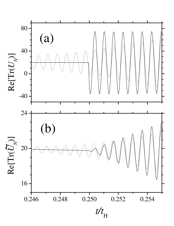
Figure 1: Comparison between the exact (dotted lines) and the semiclassical values (solid lines) of Re[Tr($U_{N})$] as a function of $t/t_{\mbox{\scriptsize H}}$ for (a) unweighted and (b) cosine weighted trace. The behaviour is similar for Im[Tr($U_{N})$] and therefore not shown here.

Let us first examine the semiclassical approximations to $\mbox{Tr}(U_{N})$ for a single period. Notice that the stationary phase approximation to the integrals in (15) would be exact for the quadratic model if the limits could be extended to $\pm\infty$. In other words, the edge corrections are the only deviation of the periodic orbit approximation with respect to the exact trace. These corrections are certainly not negligible for stroboscopic parameters such that a periodic orbit is close to one of the edges. The simplest asymptotic edge corrections, as deduced in Eckhardt01 , are presented in A. The computed error due to the edges is displayed in Figure 1. Here we let the time $t$ vary and study Tr($U_{N}$) as a function of $t/t_{\mbox{\scriptsize H}}$, where $t_{\mbox{\scriptsize H}}=2\pi\Delta N/E$ is the Heisenberg time. As the time is increased the integrand at the l.h.s. of Equation (15) has more stationary phase points. The sudden jump in the semiclassical trace in Figure 1a is due to the following. For small values of $t/t_{\mbox{\scriptsize H}}$ there is just a single stationary phase point with $m=0$. Going beyond $t/t_{\mbox{\scriptsize H}}\approx 0.25$ all $|m|\leq 1$ become stationary phase points. (It is near such transition points that the semiclassical approximation is worse.) This situation repeats itself regularly with increasing $t/t_{\mbox{\scriptsize H}}$ adding more stationary points to the sum (28). As seen in Figure 1a, the semiclassical trace as given by (28) is not an accurate approximation to the exact Tr$(U_{N})$. The suppression of the edge correction by means of a cosine weighted trace, namely

$$\mbox{Tr}(\widetilde{U_{N}})=\mbox{Tr}\left[U_{N}\cos\left(\frac{\pi H(I)}{2E}\right)\right],$$ (29)

improves the agreement enormously, as shown in Figure 1b. Our calculations have been performed for case $\hbar=0.01,E=30.4571694,$ and ${\cal I}=20.3489573$ giving $N=1~{}521$.

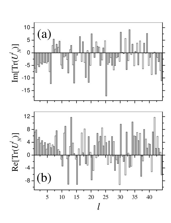
Figure 2: Comparison between the exact (white histograms) and the semiclassical (grey histograms) values of (a) Im[Tr$(U_{N}^{l}$)] and (b) Re[Tr$(U_{N}^{l}$)] as a function of $l$ for $N=48$.

We now return to the original programme of obtaining the eigenvalues of $U_{N}$, defined for a fixed $\tau$, by resumming periodic orbits. The first step is to calculate the traces of $U_{N}^{l}$. The coefficient of the characteristic polynomial are then easily computed by (11). The roots of the resulting polynomial are obtained numerically. The precision in finding the roots, limits this method to polynomials with $N\leq 50$. We chose the model Hamiltonian parameters accordingly.

To illustrate case (i), we take the parameters $E$ and ${\cal I}$ to be the same as above and $\hbar=0.35$, which gives $N=48$. Figure 2 displays the real and imaginary parts of $\mbox{Tr}(U_{N}^{l})$ for $l\leq N$ using the semiclassical expression (28) contrasted with their exact values. As expected, the semiclassical approximation works reasonably well for the lowest values of $l$ and gives very poor results for the largest ones. It is worth noticing that similar calculations with the addition of an imaginary part to the time in the trace (17) show a dramatic improvement in the agreement between the semiclassical and the exact traces. This is further evidence that the differences are due to edge corrections and not to numerical inaccuracies.

Next, we calculate the coefficients $c_{k}$ of the characteristic polynomial (4) using the recursion relation (11). The symmetry relation (12) allows us to use only traces corresponding to times shorter than $\tau_{\mbox{\scriptsize H}}/2$. In Figure 3 we compare the exact coefficients $c_{k}$ with those resulting from the semiclassical traces, with and without symmetrization. To better illustrate the whole range of $c_{k}$ we show a situation where $N=28$, corresponding to $\hbar=1.0,E=100.1234,$ and ${\cal I}=41.2345$. As before, the semiclassical approximation works well for the low $k$ coefficients ($k<5$) and, obviously, also for the corresponding higher $k$’s if we impose the symmetry (12). For the remaining coefficients, the agreement with the exact $c_{k}$ is poor.

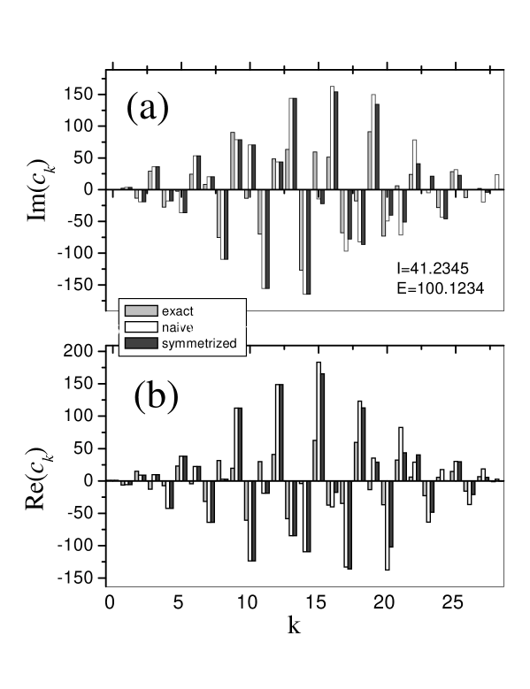
Figure 3: Comparison between the exact (gray), the semiclassical (white) and the symmetrized semiclassical (black) values of (a) Im($c_{k}$) and (b) Re($c_{k}$) as a function of $k$ for $N=28$.

Finally we arrive at the eigenvalues of $U_{N}^{l}$. Figure 4 shows the results for $\hbar=0.35,E=30.4571694,$ and ${\cal I}=20.3489573$, which is a rather typical situation. The exact roots of the characteristic polynomial lie on the unit circle, as they should. The standard semiclassical approximation destroys unitarity and the roots of the corresponding characteristic polynomial are no longer restricted to the unit circle. The enforcement of the symmetry (12) makes $|\det(U)|=1$. As a consequence the roots either lie exactly on the unit circle, or appear in pairs, one inside and one outside the circle. More precisely, the self-inversive symmetry of the characteristic polynomial renders a symmetry in its zeros: if $z_{k}$ is a root then $1/z^{*}_{k}$ is also a root. Indeed, it has been shown by Bogomolny et al.BBL96 that on average only about $57\%$ of the roots of a random symmetrical polynomial lie on the unit circle. Unfortunately, upon symmetrization individual roots do not necessarily come closer to the exact ones, as compared with the standard procedure. Figure 4 shows that they can even be pushed out, unless the standard semiclassical roots are already close to the exact ones, in which case symmetrization tends to improve the accuracy. Unfortunately this behaviour is not very systematic.

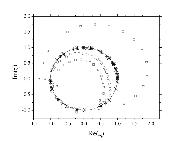
Figure 4: Comparison between the exact (asterisks), the semiclassical (open circles) and the symmetrized semiclassical (open squares) roots $z_{i}$ of the characteristic polynomial for $N=48$.

IV.2 Case (ii)

We switch now to case (ii) and consider the situation where the energy $E>{\cal I}^{2}/2$, or equivalently, both ${\cal I}_{+}$ and ${\cal I}_{-}>2{\cal I}$. As mentioned before, in this situation the levels are almost equally spaced with separation of $\hbar{\rm d}H/{\rm d}I$. From the semiclassical point of view, the most important distinction to case (i) is the absence of the $m=0$ orbit. Actually, for our simple model there will be no tori with orbits of period $l<N/2$ in case (ii). Indeed, the fraction, $f$, of zero traces in the semiclassical approximation is easily seen to be:

$$f=\frac{1}{2}\frac{\sqrt{E_{+}}+\sqrt{E_{-}}}{\sqrt{E_{+}}-\sqrt{E_{-}}}.$$ (30)

The optimum of $f\approx N/2$ is approached for $E_{-}\approx 0$, which implies ${\cal I}\leq 0$, so we choose $\hbar=1.0,{\cal I}=-1.03489573$ with $E_{-}=0.265678$ and $E_{+}=1250.0$, which corresponds to $N=48$. Keeping $\tau$ as defined by (7) gives Tr$(U_{N}^{l})=0$ for $l\leq 24$. The results are summarized by Figure 5.

As in case (i) the simple semiclassical approximation shows roots outside the unit circle. The standard semiclassical improvement by symmetrization (“bottom up symmetrization”) erases all system information, since there are only nonzero traces for long times. Indeed, the spectral determinant (10) reduces to

$$P_{N}(z)=1+(-1)^{N}\det(U_{N})\>z_{N}.$$ (31)

Instead, one can maximize the semiclassical information by symmetrizing the lower coefficients in $P_{N}(z)$ from the higher $c_{k}$’s , containing the traces with long orbits (“top down symmetrization”). However, the final result is no better than the one without symmetrizing at all.

By shifting the parameters in case (ii) so that $H(I)$ becomes almost linear, within the interval $({\cal I}_{-},{\cal I}_{+})$, the agreement between the different approaches becomes much more reasonable than in Figure 5. However, if one recalls that the mean level spacing is known and the levels are almost equally spaced, some caution is then required. The exact traces lead to a characteristic polynomial with self-inversive symmetry. For small values of $l$, where there is no stationary phase and the semiclassical traces are zero, the (modulus of) exact traces are small compared to unit. On the other hand, we observe that, for large $l$ values, the semiclassical approximation fails to reproduce the exact traces with the same precision. Thus, the best semiclassical agreement corresponds surprisingly to the case where all traces are taken as zero (bottom up). As shown in Fig 5, the top down symmetrization is superior to the standard procedure only where the eigenvalues are sufficiently accurate. It then brings most of the roots back to the unit circle. However, since it employs some inaccurate large $l$ traces, (top down) symmetrization also produces pairs of roots lying at opposite sides of the unit circle, like in case (i).

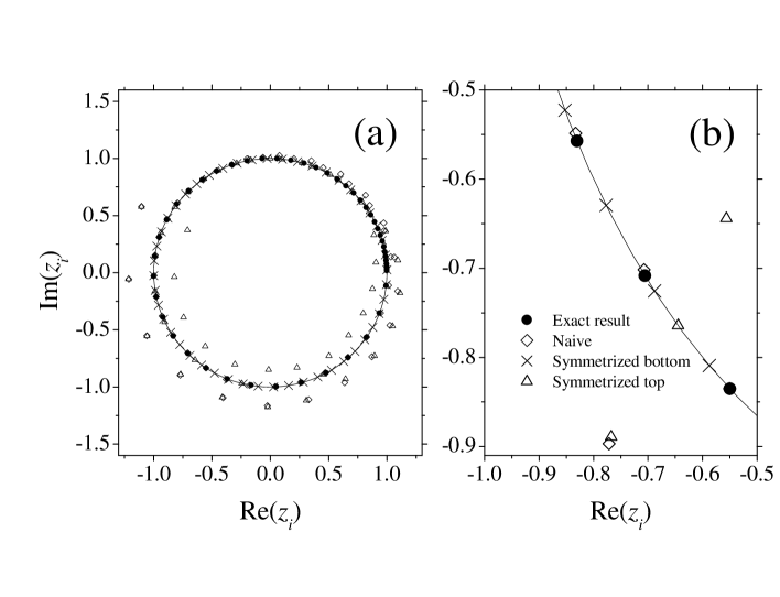
Figure 5: Comparison between the exact (crosses), the semiclassical (open circles), the “bottom” symmetrized semiclassical (open squares) and the “top” symmetrized semiclassical (open triangles) roots $z_{i}$ of the characteristic polynomial for $N=48$. Panel (a) displays all roots, while (b) is a scale blow up of the same data showing that the nice agreement is only apparent.

V Conclusions

The main assets of using spectral determinants to resum the periodic orbits in the Gutzwiller trace formula for chaotic quantum maps are: (a) the requirement of unitarity is partially incorporated, (b) the necessity of handling very long (and exponentially many) periodic orbits with periods larger than $\tau_{H}/2$ is eliminated and (c) the method produces isolated levels rather than a smoothed density of states. Nevertheless, the method remains problematic in general, because of the necessity of accounting for a formidable number of periodic orbits in the semiclassical limit, which is a daunting task from the classical point of view.

Even though semiclassical spectra of integrable systems are obtained most efficiently by generalizations of the Bohr-Sommerfeld rules, one could expect that spectral determinants would still be more successful tools for integrable spectra than the trace formula, since they take some account of unitarity and here the classical periodic orbit structure is much simpler than for chaotic systems. Our study shows that this is not the case.

We find large errors in the semiclassical traces, which could, in principle, be completely fixed by accounting for edge corrections. Indeed, this has been verified in the case of the first order corrections in the Appendix. However, to follow such a path would be at odds with the spirit of the present work. Rather than solving a trivial model, our purpose was to assess the efficacy of the spectral determinant, symmetrized or not, as a tool of reducing the effect of inaccuracies of the semiclassical traces in the calculation of eigenvalues. The spectrum of our model is exactly known and it allows complete control over each stage of the approximation. Thus, we have worked solely within a framework that is based on the usual amplitudes of periodic orbits in the trace formula. Even though our map has been obtained by looking stroboscopically at a simple system with continuous time and its boundaries are entirely arbitrary, it is arguable that our results may resemble those for a quantum map that results by taking a “Bogomolny section” of a Hamiltonian system Bogomolny90 ; Bogomolny92 . The corresponding classical map must also have a boundary and it will also be integrable, if this is a property of the original Hamiltonian system.

The errors in the semiclassical traces, discussed in Section IV, yield inaccurate coefficients for the characteristic polynomial, rendering poor approximations for the spectra of integrable systems. The symmetry property of the spectral determinant does not necessarily lead to better approximations. Actually in most of the cases studied there is only improvement where the unsymmetrized eigenvalues were already reasonably accurate. We can now understand this to account for the encouraging results obtained by Creagh Creagh95 for the perturbed cat map. Even though the exact eigenvalues are not determined semiclassically as in our case, his system lies very close to the linear map, where the periodic orbit traces are exact, so that the symmetrization always fixes the eigenvalues on the unit circle. In contrast, if one perturbs the traces in the present integrable system continuously from their exact values to their semiclassical approximation, the eigenvalues may collide on the unit circle and be knocked off as a pair, of which we see many examples in our model. We have also tried fitting the spectrum by treating $\det U_{N}$ as a free parameter, without any essential qualitative improvement of the results.

It is important to mention that the edge correction may be neglected if the eigenvalues are obtained by Fourier transformation over long times, so that the Berry-Tabor equivalence does not need to be “dressed” because of the boundary. Of course, this is not much help if the system is not integrable. Indeed, an important point concerning the Bogomolny approach is that no assumption is made about characteristics of the dynamics. Recently, this method has also been extended successfully to describe the eigenstates themselves of a chaotic system SS00 . The present study of the integrable limit, though not obtained by a surface of section, suggests that caution may be required in any attempt to extrapolate the general section-method to nearly integrable, or mixed systems.

Appendix A Edge corrections

The asymptotic form for the edge corrections follows by basic application of the expansion

$$C(z)+iS(z)=\int_{0}^{z}{\rm d}te^{i{\pi\over 2}t^{2}}\sim{e^{i{\pi\over 4}}\over\sqrt{2}}{\rm sign}(z)-{ie^{i{\pi\over 2}z^{2}}\over\pi z}+{\rm O}\left(|z|^{-3}\right)\ .$$ (32)

where the first term gives the stationary phase contribution; actually, it is the complex conjugate with $z$ real which turns out to be needed. The second term is responsible for the edge corrections. Expanding the argument of the exponential in (15) to quadratic order in $I^{\prime}=I-I_{m,l}$ for the Hamiltonian in (26), gives

$$Arg\ ={i\over\hbar}\left(2\pi m\varphi+{2\pi^{2}m^{2}\over l\tau}-{l\tau\over 2}{I^{\prime}}^{2}\right)$$ (33)

Rescaling the action variable by $\sqrt{\pi\hbar/l\tau}$ matches the argument of (32) with that of (33). After a little algebra, the edge corrections $\epsilon$ take the form

$$\epsilon\sim{i\over l\tau}\sum_{m}\exp\!\!\left\{{i\over\hbar}\left(2\pi m\varphi+{2\pi^{2}m^{2}\over l\tau}\right)\right\}\left[{1\over{\cal I}_{+}}\exp\!\!\left(-i{l\tau\over 2\hbar}{\cal I}_{+}^{2}\right)-{1\over{\cal I}_{-}}\exp\left(-i{l\tau\over 2\hbar}{\cal I}_{-}^{2}\right)\right]$$ (34)

For a discussion of edge corrections for the general case where the phase in the integral (15) is not quadratic, see Eckhardt01 .

References

- (1) Cvitanovic P, Percival I and Wirzba A 1992 (editors), Chaos focus issue on periodic orbit theory, Chaos 2, (1992).
- (2) Cvitanovic P and Eckhardt B 1989 Phys. Rev. Lett. 63 823
- (3) Eckhardt B and Aurell E 1989 Europhys. Lett. 9 509
- (4) Gutzwiller M C 1971 J. Math. Phys. 12 343
- (5) Balian R and Bloch C 1972 Ann. Phys. (N.Y.) 69 76
- (6) Berry M V and Keating J P 1990 J. Phys. A: Math. Gen. 23 4839
- (7) Bogomolny E B 1990 Comments At. Mol. Phys. 25 67
- (8) Bogomolny E B 1992 Nonlinearity 5 805
- (9) Eckhardt B and Smilansky U 2001 Found. Phys. 31 543
- (10) Berry M V and Tabor M 1976 P. Roy. Soc. Lond. A Mat. 349 101; 1977 J. Phys. A: Math. Gen. 10 371
- (11) Ozorio de Almeida A M, Hamiltonian Systems: Chaos and Quantization, (Cambridge University Press, Cambridge, 1988).
- (12) Creagh S C 1995, Chaos 5 477
- (13) Saraceno M and Voros A 1992 Chaos 2 99
- (14) Smilansky U 1993 Nucl. Phys. A 560 57
- (15) Berry M V 1985 Proc. R. Soc. Lond. A 400 229
- (16) Berry M V and Goldberg J 1988 Nonlinearity 1 1
- (17) Bogomolny E, Bohigas O and Leboeuf P 1996 J. Stat. Phys. 85 639
- (18) Simonotti F P and Saraceno M 2000 Phys. Rev. E 61 6527