Quantum Interference in the Kirkwood-Rihaczek representation

Abstract

We discuss the Kirkwood-Rihaczek phase space distribution and analyze a whole new class of quasi-distributions connected with this function. All these functions have the correct marginals. We construct a coherent state representation of such functions, discuss which operator ordering corresponds to the Kirkwood-Rihaczek distribution and their generalizations, and show how such states are connected to squeezed states. Quantum interference in the Kirkwood-Rihaczek representation is discussed.

I Introduction

A number of different phase space distribution functions has been introduced and investigated over the years, the Wigner distribution function Wigner being the most famous and the most known of all. The phase space distributions from the Glauber-Cahill s-parameterized class of quasi-distributions GlaCah that contains the Wigner function, the Glauber-Sudarshan $P$-representation Gla ; Sud , and the Husimi or the $Q$-representation Husimi , have been widely used as useful and powerful phase space tools.

It is the purpose of this paper to show that a different class of phase space distribution functions, connected with a lesser-known Kirkwood distribution function Kirkwood , can be useful in the investigation of quantum interference in phase space. The Kirkwood distribution was proposed just a year after Wigner introduced his function and like the Wigner distribution was firstly used in quantum statistics and thermodynamics. The Kirkwood distribution has been rediscovered by Rihaczek Rihaczek for use in the theory of time-frequency analysis of classical signals. Operator bases of Kirkwood and Wigner distribution functions have been examined by Englert Englert . Zak Zak studied the Rihaczek function in the quasimomentum-quasicoordinate representation.

In this paper we shall study a new class of phase space distribution functions connected with the Kirkwood-Rihaczek distribution function. The main advantage of the functions from this class is that they all lead to the correct position and momentum marginals. We shall show how to construct a coherent state representation of such functions and which operator ordering corresponds to the Kirkwood-Rihaczek distribution and their generalizations. A connection of such phase space functions with squeezed states will be established.

In Section II we present the basic definitions, properties, and differences of the Wigner and Kirkwood distributions. Section III is devoted to the problem of operator ordering and its relation to various phase space distributions. In Section IV the definition of generalized Kirkwood-Rihaczek distribution function is introduced and it is shown that Kirkwood-Rihaczek function fully characterize the quantum state. This means that a full quantum state reconstruction with the help of the Kirkwood-Rihaczek function is possible. Sections V and VI are devoted to the quantum interference in phase space. Using simple examples, we present various properties of the Kirkwood-Rihaczek functions and we discuss similarities and differences of such phase space quasi-distributions with the Wigner function.

II Phase space and quantum marginals

II.1 The Wigner distribution function

In 1932 Wigner introduced a phase-space distribution function

$$W_{\Psi}(q,p)=\frac{1}{2\pi\hbar}\;\int\Psi^{\star}(q+\xi/2)\;e^{\frac{ip\xi}{\hbar}}\;\Psi(q-\xi/2)d\xi\;,$$ (1)

which fulfills the fundamental requirement for a joint probability distribution in phase space, i.e. when integrated over $q$ or $p$, it gives marginal probabilities: $|\Psi(q)|^{2}$ and $\frac{1}{2\pi\hbar}\;|\widetilde{\Psi}(p)|^{2}$, where $\widetilde{\Psi}(p)=\int dq\,e^{-\frac{ipq}{\hbar}}\,\Psi(q)\;$ is the Fourier transform of $\Psi(q)$.

As shown by Wigner, the function given by Eq. (1) is in general not positive. However, under simple and reasonable physical assumptions it is unique. Thus, when one demands that: (i) a phase space distribution $P(q,p)$ is real, (ii) bilinear in $\Psi$, (iii) gives the correct marginals, and (iv) its dynamical evolution reproduces the Liouville equation in the classical limit, then the distribution $P(q,p)$ is unique and is the Wigner function O'Connell .

After Wigner’s work many different phase space distribution functions have been introduced and investigated. There is a very rich literature devoted to applications of the Wigner function and other various quasi-distributions in quantum optics (see e.g. ff ).

The simplest example of a phase space distribution which does not satisfy the four assumptions leading to the Wigner function, but reproduces the right marginal in an explicit way, is the distribution function:

$$P(q,p)=\frac{1}{2\pi\hbar}|\Psi(q)|^{2}\;|\widetilde{\Psi}(p)|^{2}.$$ (2)

Clearly, this distribution is not bilinear in $\Psi$ and as a result does not satisfy the requirements of the Wigner’s uniqueness theorem. Another distribution function similar to that given by Eq. (2) can be guessed taking formally a square-root of this expression. As a result, up to an arbitrary phase, we have

$$P(q,p)\sim|\Psi(q)|\;|\widetilde{\Psi}(p)|.$$ (3)

Note that this distribution function contains no information about the phase of the wave function. A simple insertion of an additional phase factor $\varphi(q,p)$ to the wave functions leads to the expression:

$$P(q,p)\sim\Psi(q)\;e^{i\varphi(q,p)}\;\widetilde{\Psi}^{\star}(p)\,,$$ (4)

that defines a class of bilinear but complex distribution functions. An example of such a distribution has been proposed just one year after Wigner introduced his famous distribution function.

II.2 The Kirkwood-Rihaczek distribution function

In 1933 Kirkwood introduced a phase space distribution which, according to his description, “…differs but little from the Wigner function”Kirkwood . The Kirkwood function is defined as follows:

$$K(q,p) = \frac{1}{2\pi\hbar}\int d\xi\,\Psi(q)\,e^{\frac{i(\xi-q)p}{\hbar}}\,\Psi^{\star}(\xi)=$$ (5)

$$= \frac{1}{2\pi\hbar}\,\Psi(q)\,e^{-\frac{ipq}{\hbar}}\,\widetilde{\Psi}^{\star}(p).$$

In 1968, this function was rediscovered by Rihaczek in the context of a signal energy distribution in time and frequency (for a review of time-frequency distributions see Cohen0 ; Coh01 ).

The real part of the Kirkwood-Rihaczek distribution

$$K_{{\mathrm{Re}}}(q,p)={\mathrm{Re}}\left[\Psi(q)\,e^{-\frac{ipq}{\hbar}}\,\widetilde{\Psi}^{\star}(p)\right]$$ (6)

is closely related to a quantum mechanical phase space distribution introduced by Margenau and Hill M-H .

We clearly see that the Kirkwood-Rihaczek (K–R) distribution has the correct marginal properties:

$$\int K(q,p)\,dp\,=\,|\Psi(q)|^{2}\;,$$

$$\int K(q,p)\,dq\,=\,\frac{1}{2\pi\hbar}\;|\widetilde{\Psi}(p)|^{2}\;,$$ (7)

and it is normalized,

$$\iint K(q,p)\,dq\,dp=1,$$ (8)

as a consequence of the normalization of the wave function $\Psi(q)$. Note that the contribution of the imaginary part of the K–R distribution to the marginals is identically zero. Hence, we shall often focus on the real part.

Another condition easy to find is that the absolute square of $K(q,p)$ has the form similar to the Eq.(2), i.e.

$$\mid K(q,p)\mid^{2}\,=\frac{1}{(2\pi\hbar)^{2}}\,|\Psi(q)|^{2}\;|\widetilde{\Psi}(p)|^{2},$$ (9)

which indicates that $K(q,p)$ is a square-integrable function, with

$$\iint\mid K(q,p)\mid^{2}dq\,dp=\frac{1}{(2\pi\hbar)}.$$ (10)

The absolute square of the K–R function, Eq. (9), has a simple physical interpretation. It is just proportional to the product of the probabilities in configuration and momentum representations.

The dynamical free evolution of a particle with mass $m$ of the K–R distribution function is given by the following equation

$$\partial_{t}K(q,p,t)\;+\;\frac{p}{m}\;\partial_{q}K(q,p,t)=\frac{i\hbar}{2m}\partial_{q}^{2}K(q,p,t)\;,$$ (11)

which can be also written in a form:

$$K(q,p,t)=e^{t(\frac{i\hbar}{2m}\partial_{q}^{2}-\frac{p}{m}\partial_{q})}K(q,p,0).$$

We see from this formula, that the free evolution of the K–R function is a superposition of the free Schrödinger diffusion and of a classical boost to a moving frame. The K–R distribution function is bilinear and has the correct marginal properties but, in contrast with the Wigner function, it is not real nor does its free evolution satisfy the classical Liouville equation. As we shall see in detail later, it is also not well-behaved under rotations of the $(p,q)$ coordinate system, and this implies that such a function can not be measured by tomography methods.

The simplicity of the definition, Eq. (5), indicates that it is relatively easy to evaluate the K–R distribution function even for systems for which an analytical formula of the Wigner function is not known. The best example of such a system is a hydrogen atom. Elsewhere we shall present the K–R functions for different energy levels of the hydrogen atom new .

II.3 The Cohen distribution functions

We have already emphasized the marginal properties of a phase space distribution function. An interesting question arises about a general form of the distribution with the correct marginals. This problem has been posed and solved by Cohen in 1966 Cohen ; Cohen2 . The most general distribution $P(q,p)$ with the proper marginals has the form of a double Fourier transform of a function

$$A(q^{\prime},p^{\prime})=\int e^{-ip^{\prime}\xi/\hbar}\;\Psi^{\star}(\xi-q^{\prime}/{2})\;\Psi(\xi+q^{\prime}/{2})\;d\xi\;$$ (12)

multiplied by an arbitrary function $\Phi(q^{\prime},p^{\prime})$ satisfying the relations

$$\Phi(q^{\prime},0)=1=\Phi(0,p^{\prime})\;.$$ (13)

In the literature devoted to optical processing of classical signals, the function $A(q^{\prime},p^{\prime})$ is called the Ambiguity function.

Therefore, the Cohen joint distribution functions labeled by functions $\Phi$ are given by the following equation

$$P_{\Phi}(q,p)={\cal F}\,[\,\Phi\,A\,]:=$$ (14)

$$=\frac{1}{(2\pi\hbar)^{2}}\iint e^{i(p^{\prime}q-q^{\prime}p)/\hbar}\Phi(q^{\prime},p^{\prime})A(q^{\prime},p^{\prime})dp^{\prime}dq^{\prime},$$

where by ${\cal F}$ we have denoted a double Fourier transform.

The Wigner distribution function is obtained by substituting $\Phi(q^{\prime},p^{\prime})=1$ in the Cohen distribution functions formula. The K–R distribution function is obtained for $\Phi(q^{\prime},p^{\prime})=\exp[-ip^{\prime}q^{\prime}/(2\hbar)]$; $\Phi(q^{\prime},p^{\prime})=\cos[p^{\prime}q^{\prime}/(2\hbar)]$ leads to the Margenau-Hill distribution.

III Wigner-Weyl transformation

III.1 The $(q,p)$ phase space description

The Wigner-Weyl association of classical phase space functions ${\cal A}(q,p)$ with quantum operators follows form the property:

$$\{{\cal A}(\hat{q},\hat{p})\}_{\rm ordering}=$$ (15)

$$=\iint dqdp\,{\cal A}(q,p)\,\{\delta(q-\hat{q})\delta(p-\hat{p})\}_{\rm ordering}.$$

The problem of defining a quantum operator in phase space lies in the ordering of operators $\hat{q}$ and $\hat{p}$. As an example of such association we shall take a phase space density distribution, whose quantum average leads to the density operator of the system. Using the Fourier decomposition of the Dirac delta functions we see that the ordering becomes equivalent to an ordering of the Heisenberg-Weyl algebra operators:

$$\{\delta(q-\hat{q})\delta(p-\hat{p})\}_{\rm ordering}=$$ (16)

$$=\frac{1}{(2\pi\hbar)^{2}}\iint dq^{\prime}dp^{\prime}e^{\frac{i(p^{\prime}q-q^{\prime}p)}{\hbar}}\left\{e^{\frac{i\hat{p}q^{\prime}}{\hbar}}e^{-\frac{ip^{\prime}\hat{q}}{\hbar}}\right\}_{\rm ordering}.$$

This formula shows that there is no natural unique generalization of the classical probability density in phase space, because it is possible to have arbitrary classes of operator orderings. It has been recognized by Wigner and Weyl that various quantum distribution functions can be associated with different orderings of operators $\hat{q}$ and $\hat{p}$. For example, the Wigner distribution function corresponds to Wigner-Weyl ordering, which is obtained by putting $\hat{q}$ and $\hat{p}$ operators in the same exponent in Eq. (16). We shall show that the K–R distribution function corresponds to a special ordering called the anti-standard ordering.

One can easily find that the Ambiguity function, Eq.(12), may be expressed also as

$$A(q^{\prime},p^{\prime})=\langle\Psi|e^{\frac{i\hat{p}q^{\prime}-ip^{\prime}\hat{q}}{\hbar}}|\Psi\rangle\;.$$ (17)

Using the above equation, the definition of the K–R distribution function can be formulated as follows

$$K(q,p)=\frac{1}{(2\pi\hbar)^{2}}\iint dp^{\prime}dq^{\prime}e^{\frac{i(p^{\prime}q-q^{\prime}p)}{\hbar}}\langle\Psi|e^{\frac{i\hat{p}q^{\prime}}{\hbar}}e^{\frac{-ip^{\prime}\hat{q}}{\hbar}}|\Psi\rangle\;.$$

By comparison with Eq. (16) we find that the Kirkwood distribution function corresponds to an ordering such that all $\hat{p}$ operators are on the left of all $\hat{q}$ operators. Such an arrangement of the canonical operators is called the anti-standard ordering. Analogously one can find that the complex conjugation of the K–R function corresponds to the standard ordering (all operators $\hat{q}$ are on the left followed by all $\hat{p}$ operators). The real part of K–R distribution function is associated with a symmetric superposition of the anti-standard and the standard ordering, i.e. $\frac{1}{2}(\hat{q}^{n}\hat{p}^{m}+\hat{p}^{m}\hat{q}^{n})$. Note that such an ordering is not equivalent to the Wigner-Weyl ordering leading to the Wigner function.

III.2 Coherent state phase space description

So far various properties and definitions of phase space distribution functions were formulated in position or momentum representations. Such a parameterization seems to be the most natural to study phase space properties of particles. However, Glauber and Cahill have pointed out that the coherent state representation is more natural and useful while dealing with phase space distribution functions describing the quantum states of light GlaCah .

We shall now use the following notation: Greek letters ($\alpha,\;\beta$, etc.) designate complex variables; $\hat{a}$, $\hat{a}^{\dagger}$ annihilation and creation operators; $\mathrm{\hat{D}}(\alpha)=\exp(\alpha\hat{a}^{\dagger}-\alpha^{\star}\hat{a})$ denotes displacement operator; and all integrations are taken over the whole complex plane. Using the formalism of coherent states Glauber and Cahill have shown that it is possible to define an $s$-parameterized class of distribution functions simply related to the Wigner distribution function. These quasi-distributions are defined as a complex Fourier transform ${\cal F}$ of the $s$-ordered characteristic function:

$$W(\alpha,s)={\cal F}\,[\,C\,]:=\int\frac{d^{2}\beta}{\pi^{2}}\;e^{\alpha\beta^{\star}-\alpha^{\star}\beta}C(\beta,s),$$ (18)

defined as

$$C(\beta,s)=e^{\frac{s-1}{2}|\beta|^{2}}\mathrm{Tr}\left[\hat{\rho}e^{\beta a^{\dagger}}e^{-\beta^{\star}a}\right]=e^{\frac{s}{2}|\beta|^{2}}\mathrm{Tr}[\hat{\rho}\mathrm{\hat{D}}(\beta)].$$ (19)

In the equation above $\hat{\rho}$ is the density operator of the investigated system. The normally ordered form of $\mathrm{\hat{D}}(\beta)$ allows to perform the integral explicitly, and then Eq. (18) can be rewritten as

$$W(\alpha,s)=\frac{2}{\pi(1-s)}\mathrm{Tr}\left[\hat{\rho}\mathrm{\hat{D}}(\alpha)\hat{\Pi}(s)\mathrm{\hat{D}}^{\dagger}(\alpha)\right]$$ (20)

with the operator $\hat{\Pi}(s)$ defined as:

$$\hat{\Pi}(s)=\left(\frac{s+1}{s-1}\right)^{\hat{a}^{\dagger}\hat{a}}.$$ (21)

The continuous parameter $s$ (which is required to be real and to satisfy an inequality $s\leq 1$) corresponds to differing ordering of the creation and annihilation operators. Three values: $s=1$, $s=0$, and $s=-1$ correspond to normal, symmetric, and anti-normal ordering, that lead to the Glauber-Sudarshan $P$-representation, the Wigner function, and the $Q$-representation, respectively.

These results have been generalized by Agarwal and Wolf in AgW . They have proposed the following general formula for the quasi-distribution functions:

$$W(\alpha,\Omega)=\int\frac{d^{2}\beta}{\pi^{2}}e^{\alpha\beta^{\star}-\alpha^{\star}\beta}\Omega(\beta,\beta^{\star})\mathrm{Tr}\left[\hat{\rho}\mathrm{\hat{D}}(\beta)\right]\;,$$ (22)

where $\Omega(\beta,\beta^{\star})$ is an analytic function of the complex variable $\beta$ that has no zeros. The condition $\Omega(0,0)=1$ guarantees the normalization

$$\int d^{2}\alpha\,W(\alpha,\Omega)=1.$$ (23)

Obviously, such functions do not provide automatically the correct quantum marginals, and only for very selected functions from the class given by Eq. (22), we can satisfy the relations from Eq. (7).

In the following Section we shall show that the K–R distribution corresponds to a specific form of the $\Omega$ function. Moreover, with the help of this formalism we shall define a new class of $\sigma$-ordered K–R distribution functions in full analogy to the $s$-ordered functions of Cahill and Glauber.

IV Generalized K–R function and quadratic ordering

IV.1 Definition of generalized K–R distribution

A new class of quasi-distributions involving a quadratic ordering function: $\Omega(\beta,\beta^{\star})=\exp\left(\sigma(\beta^{\star\;2}-\beta^{2})/4\right)$ is defined as a Fourier transform

$$K(\alpha,\sigma)={\cal F}[C(\beta,\sigma)]=\int\frac{d^{2}\beta}{\pi^{2}}e^{\alpha\beta^{\star}-\alpha^{\star}\beta}C(\beta,\sigma),$$ (24)

of the characteristic function given by

$$C(\beta,\sigma)=e^{\sigma\frac{\beta^{\star\;2}-\beta^{2}}{4}}\mathrm{Tr}(\hat{\rho}\mathrm{\hat{D}}(\beta))\,.$$ (25)

The continuous parameter $\sigma$ is real and there are no limits to its value. The K–R distribution function corresponds to $\sigma=1$, for $\sigma=0$ we again obtain the Wigner distribution function.

As in the case of s-ordered Cahill-Glauber distribution functions, we can perform the integrals and then rewrite Eq. (24) as

$$K(\alpha,\sigma)=\frac{2}{\pi\sqrt{1+{\sigma}^{2}}}\mathrm{Tr\left[\hat{\rho}\;\hat{D}(\alpha)\hat{K}(\sigma)\hat{D}^{\dagger}(\alpha)\right]},$$ (26)

where

$$\mathrm{\hat{K}(\sigma)=\,:\,e^{\frac{-2\hat{a}\hat{a}^{\dagger}+\sigma(\hat{a}^{\dagger}\hat{a}^{\dagger}-\hat{a}\hat{a})}{1+{\sigma}^{2}}}}\,:\,.$$ (27)

In the above formula $\;:\;\;:\;$ denotes normal ordering of operators $\hat{a}$, $\hat{a}^{\dagger}$. Using the identity $t^{\hat{a}^{\dagger}\hat{a}}=\,:e^{(t-1)\hat{a}^{\dagger}\hat{a}}:\,$ we can transform Eq. (27) into

$$\mathrm{}\hat{K}(\sigma)=e^{\frac{\sigma\hat{a}^{\dagger}\hat{a}^{\dagger}}{1+{\sigma}^{2}}}\left(\frac{{\sigma}^{2}-1}{1+{\sigma}^{2}}\right)^{\hat{a}^{\dagger}\hat{a}}e^{-\frac{\sigma\hat{a}\hat{a}}{1+{\sigma}^{2}}}\;.$$ (28)

Equations (26–27) define a $\sigma$-ordered class of generalized K–R phase space distributions. From the property $K^{\dagger}(\alpha,\sigma)=K(\alpha,-\sigma)$, it is clear that the only real function in this class is the Wigner function which corresponds to $\sigma=0$.

The operator $\mathrm{\hat{K}}(\sigma)$ is not Hermitian but has a finite trace

$$\mathrm{Tr}\left[\mathrm{\hat{K}}(\sigma)\right]=\frac{\pi}{2}\sqrt{1+{\sigma}^{2}}.$$ (29)

Let us define operators ${\cal\hat{K}}(\alpha,\sigma)$ as

$${\cal\hat{K}}(\alpha,\sigma)=\mathrm{\hat{D}(\alpha)\hat{K}(\sigma)\hat{D}}^{\dagger}(\alpha),$$ (30)

and study its properties. We find that sets ${\cal\hat{K}}(\alpha,1)$ and ${\cal\hat{K}}^{\dagger}(\alpha,1)$ form a complete, orthogonal basis systems with respect to the scalar product

$$\mathrm{Tr}\left[{\cal\hat{K}}^{\dagger}(\alpha,1)\,{\cal\hat{K}}(\beta,1)\right]=\frac{\pi}{2}\,\delta(\alpha-\beta).$$ (31)

That means that the K–R phase space distribution, up to a normalization factor, is an expansion coefficient of density operator in the basis ${\cal\hat{K}}^{\dagger}(\alpha,1)$. An arbitrary operator $\hat{\rho}$ may be expanded as

$$\hat{\rho}=\sqrt{2}\int d^{2}\alpha K(\alpha,1){\cal\hat{K}}^{\dagger}(\alpha,1),$$ (32)

or, equivalently,

$$\hat{\rho}=\sqrt{2}\int d^{2}\alpha K(\alpha,-1)\,{\cal\hat{K}}(\alpha,1).$$ (33)

From Eq. (32) is clear that knowledge of K–R distribution of the state $\hat{\rho}$ is equivalent to the knowledge of the state itself. The same holds for the complex conjugate of K–R distribution function.

IV.2 Connection with squeezed states

From the formula given by Eq. (28) we see that the K–R function corresponds to a special case when the operator $\left(\frac{{\sigma}^{2}-1}{1+{\sigma}^{2}}\right)^{\hat{a}^{\dagger}\hat{a}}$ becomes a projector, as:

$$\lim_{\sigma\rightarrow 1}\left(\frac{{\sigma}^{2}-1}{1+{\sigma}^{2}}\right)^{\hat{a}^{\dagger}\hat{a}}=|0\rangle\langle 0|.$$ (34)

Thus, as regards the K–R distribution, the formula given by Eq. (26) is reduced to

$$K(\alpha,1)=\frac{\sqrt{2}}{\pi}\mathrm{Tr}\left[\hat{\rho}\;\mathrm{\hat{D}}(\alpha)e^{\frac{\hat{a}^{\dagger}\hat{a}^{\dagger}}{2}}|0\rangle\langle 0|e^{-\frac{\hat{a}\hat{a}}{2}}\mathrm{\hat{D}}^{\dagger}(\alpha)\right].$$ (35)

The above equation may be rewritten in more intuitive form if we refer to the definition of the squeezed state squeeze . The general coherent squeezed state $|\alpha,\xi\rangle=\mathrm{\hat{D}}(\alpha)\hat{S}(\xi)|0\rangle$ is obtained by a combined action of the displacement and the squeezing operator

$$\hat{S}(\xi)=\exp\left(-\frac{\xi}{2}\hat{a}^{\dagger 2}+\frac{\xi^{\star}}{2}\hat{a}^{2}\right)$$ (36)

on the vacuum state. The squeezing operator can be written in an ordered form

$$\hat{S}(\xi)=\exp\left(-\frac{\nu}{2\mu}\hat{a}^{\dagger 2}\right)\left(\frac{1}{\mu}\right)^{\hat{a}^{\dagger}\hat{a}+\frac{1}{2}}\exp\left(\frac{\nu}{2\mu}\hat{a}^{2}\right),$$ (37)

where $\mu$ and $\nu$ are functions of squeezing parameter $\xi$ given by: $\mu=\cosh{|\xi|}$ and $\nu=e^{i\phi_{\xi}}\sinh{|\xi|}$. Using these relations we find that for $\nu/\mu=1$ and $\phi_{\xi}=0$:

$$\mathrm{\hat{D}}(\alpha)e^{\frac{\hat{a}^{\dagger}\hat{a}^{\dagger}}{2}}|0\rangle=\sqrt{\cosh\Gamma}\;|\alpha,-\Gamma\rangle,$$ (38)

where $\xi=\Gamma=\arctan$h$(1)=\infty$. This means, that left-hand-side of the equation above corresponds to the infinitely squeezed state. Hence, the definition of the K–R function given by Eq. (35) takes the form

$$K(\alpha,1)=\frac{\sqrt{2}\cosh\Gamma}{\pi}\,\mathrm{Tr}\left[\rho|\alpha,-\Gamma\rangle\langle\Gamma,\alpha|\right].$$ (39)

In the similar way we can represent the real part of K–R distribution as

$$\mathrm{Re}[K(\alpha,1)]=\frac{\sqrt{2}\cosh\Gamma}{2\pi}\, \mathrm{Tr} \left[\rho(|\alpha,-\Gamma\rangle\langle\Gamma,\alpha|\right.$$ (40)

$$+ \left.|\alpha,\Gamma\rangle\langle-\Gamma,\alpha|)\right].$$

This formula provides a physical interpretation of the K–R distribution function in terms of a projection of the density operator into a combination of squeezed states. Let us consider a linear superposition of two infinitely squeezed coherent states

$$|\Phi\rangle={\cal N}^{\frac{1}{2}}(|\alpha,-\Gamma\rangle+|\alpha,\Gamma\rangle).$$ (41)

One can easily find that the real part of the K–R distribution, up to a normalization factor, corresponds to a projection of the density operator on the off-diagonal elements of the density matrix of the linear superposition given by $|\Phi\rangle$. This connection with the coherent squeezed states projection points on an important property of the K–R function, that will be particularly useful in the phase space visualization of various properties of squeezed states. The relation of the K–R distribution to a projection on squeezed states, gives an operational meaning of such a phase space distribution. The K–R phase space function of a given quantum state at the phase space point $\alpha$ is just a projection of this state on the off-diagonal elements of the density matrix of the superposition of infinitely squeezed coherent states.

V Quantum interference in phase space

All phase space functions from the Cohen class of distributions, Eq. (14), are bilinear in $\Psi$. This provides a transparent exhibition of quantum interference. For a linear superposition of quantum states

$$|\Psi\rangle=|\Psi_{1}\rangle+|\Psi_{2}\rangle,$$

the corresponding phase space distribution function takes the form

$$P=P_{1}+P_{2}+P_{int},$$

where $P_{1}$, $P_{2}$ correspond to distribution functions of states $|\Psi_{1}\rangle$ and $|\Psi_{2}\rangle$, respectively, and $P_{int}$ denotes the interference term. We shall study the properties of the interference term for the superposition of two plane waves with momenta $p_{1}$ and $p_{2}$ ($\hbar=1$):

$$\Psi\sim\exp(ip_{1}q)+\exp(ip_{2}q)\;.$$ (42)

Based on these waves, we shall present a simple argument indicating the differences between the quantum interference patterns exhibited with the help of the Wigner function and the K–R function.

The location of the interference terms of the Wigner function is well known. The Wigner function for such a superposition is

$$W(q,p) \sim \delta(p-p_{1})+\delta(p-p_{2})$$

$$+ 2\cos\left(q\negmedspace\vartriangle\negthickspace p\right)\delta\left(p-\bar{p}\right),$$

where $\vartriangle\negthickspace p=p_{2}-p_{1}$ and $\bar{p}=\frac{p_{1}+p_{2}}{2}$. The characteristic interference term $\cos\left(q\negmedspace\vartriangle\negthickspace p\right)$ is isolated in phase space from the classical points described by the two momenta $p_{1,2}$, and is located between these two incoherent terms at the mean momentum $\bar{p}$.

The generalized K–R function for such a superposition is given by

$$K(q,p)\sim\delta(p-p_{1})+\delta(p-p_{2})$$

$$+ \delta\left(p-\bar{p}-\sigma\negthickspace\vartriangle\negthickspace p\right)e^{iq\vartriangle\!p}+\delta\left(p-\bar{p}+\sigma\negthickspace\vartriangle\negthickspace p\right)e^{-iq\vartriangle\!p},$$

which leads to the following expression for the real part of the generalized K–R distribution

$${\mathrm{Re}}[K(q,p)]=\delta(p-p_{1})+\delta(p-p_{2})$$

$$+ \cos\big{(}q\negmedspace\vartriangle\negthickspace p\big{)}\Big{[}\delta\left(p-\bar{p}-\sigma\negthickspace\vartriangle\negthickspace p\right)+\delta\left(p-\bar{p}+\sigma\negthickspace\vartriangle\negthickspace p\right)\Big{]}.$$

We see that the interference term still oscillates like $\cos\left(q\negmedspace\vartriangle\negthickspace p\right)$, but the locations of these oscillations have moved to the points different then in $W(q,p)$, Eq. (V). Analyzing formula (V) we find that parameter $\sigma$ shifts the interference term along the momentum axis. For $\sigma=0$, which corresponds to the Wigner function, interference term is located at the mean momentum $\bar{p}$. For $\sigma=1$ (case of the K–R distribution) these oscillations split and shift to the locations defined by $p=p_{1}$ and $p=p_{2}$ in the phase space. Increase of $\sigma$ beyond unity will move interference term further apart, so that they not only no longer overlap each other but appear outside the physical location of the state.

The main difference between the quantum interference in the Wigner representation and the K–R representation is the location of the interference terms. This difference follows from the fact that the K–R function depends locally on the phase space properties of the wave function, while for the Wigner function this relation is nonlocal. This is why the oscillations of the Wigner function occur at a position in phase space which is different from the classical location.

It may appear, that the K–R function provides a less readable representation of quantum interference, because the oscillating terms cannot be isolated from the incoherent location. However, the advantage of the K–R phase space representation is its local relationship with the position and momentum wave functions. The Wigner distribution function can have oscillations at points where the wave function is vanishing. From the definition of the K–R function we see that this phase space distribution has to vanish when the wave functions $\Psi(q)$ and $\widetilde{\Psi}(p)$ vanish in $q$ and $p$.

VI Linear superpositions in the K–R representation

VI.1 Coherent states and Fock states

As an example of the structures that can be obtained from Eq. (24) we consider generalized K–R distribution function of a coherent state $|\alpha_{0}\rangle$. By substituting $\hat{\rho}=|\alpha_{0}\rangle\langle\alpha_{0}|$ into Eq. (24) after simple calculations we get the following formula for generalized K–R distribution function of coherent state $|\alpha_{0}\rangle$:

$$K_{\hat{\rho}}(\alpha,\sigma)=\frac{2}{\pi\sqrt{1+\sigma\,^{2}}}\;\times$$ (46)

$$\exp\left(\frac{\sigma(\alpha^{\star}-\alpha_{0}^{\star})^{2}}{1+\sigma\,^{2}}-\frac{2|\alpha-\alpha_{0}|^{2}}{1+\sigma\,^{2}}-\frac{\sigma(\alpha-\alpha_{0})^{2}}{1+\sigma\,^{2}}\right).$$

For $\sigma=0$ it reduces to the well-known formula for the Wigner distribution function of a coherent state. For other values of $\sigma$ the generalized K–R distributions given by Eq. (46) also consist of a Gaussian bell shape centered around a point ($\mathrm{Re}(\alpha_{0})$, $\mathrm{Im}(\alpha_{0})$) but modified by a phase factor

$$e^{i\delta}=\exp\left[\frac{i4\sigma}{1+\sigma^{2}}\left(\mathrm{Im}(\alpha)-\mathrm{Im}(\alpha_{0})\right)\left(\mathrm{Re}(\alpha)-\mathrm{Re}(\alpha_{0})\right)\right].$$

The real part of this distribution has an oscillating term $\cos\delta$, making the quasi-distribution non-positive. For $\sigma\neq 0$, this oscillating term corresponds to the plane wave from Eq. (4) with the phase $\varphi(q,p)$ proportional to a factor $\frac{4\sigma}{1+\sigma^{2}}$. With increase of the value of $\sigma$, these oscillations quickly become more and more rapid, achieve maximum frequency for $\sigma=1$ and then slowly vanish.

Substituting $\alpha_{0}=0$ and $\sigma=1$ into the Eq. (46) we obtain formula that describes K–R distribution of the vacuum state $|0\rangle$:

$$K_{|0\rangle\langle 0|}(\alpha,1)=\frac{\sqrt{2}}{\pi}\;\exp\left(-|\alpha|^{2}-\frac{\alpha^{2}}{2}+\frac{(\alpha^{\star})^{2}}{2}\right).$$ (47)

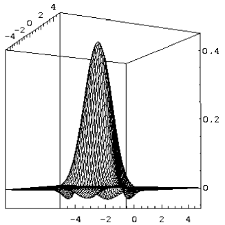
Figure 1: The K–R distribution function for the vacuum state $|0\rangle$.

Figure 1 shows the real part of the expression given by Eq. (47). In accord with the previous description, it is a Gaussian function in position and momentum, modulated by the plane wave phase factor $\cos[2\mathrm{Re}(\alpha)\mathrm{Im}(\alpha)]$.

Formula for K–R distribution of the one photon Fock state $|1\rangle$ is given by

$$K_{|1\rangle\langle 1|}(\alpha,1)=\frac{\sqrt{2}(\alpha^{2}-{\alpha^{\star}}^{2})}{\pi}\times$$

$$\exp\left(-|\alpha|^{2}-\frac{\alpha^{2}}{2}+\frac{(\alpha^{\star})^{2}}{2}\right).$$

The real part of this equation is shown in the Fig. 2. The difference between expressions for the K–R function of the vacuum state and the one photon state is an additional multiplicative amplitude $iqp$ of the oscillating phase factor. This amplitude comes from the product of the one photon wave functions in momentum and position representations, respectively.

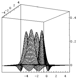
Figure 2: The K–R distribution function for the one photon Fock state.

VI.2 Superposition of coherent states

Another simple but interesting and instructive example that we shall study is a superposition of two coherent states $N(|\alpha_{0}\rangle+|-\alpha_{0}\rangle)$. For this state, from Eq. (24) we derive:

$$K(\alpha,\sigma)=\frac{2N}{\pi\sqrt{1+\sigma\,^{2}}}\;\left[e^{\frac{[\sigma(\alpha^{\star}-\alpha_{0}^{\star})^{2}-\sigma(\alpha-\alpha_{0})^{2}-2|\alpha-\alpha_{0}|^{2}]}{1+\sigma\,^{2}}}\right.$$

$$+e^{\frac{[\sigma(\alpha^{\star}+\alpha_{0}^{\star})^{2}-\sigma(\alpha+\alpha_{0})^{2}-2|\alpha+\alpha_{0}|^{2}]}{1+\sigma\,^{2}}}$$

$$+\left.e^{-2|\alpha_{0}|^{2}}\left(e^{\frac{[\sigma(\alpha^{\star}+\alpha_{0}^{\star})^{2}-\sigma(\alpha-\alpha_{0})^{2}-2(\alpha^{\star}+\alpha_{0}^{\star})(\alpha-\alpha_{0})]}{1+\sigma\,^{2}}}\right.\right.$$

$$+\left.\left.e^{\frac{[\sigma(\alpha^{\star}-\alpha_{0}^{\star})^{2}-\sigma(\alpha+\alpha_{0})^{2}-2(\alpha^{\star}-\alpha_{0}^{\star})(\alpha+\alpha_{0})]}{1+\sigma\,^{2}}}\right)\right],$$ (48)

where

$$N=\Big{(}2+2e^{-2\mid\alpha_{0}\mid^{2}}\Big{)}^{-\frac{1}{2}}.$$

Besides terms corresponding to two individual coherent states there is an interference cross term. Its localization changes with the change of parameter $\sigma$ in the same way as for the superposition of two plane waves. This is illustrated in Fig. 3, where we have plotted the real part of Eq. (48) for $\alpha_{0}=3$ and several values of parameter $\sigma$. We present the real part of distributions rather then the imaginary part (that does not contribute to marginals), or the absolute value (in which no oscillations appear). In Fig. 4 we present the same functions using contour plots. In this representation it is apparent how oscillating interference term moves with the change of the value of the parameter $\sigma$. As was the case of the superposition of plane waves, for $\sigma=0$ interference term is located exactly between the terms that do not correspond to the interference. With the increase of the value of the parameter $\sigma$ interference terms split away and move along ${\mathrm{Re}}(\alpha)$ axis, as they are centered around phase space points $({\mathrm{Re}}(\alpha),{\mathrm{Im}}(\alpha))=(\pm\sigma\alpha_{0},0)$. Again, for $\sigma=1$ oscillating interference terms overlap the terms corresponding to the two individual coherent states. As we have already mentioned, the K–R distribution function is a special case of a distribution which is always equal to zero when wave function is zero at certain point.

Figure 5 shows the same distribution functions when the initial state is rotated in phase space. As an example we have chosen previous initial state rotated by $\varphi=\frac{\pi}{4}$ in phase space, i.e. $\alpha_{0}=3\;e^{i\frac{\pi}{4}}$. The Wigner function of a “rotated state” is simply the rotated Wigner function. This property is the basis for tomography of the Wigner function. By contrast, for other distributions (with parameter $\sigma\neq 0$) this simple relation does not hold, and tomography would not work.

Let us consider behavior of the terms corresponding to the individual coherent states in Fig. 5. Although the center of such a term is located exactly in this point of phase space where coherent state is centered, closer examination tell us that whole term is not “rotated” but rather “shifted” by appropriate values parallel to the coordinate axes. It is clearly seen that for $\sigma\neq 0$ generalized K–R distribution functions single out $p$ and $q$ axes as compared to the other directions in phase space. Interference terms are just rotated but in the opposite direction.

a)
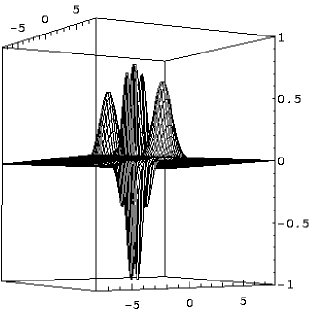
b)
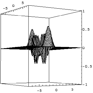
c)

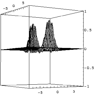
Figure 3: Generalized K–R distribution function of superposition of two coherent states $N(|\alpha_{0}\rangle+|-\alpha_{0}\rangle)$. Here we have chosen $\alpha_{0}=3$, and a) $\sigma=0$ (the Wigner distribution function), b) $\sigma=0.5$, c) $\sigma=1$ (the K–R distribution function).

  
  
a)
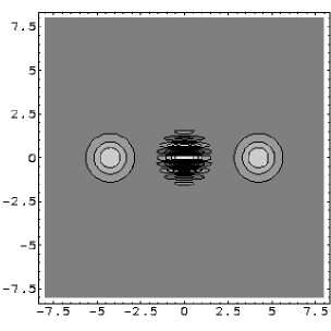
b)
  
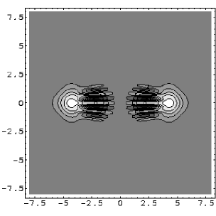
c)

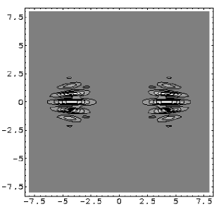
Figure 4: Contour plots of generalized K–R distribution function of superposition of two coherent states $N(|\alpha_{0}\rangle+|-\alpha_{0}\rangle)$. Here we have chosen $\alpha_{0}=3$, and a) $\sigma=0$ (the Wigner distribution function), b) $\sigma=0.5$, c) $\sigma=1$ (the K–R distribution function).

a)
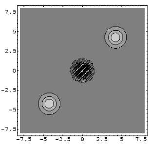
b)
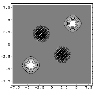
c)

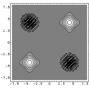
Figure 5: Contour plots of generalized K–R distribution function of superposition of two coherent states $N(|\alpha_{0}\rangle+|-\alpha_{0}\rangle)$. Here we have chosen $\alpha_{0}=3+i3$, and a) $\sigma=0$ (the Wigner distribution function), b) $\sigma=0.5$, c) $\sigma=1$ (the K–R distribution function).

 
$\xi=0.1$

 
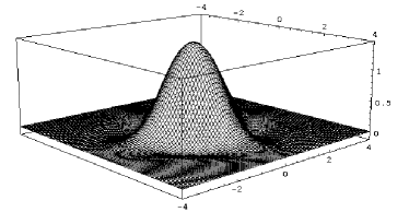
$\xi=0.5$

 
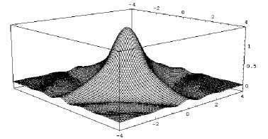
$\xi=0.7$

 
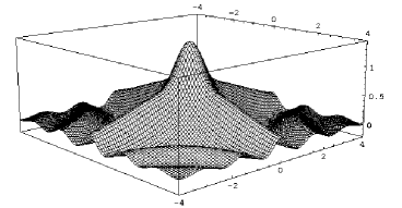
$\xi=0.9$

 
 

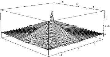
Figure 6: The K–R distribution function of superposition of two squeezed coherent states ${\cal N}(|\xi\rangle+|-\xi\rangle)$.

VI.3 Superposition of coherent squeezed states

In the previous section we have connected the real part of the K–R function with the expectation value of off-diagonal elements of density matrix corresponding to superposition of two infinitely squeezed coherent states. It is interesting to see how K–R distribution evolves if we change the squeezing parameter.

In Fig. 6 we have plotted the real part of the K–R distribution function of superposition of squeezed vacuum states ${\cal N}(|\xi\rangle+|-\xi\rangle)$ for several values of squeezing parameter $\xi$. The K–R distribution apparently shows that an investigated state consist of two perpendicularly squeezed states. Obviously, the closer parameter $\xi$ gets to unity, the more significant are effects of squeezing. Moreover, also basic properties of K–R distribution are emphasized with the increase of the value of the parameter $\xi$: the oscillating $\cos[2\mathrm{Re}(\alpha)\mathrm{Im}(\alpha)]$-like structure is more and more distinct. As we have mentioned before, the K–R distribution single out $p$ a $q$ axes from other phase space directions. Looking at the changes caused by the increase of squeezing, one gets easily convinced of a close connection between the K–R distribution and a superposition of infinitely squeezed coherent states.

VII Summary

We have presented a new class of phase space quasi-distribution functions with correct momentum and position marginal properties, that contains the Wigner distribution function and the K–R distribution as special cases. We have shown how quantum interference appears in phase space if such functions are used for its investigation. In particular, we have focused on similarities and differences between the Wigner function and the K–R distribution.

We have emphasized the most important properties of the K–R distribution function: the fact that this function fully characterizes the quantum state; that the K–R function corresponds to the anti-standard ordering of $\hat{q}$ and $\hat{p}$ operators; and that the real part of K–R distribution is in natural way connected to coherent squeezed states.

Most of the properties of the generalized K–R distribution function we have presented using the formalism of coherent states with the full analogy to the Glauber and Cahill s-ordered quasi-distributions.

References

- (1) E. Wigner, Phys. Rev. 40, 749 (1932)
- (2) K. E. Cahill and R.J. Glauber, Phys. Rev. 177, 1857, 1882 (1969)
- (3) R. J. Glauber, Phys. Rev. Lett. 10, 84 (1963)
- (4) E. C. G Sudarshan, Phys. Rev. Lett. 10, 277 (1963)
-
(5)
K. Husimi, Proc. Phys. Math. Soc. Japan, 22, 246 (1940)
K. Takahashi, Suppl. Prog. Theor. Phys. 98, 109 (1989) - (6) J. G. Kirkwood, Phys. Rev. 44, 31 (1933)
- (7) A. N. Rihaczek, IEEE Trans. Inf. Theory 14, 369 (1968)
- (8) B-G Englert, J. Phys. A, 22, 625 (1989)
- (9) J. Zak, Phys. Rev. A 45, 3540 (1992)
- (10) R. F. O’Connell and E. P. Wigner, Phys. Lett. A vol 83 no 4 (1981), 145
- (11) W. P. Schleich, Quantum Optics in Phase Space, WILEY-VCH (2001).
- (12) L. Cohen, Proceedings of the IEEE 77, No. 7 (1989).
- (13) L. Cohen, Time-Frequency Analysis, PRENTICE HALL (1995).
- (14) H. Margenau, R. N. Hill, Prog. Theor. Phys., 26, 722 (1961)
- (15) L. Praxmeyer, K. Wódkiewicz, Hydrogen atom in the Kirkwood–Rihaczek representation (in preparation)
- (16) L. Cohen, J. Math. Phys. 7, 781 (1966)
- (17) L. Cohen and Y.I. Zaparovanny, J. Math. Phys. 21, 794 (1990)
- (18) G. S. Agarwal and E. Wolf, Phys. Rev. D 2, 2161, 2187, 2206 (1970)
- (19) D. F. Walles, G. J. Milburn, Quantum Optics, SPRINGER–VERLAG (1994)