Chapter 0 Non-classical Gaussian states in noisy environments

Stefan Scheel and Dirk–Gunnar Welsch Stefan Scheel  and Dirk–Gunnar Welsch 

1 Introduction

Research in the field of quantum information theory nowadays focusses more and more on the possibilities of practical implementation of quantum information processes. One of the most promising attempts has seemed to be the usage of entangled Gaussian states since they are rather easy to produce with optical means. In this article we will review properties of Gaussian states and describe operations on them. The interaction of the electromagnetic field with an absorbing dielectric as a special type of environmental interaction will serve as the basis for the understanding of decoherence and entanglement degradation of Gaussian states of light propagating through fibers.

In Section 2 we shortly review the definition of Gaussian states and operations that can be performed on them. These includes symplectic (unitary) transformations, trace-preserving maps, and projective measurements. The important definitions of classicality, separability, and entanglement are defined and appropriate measures are given for them. In Section 3 we review some results on entanglement degradation in dielectric environments. We discuss the decoherence of Gaussian quantum states of light transmitted through absorbing dielectric objects such as fibers. Section 4 is devoted to the study of quantum teleportation in noisy environments. Special emphasis is put onto the question of choosing the correct displacement on the receiver’s side.

2 Gaussian states and Gaussian operations

To begin with, we define Gaussian states and Gaussian operations and discuss some important properties such as non-classicality, separability, and entanglement. A quantum state is called Gaussian if its characteristic function, and hence an appropriately chosen phase-space function, is an exponential form that is at most quadratic in its canonical variables. Most importantly, a Gaussian state is fully characterized by the first and second moments of the $2N$ canonical variables $\,\hat{\!\mbox{\boldmath$\xi$}}{{}^{\rm T}}$ $\!=$ $\!(\hat{x}_{1},\hat{p}_{1},\ldots,\hat{x}_{N},\hat{p}_{N})$ obeying the canonical commutation relations ($\hbar$ $\!=$ $\!1$)

$$\left[\hat{\xi}_{i},\hat{\xi}_{j}\right]=i\Sigma_{ij},$$ (1)

where $\Sigma$ is the $2N$-dimensional symplectic matrix

$$\mbox{\boldmath$\Sigma$}=\left(\begin{array}[]{cc}0&1\\ -1&0\end{array}\right)^{\oplus N}.$$ (2)

This definition seems to suggest that higher moments do not play any rôle. However, this is not correct, since all higher moments can be derived from first and second moments. The first moments describe the position $\kappa$ of the ‘centre-of-mass’ of the Gaussian function in phase-space, whereas the second moments describe the fluctuations of the canonical variables or equivalently, the width of the Gaussian in phase-space. They can be collected in the positive symmetric $2N\times 2N$-dimensional covariance matrix $\Gamma$, viz.

$$\Gamma_{ij}=2\mbox{Tr}\!\left[\bigl{(}\hat{\xi}_{i}-\langle\hat{\xi}_{i}\rangle\bigr{)}\bigl{(}\hat{\xi}_{j}-\langle\hat{\xi}_{j}\rangle\bigr{)}\hat{\varrho}\right]-i\Sigma_{ij}.$$ (3)

The associated charateristic function is the Fourier transform of the Wigner function. Note that without the term $-i\Sigma_{ij}$ one would obtain the covariance matrix corresponding to the density operator in normal order. The fluctuations, however, are not independent from each other. This means that not every positive $2N\times 2N$-dimensional matrix is an admissible covariance matrix, i.e. describes a physical state. The reason for this behaviour is the simple fact that the fluctuations have to obey the Heisenberg uncertainty relations which in matrix form read as

$$\mbox{\boldmath$\Gamma$}+i\mbox{\boldmath$\Sigma$}\geq 0.$$ (4)

With the above definitions we can write the characteristic function of a general Gaussian state as

$$\chi(\mbox{\boldmath$\lambda$})=\exp\left[-{\textstyle\frac{1}{4}}\mbox{\boldmath$\lambda$}^{\rm T}\mbox{\boldmath$\Gamma$}\mbox{\boldmath$\lambda$}+i\mbox{\boldmath$\lambda$}^{\rm T}\mbox{\boldmath$\Sigma$}\mbox{\boldmath$\kappa$}\right].$$ (5)

For the following discussion we will focus on the second moments only. We can transform Gaussian states into each other by transforming the covariance matrix as $\Gamma$ $\!\to$ $\!\mbox{\boldmath$\Gamma$}^{\prime}$ $\!=$ $\!\textbf{S}\mbox{\boldmath$\Gamma$}\textbf{S}^{\rm T}$, where the matrix S has to be chosen such that the canonical commutation relations (1) are fulfilled. This requirement leads to the constraint $\textbf{S}\mbox{\boldmath$\Sigma$}\textbf{S}^{\rm T}$ $\!=$ $\Sigma$. On the level of states, these matrices generate unitary transformations $\hat{\varrho}$ $\!\to$ $\!\hat{\varrho}^{\prime}$ $\!=$ $\!\hat{U}(\textbf{S})\hat{\varrho}\hat{U}^{\dagger}(\textbf{S})$. In turn, any unitary transformation which is bilinear in the canonical variables can be described by a symplectic matrix. All symplectic matrices S form the (non-compact) symplectic group Sp($2N$,$\mathbb{R}$). As for every group, it has certain normal forms associated with it. One of the most important ones is the generalized Euler decomposition [2]: Every symplectic matrix S can be decomposed into three factors, $\textbf{S}=\textbf{O}_{1}\textbf{D}\textbf{O}_{2}$, where the $\textbf{O}_{i}$ belong to the $N$-dimensional (compact) orthogonal group and D is a diagonal matrix with entries $(k_{1},1/k_{1},\ldots,k_{N},1/k_{N})$. This decomposition has an immediate physical interpretation: The $\textbf{O}_{i}$ generate $N$-mode rotations (generated by beam splitter networks and phase shifters) and the matrix D describes single-mode squeezings.

1 Classicality

A very special feature of a quantum state is its possible non-classical character, which means that its inherent statistics cannot be modelled by a classical probability distribution. A widely used definition has been given by Titulaer and Glauber [3] saying that a state is classical (or ‘predetermined’ in their words) if and only if its $P$ function is positive semi-definite and sufficiently smooth, hence $P\in L_{2}(\mathbb{R}^{+})$. This definition has recently been translated into a measurable criterion which is based on quadrature distributions [4].

Let us discuss the implications for a general Gaussian $N$-mode state. The main result is that we regard a Gaussian state as non-classical whenever one or more eigenvalues of its covariance matrix drop below $1$. The reasoning behind the argument is that in such a case the characteristic function does not possess a Fourier transform since it increases exponentially at infinity. To answer the question of whether a Gaussian state is classical or not, we recall that any Gaussian state (with zero mean) can be generated by acting on a thermal state (being classical) with a symplectic matrix S. That is, we can start with a covariance matrix of the form $\mbox{\boldmath$\Gamma$}_{\rm th}$ $\!=$ $\!2\mbox{diag}(n_{1},n_{1},\ldots,n_{N},n_{N})$ $\!+$ 1, with $n_{i}$ being the mean thermal excitation number in the $i$-th mode. Next we act on $\mbox{\boldmath$\Gamma$}_{\rm th}$ with a symplectic matrix S and compute the eigenvalues of the transformed covariance matrix $\textbf{S}\mbox{\boldmath$\Gamma$}_{\rm th}\textbf{S}^{\rm T}$ with S $\!=$ $\!\textbf{O}_{1}\textbf{D}\textbf{O}_{2}$.

To give a simple example, let us consider a single-mode Gaussian state. The sought eigenvalues are simply the eigenvalues of the covariance matrix ($k$ $\!=$ $\!e^{\zeta}$)

$$\textbf{D}\mbox{\boldmath$\Gamma$}_{\rm th}\textbf{D}=\textrm{diag}\left[e^{2\zeta}(2n+1),e^{-2\zeta}(2n+1)\right]$$ (6)

(the orthogonal matrices $\textbf{O}_{i}$ do not play a rôle here), from which we immediately find the well-known relation $|\zeta_{\max}|$ $\!=$ $\!\frac{1}{2}\ln(2n+1)$ for the maximal squeezing value such that the state stays classically [5]. We see that a state can be classical, though it is squeezed. Needless to say that multimode Gaussian states can be treated in the same way. Clearly, the number of parameters one can choose increases rapidly.

Furthermore, a non-classicality measure $C(\hat{\varrho})$ based on the relative entropy can be defined as

$$C(\hat{\varrho})=\min_{\hat{\sigma}_{\rm class.}}\mbox{Tr}\left[\hat{\varrho}\left(\ln\hat{\varrho}-\ln\hat{\sigma}\right)\right].$$ (7)

The advantage of using this entropic measure for Gaussian states is that it can be easily calculated [6]. Note that this measure can be equally well used as the measure based on Bures’ metric defined in [7].

2 CP maps and partial measurements

Until now we have described unitary operations on the level of states. Decoherence processes, however, correspond to operations in a larger class, the completely positive (CP) maps. Physically, they are unitary operations in a larger Hilbert space (Naimark theorem [8]). A typical example is the interaction with a dissipative environment which is traced out afterwards. On the level of covariance matrices, CP maps act as

$$\mbox{\boldmath$\Gamma$}\to\mbox{\boldmath$\Gamma$}^{\prime}=\mbox{\boldmath$A$}\mbox{\boldmath$\Gamma$}\mbox{\boldmath$A$}^{\rm T}+\mbox{\boldmath$G$},$$ (8)

where $G$ is a positive symmetric matrix and $A$ an arbitrary matrix, with the only constraint being that the resulting matrix $\mbox{\boldmath$\Gamma$}^{\prime}$ should be a valid covariance matrix, i.e. fulfils Eq. (4). The non-orthogonality of the matrix $A$ is a direct consequence of dissipation, and $G$ is the additional noise as required by the dissipation-fluctuation theorem. As a simple example, $G$ can represent pure thermal noise. In this case, one can produce a thermal state with covariance matrix $\mbox{\boldmath$\Gamma$}_{\rm th}$ $\!=$ $\!(2n$ $\!+$ $\!1)\textbf{1}$ from the vacuum with $\mbox{\boldmath$\Gamma$}_{\rm vac}$ $\!=$ 1 with the help of the matrices $A$ $\!=$ 1 and $G$ $\!=$ $\!2n\textbf{1}$.

Another important class of operations is generated by (homodyne) measurements on subsystems. For that, let us write the covariance matrix of a bipartite system in block form $\Gamma$ $\!=$ $\!\left(\begin{array}[]{cc}\textbf{C}_{1}&\textbf{C}_{3}\\ \textbf{C}_{3}^{\rm T}&\textbf{C}_{2}\end{array}\right)$ where $\textbf{C}_{1}$ and $\textbf{C}_{2}$ are the principal submatrices with respect to the subsystems $1$ and $2$, respectively, and $\textbf{C}_{3}$ is the correlation matrix between the subsystems. In general, the dimension of all these matrices can be different, e.g., $\textbf{C}_{1}$ is $2N\times 2N$, $\textbf{C}_{2}$ is $2M\times 2M$, and $\textbf{C}_{3}$ is $2N\times 2M$. Projection measurements on subsystem $2$ onto a Gaussian state with covariance matrix D leads to the Schur complement [9] with respect to the leading principal submatrix $\textbf{C}_{1}$,

$$\mbox{\boldmath$\Gamma$}\to\mbox{\boldmath$\Gamma$}^{\prime}=\textbf{C}_{1}-\textbf{C}_{3}\left(\textbf{C}_{2}+\textbf{D}^{2}\right)^{-1}\textbf{C}_{3}^{\rm T}.$$ (9)

The probability of measuring a certain outcome is $\bigl{[}\det\,\big{(}\textbf{C}_{2}$ $\!+$ $\!\textbf{D}^{2}\big{)}\bigr{]}^{-1/2}$. Note that the dimension of the matrix $\mbox{\boldmath$\Gamma$}^{\prime}$ is now reduced. When D is the identity matrix, then the transformation (9) describes vacuum projection. For D $\!=$ $\!\lim_{d\to 0}(1/d,d,\ldots,1/d,d)$ it describes homodyne detection, in which case the inverse has to be thought of as the Moore–Penrose (MP) inverse [10]. An analogous treatment has to be made for the corresponding determinant. Combining the transformations (8) and (9) gives the most general (not necessarily trace-preserving) Gaussian operation where the name means that they leave the Gaussian character of a state invariant.

3 Separability and entanglement

So far, we have discussed general features of Gaussian states and Gaussian operations. In what follows, we will focus on bipartite Gaussian states and their entanglement properties. To be more precise, we restrict ourselves to the class of ($1\times 1$)-mode states, in which one mode of the electromagnetic field is entangled with another one. The covariance matrix $\Gamma$ is thus a ($4\times 4$)-matrix. In order to check whether a given bipartite Gaussian state is entangled or not, a necessary and sufficient separability criterion has been developed [11, 12]. It is equivalent to the Peres–Horodecki criterion for entangled qubits [13]. The test consists of checking whether the partial transpose of the density operator is again a valid density operator. In this case, the state is separable and therefore not entangled. On the level of the covariance matrix, the partial transpose consists of pre- and post-multiplying $\Gamma$ by the diagonal matrix P $\!=$ $\!\mbox{diag}(1,1,1,-1)$, viz. $\mbox{\boldmath$\Gamma$}^{\rm P.T.}$ $\!=$ $\!\textbf{P}\mbox{\boldmath$\Gamma$}\textbf{P}^{\rm T}$. Hence, if $\mbox{\boldmath$\Gamma$}^{\rm P.T.}$ $\!+$ $\!i\mbox{\boldmath$\Sigma$}$ $\!\geq$ $\!0$ the state is separable. In the block notation used in Section 2, this criterion translates as [12]

$$\det\textbf{C}_{1}\textbf{C}_{2}+\big{(}1-|\det\textbf{C}_{3}|\big{)}^{2}-\mbox{Tr}\left[\textbf{C}_{1}\mbox{\boldmath$\Sigma$}\textbf{C}_{3}\mbox{\boldmath$\Sigma$}\textbf{C}_{2}\mbox{\boldmath$\Sigma$}\textbf{C}_{3}^{\rm T}\mbox{\boldmath$\Sigma$}\right]\geq\det\textbf{C}_{1}+\det\textbf{C}_{2}\,.$$ (10)

Once one has checked for inseparability, one may ask how much entangled the state is. This answer is given by computing the logarithmic negativity [14], so far the only computable measure for states in infinite-dimensional Hilbert spaces. It is defined as the sum of the symplectic eigenvalues of $\mbox{\boldmath$\Gamma$}^{\rm P.T.}$, which translates as [9]

$$E_{N}(\hat{\varrho})=\left\{\begin{array}[]{cc}-(\log\circ f)(\mbox{\boldmath$\Gamma$})\,,&\mbox{if }f(\mbox{\boldmath$\Gamma$})<1,\\[2.15277pt] 0&\mbox{otherwise},\end{array}\right.$$ (11)

where

$$f(\mbox{\boldmath$\Gamma$})=\left({\textstyle\frac{1}{2}}\left(\det\textbf{C}_{1}\!+\!\det\textbf{C}_{2}\right)\!-\!\det\textbf{C}_{3}\!-\!\sqrt{\left[{\textstyle\frac{1}{2}}(\det\textbf{C}_{1}\!+\!\det\textbf{C}_{2})\!-\!\det\textbf{C}_{3}\right]^{2}-\det\mbox{\boldmath$\Gamma$}}\right)^{1/2}.$$ (12)

An immediate consequence is that it is impossible to distill Gaussian states with Gaussian operations [9, 15]. We are now in the position to look at practically important situations such as entanglement degradation and quantum teleportation in noisy environments.

3 Entanglement degradation

Let us consider the influence of passive optical devices on entangled two-mode quantum states. We have seen in the previous section that Gaussian states are fully characterized by their (first and) second moments. In order to describe the influence of dielectric objects on the quantum state we therefore need to know only how these moments transform. The easiest way to see this is to look at the quantum-optical input-output relations [16, 17]. They relate the amplitude operators of the electromagnetic field impinging on the dielectric object to the amplitude operators of the field leaving the device. In the following we will assume that the dielectric material shows absorption as it is generically the case. This is due to the fact that the dielectric permittivity (as well as the magnetic susceptibility) has to fulfil the Kramers–Kronig relations, which connect the real part of the permittivity (responsible for dispersion) to the imaginary part (responsible for absorption). That said one recognizes that quantization of the electromagnetic field in absorbing matter has to be performed.

Here we will use the macroscopic description [16, 18] that is most suitable for the situation we have in mind. The electromagnetic field is quantized by expanding it in terms of a complete set of bosonic vector fields $\hat{\textbf{f}}(\textbf{r},\omega)$ that describe collective excitations of the electromagnetic field, the matter polarization, and the reservoir responsible for absorption, viz.

$$\hat{\textbf{E}}(\textbf{r})=i\sqrt{\frac{\hbar}{\pi\varepsilon_{0}}}\int d^{3}{s}\int\limits_{0}^{\infty}d\omega\,\frac{\omega^{2}}{c^{2}}\,\sqrt{{\rm Im}\,\varepsilon(\textbf{s},\omega)}\mbox{\boldmath$G$}(\textbf{r},\textbf{s},\omega)\,\hat{\textbf{f}}(\textbf{s},\omega)+\mbox{H.c.}\,,$$ (13)

with $\mbox{\boldmath$G$}(\textbf{r},\textbf{s},\omega)$ being the classical Green tensor. Expanding the electromagnetic field in terms of amplitude operators outside the dielectric device where no matter is present, one can derive the input-output relation

$$\hat{\textbf{b}}(\omega)=\textbf{T}(\omega)\hat{\textbf{a}}(\omega)+\textbf{A}(\omega)\hat{\textbf{g}}(\omega)$$ (14)

in which the $\hat{a}_{i}(\omega)$ and $\hat{b}_{i}(\omega)$ ($i$ $\!=$ $\!1,2$) denote the amplitude operators of the incoming and outgoing fields at frequency $\omega$, and the $\hat{g}_{i}(\omega)$ denote the noise operators associated with absorption inside the device. The matrices $\textbf{T}(\omega)$ and $\textbf{A}(\omega)$ are the transformation and absorption matrices, respectively. They are determined by the Green tensor and satisfy the (energy-)conservation relation $\textbf{T}(\omega)\textbf{T}^{+}(\omega)$ $\!+$ $\!\textbf{A}(\omega)\textbf{A}^{+}(\omega)$ $\!=$ 1. With regard to Gaussian states, we need to know how second moments of the amplitude operators transform. Assuming that the incoming field modes and the device are not correlated, we derive, for example,

$$\langle\hat{b}_{1}^{\dagger}(\omega)\hat{b}_{1}(\omega)\rangle = |T_{11}(\omega)|^{2}\langle\hat{a}_{1}^{\dagger}(\omega)\hat{a}_{1}(\omega)\rangle+|T_{12}(\omega)|^{2}\langle\hat{a}_{2}^{\dagger}(\omega)\hat{a}_{2}(\omega)\rangle$$ (15)

$$+\,|A_{11}(\omega)|^{2}\langle\hat{g}_{1}^{\dagger}(\omega)\hat{g}_{1}(\omega)\rangle+|A_{12}(\omega)|^{2}\langle\hat{g}_{2}^{\dagger}(\omega)\hat{g}_{2}(\omega)\rangle.$$

Let us now look at the most generic two-mode entangled Gaussian state, the two-mode squeezed vacuum (TMSV). In the Fock basis it reads ($\zeta\in\mathbb{R}^{+}$)

$$|\mbox{TMSV}\rangle=\exp\zeta(\hat{a}_{1}\hat{a}_{2}-\hat{a}_{1}^{\dagger}\hat{a}_{2}^{\dagger})|00\rangle=\sqrt{1-q^{2}}\sum\limits_{n=0}^{\infty}q^{n}|nn\rangle\,,\quad q=\tanh\zeta\,.$$ (16)

It is separable only if $q$ $\!=$ $\!0$, otherwise it is entangled, where the entanglement content is $E$ $\!=$ $\!-\ln(1-q^{2})$ $\!-$ $\!q^{2}/(1-q^{2})\ln q^{2}$ $\lesssim 2\zeta$ $\!=$ $\!E_{N}$. In the language used in Section 2, the TMSV translates into a covariance matrix

$$\mbox{\boldmath$\Gamma$}=\left(\begin{array}[]{rrrr}c&0&s&0\\ 0&c&0&-s\\ s&0&c&0\\ 0&-s&0&c\end{array}\right),\quad c=\cosh 2\zeta,\quad s=\sinh 2\zeta.$$ (17)

We are interested how the entanglement changes when the two modes are transmitted through two fibers with equal transmission coeffcients $|T|$, reflection coefficients $|R|$, and mean thermal photon numbers $n_{\rm th}$. Applying the input-output relations (14), the second moments transform as

$$c\to c|T|^{2}+|R|^{2}+(2n_{\rm th}+1)(1-|T|^{2}-|R|^{2})\,,\quad s\to s|T|^{2},$$ (18)

which translates into a transformation of the covariance matrix as

$$\mbox{\boldmath$\Gamma$}\to|T|^{2}\mbox{\boldmath$\Gamma$}+\left[|R|^{2}+(2n_{\rm th}+1)(1-|T|^{2}-|R|^{2})\right]\textbf{1},$$ (19)

from which we can easily identify the matrices $A$ and $G$ in the transformation (8). Note that we have not taken care about local phases since they do not play any rôle in determining separability and entanglement. Applying the criterion (10) to the covariance matrix (19), we can easily rewrite the condition of separability as [19]

$$n_{\rm th}\geq\frac{|T|^{2}(1-e^{-2\zeta})}{2(1-|R|^{2}-|T|^{2})}\,.$$ (20)

Restricting ourselves to vanishing incoupling losses ($R$ $\!=$ $\!0$) and imposing the Lambert–Beer law of extinction $|T|$ $\!=$ $\!e^{-l/l_{A}}$, with $l_{A}$ being the characteristic absorption length of the fibers, from Eq. (20) we derive for the fiber length after which the TMSV becomes separable $l_{S}=\frac{1}{2}l_{A}\ln[1+(1-e^{-2\zeta})/2n_{\rm th}]$. These results say that for fibers at zero temperature entanglement will always be present (although possibly arbitrarily small). For finite $n_{\rm th}$ the separability length $l_{S}$ is a function of the squeezing parameter $\zeta$ of the input state.

Let us now look at the actual entanglement content in terms of the logarithmic negativity. Again, we only need to insert the transformed covariance matrix (19) into Eq. (11). Neglecting again the mean thermal photon numbers of the fibers ($n_{\rm th}=0$), we derive for the logarithmic negativity

$$E_{N}=-\ln\left[1-|T|^{2}(1-e^{-2\zeta})\right],$$ (21)

which is independent of the reflection coefficient $R$. For perfect transmission ($T$ $\!=$ $\!1$), we obtain the familiar result $E_{N}$ $\!=$ $\!2\zeta$. Another immediate consequence of Eq. (21) is that the transmittable entanglement saturates. In the limit of infinite initial squeezing ($\zeta$ $\!\to$ $\!\infty$) the maximal entanglement that can pass through fibers of given length $l$ is just $E_{N,\max}$ $\!=$ $\!-$ $\!\ln\bigl{[}1$ $\!-$ $\!|T|^{2}\bigr{]}$ $\!=$ $\!-$ $\!\ln\bigl{[}1$ $\!-$ $\!e^{-2l/l_{A}}\bigr{]}$. In other words, no matter how strong the initial squeezing was, the amount of transmittable entanglement is limited by the fiber properties (in this simple model the fiber length normalized to the characteristic absorption length). Moreover, the entanglement depends in a simple manner on the overall losses (accounting for reflection and absorption, since $1$ $\!-$ $\!|T|^{2}$ $\!=$ $\!|R|^{2}$ $\!+$ $\!|A|^{2}$) during transmission. Figure 2 shows the dependence of the maximal entanglement on the fiber length. It says that in order to transmit the quantum information equivalent to $E_{N}$ $\!=$ $\!1$, the transmission distance must not exceed the value $l$ $\!=$ $\!l_{A}/2\ln 2$ $\!\approx$ $\!0.35\,l_{A}$. Equivalently, the transmission coefficient must not be smaller than $|T|^{2}$ $\!=$ $\!0.5$.

Let us apply this result to quantum dense coding considered, where a classical bit is encoded in a coherent shift of one mode of a TMSV. The result in [20] is that classical coding is superior to quantum dense coding whenever the transmission coefficient $|T|^{2}$ drops below the value of $0.75$, which corresponds, according to Eq. (21), to a log-negativity of $2$. The example clearly shows the limits of the performance of quantum information processes due to the unavoidably existing entanglement degradation.

4 Quantum teleportation in noisy environments

A widely discussed process in quantum information theory has been quantum teleportation [22]. Its purpose is to transport a substantial amount of information about an unknown (single) quantum state spatially from one location to another without transmitting the state itself. The idea is the following. A signal mode that is prepared in the unknown quantum state is mixed with one mode of a (maximally) entangled two-mode state, and the resulting output quantum state is subsequently measured by homodyne detection. The (single-)measurement result is submitted classically to the receiver who, depending on the measurement result, performs a coherent displacement of the quantum state in which his mode (of the two-mode entangled system) has been prepared owing to the measurement.

In order to make contact with the theory developed in the previous sections, we restrict ourselves to the case in which the unknown state is a Gaussian (with zero mean). That is, the initial state in mode 0 can be described by a ($2\times 2$) covariance matrix $\mbox{\boldmath$\Gamma$}_{\rm in}$. This class covers all squeezed and thermal states and combinations of them. Accordingly, the source of the entangled state in modes 1 and 2 is assumed to produce a TMSV with a covariance matrix $\mbox{\boldmath$\Gamma$}_{\rm TMSV}$ as in Eq. (17). The covariance matrix of the total state at the beginning of the teleportation process is then the direct sum $\mbox{\boldmath$\Gamma$}_{\rm in}\oplus\mbox{\boldmath$\Gamma$}_{\rm TMSV}$.

As already mentioned, the transmission lines from the entanglement source to the sender and the receiver, which are realized, e.g., by fibers, are not perfect in practice. The question we would like to address is to what extent the teleportation protocol has to be modified when decoherence is present. Especially, we will try to answer the question where the source of the entangled state has to be located to obtain an optimal teleportation protocol.

1 Imperfect teleportation

Let us slightly generalize the situation, compared to the previous section, in that we consider the possibility of having two different fibers connecting the entanglement source with the sender and the receiver. The matrix $\mbox{\boldmath$\Gamma$}_{\rm TMSV}$ will thus change to [21]

$$\mbox{\boldmath$\Gamma$}_{\rm TMSV}\to\mbox{\boldmath$\Gamma$}_{\rm dec}=\left(\begin{array}[]{rrrr}a&0&c_{1}&c_{2}\\ 0&a&c_{2}&-c_{1}\\ c_{1}&c_{2}&b&0\\ c_{2}&-c_{1}&0&b\end{array}\right)\equiv\left(\begin{array}[]{ll}\textbf{A}&\textbf{C}\\ \textbf{C}^{\rm T}&\textbf{B}\end{array}\right)$$ (22)

with

$$a = c|T_{1}|^{2}+|R_{1}|^{2}+(2n_{{\rm th},1}+1)(1-|T_{1}|^{2}-|R_{1}|^{2}),$$ (23)

$$b = c|T_{2}|^{2}+|R_{2}|^{2}+(2n_{{\rm th},2}+1)(1-|T_{2}|^{2}-|R_{2}|^{2}),$$ (24)

$$c_{1} = s\textrm{Re}(T_{1}T_{2}),$$ (25)

$$c_{2} = s\textrm{Im}(T_{1}T_{2}).$$ (26)

Here, the $T_{i}$ and $R_{i}$ ($i$ $\!=$ $\!1,2$) are the transmission and reflection coefficients of the $i$th fiber.

The operation of mixing one mode of the transmitted TMSV (covariance matrix $\mbox{\boldmath$\Gamma$}_{\rm dec}$) with the signal mode at a symmetric beam splitter is described by a symplectic matrix of the form

$$\textbf{S}_{\rm BS}=\frac{1}{\sqrt{2}}\left(\begin{array}[]{rr}\textbf{1}&\textbf{1}\\ -\textbf{1}&\textbf{1}\end{array}\right)\,.$$ (27)

Remembering that $\textbf{S}_{\rm BS}$ acts only on modes 0 and 1, the covariance matrix of the tripartite state reads as $\mbox{\boldmath$\Gamma$}_{012}$ $\!=$ $\!(\textbf{S}_{\rm BS}\oplus\textbf{1}_{2})$ $(\mbox{\boldmath$\Gamma$}_{\rm in}\oplus\mbox{\boldmath$\Gamma$}_{\rm dec})(\textbf{S}_{\rm BS}\oplus\textbf{1}_{2})^{\rm T}$, where $\textbf{1}_{2}$ is the identity operation on mode 2, the receiver’s side. In block matrix notation, $\mbox{\boldmath$\Gamma$}_{012}$ reads

$$\mbox{\boldmath$\Gamma$}_{012} = \left(\begin{array}[]{ccc}(\mbox{\boldmath$\Gamma$}_{\rm in}+\textbf{A})/2&(\textbf{A}-\mbox{\boldmath$\Gamma$}_{\rm in})/2&\textbf{C}/\sqrt{2}\\ (\textbf{A}-\mbox{\boldmath$\Gamma$}_{\rm in})/2&(\mbox{\boldmath$\Gamma$}_{\rm in}+\textbf{A})/2&\textbf{C}/\sqrt{2}\\ \textbf{C}^{\rm T}/\sqrt{2}&\textbf{C}^{\rm T}/\sqrt{2}&\textbf{B}\end{array}\right):=\left(\begin{array}[]{ll}\textbf{M}&\textbf{N}\\ \textbf{N}^{\rm T}&\textbf{B}\end{array}\right).$$ (33)

As shown in the Appendix, homodyne detection (with respect to the variables $x_{0}$ and $p_{1}$ after the beam splitter) is equivalent to a partial Fourier transform [Eqs. (A.1) and (A.4)]. Let us denote the measurement outcomes corresponding to the variables $x_{0}$ and $p_{1}$ by $X_{x_{0}}$ and $X_{p_{1}}$, respectively. The characteristic function at the receiver’s side will then be

$$\chi_{\rm rec}(\mbox{\boldmath$\lambda$}_{2})=p(X_{x_{0}},X_{p_{1}})\exp\left[-\frac{1}{4}\mbox{\boldmath$\lambda$}_{2}^{\rm T}\mbox{\boldmath$\Gamma$}_{\rm rec}\mbox{\boldmath$\lambda$}_{2}+i\,\mbox{\boldmath$\lambda$}_{2}^{\rm T}\textbf{N}^{\rm T}(\mbox{\boldmath$\pi$}\textbf{M}\mbox{\boldmath$\pi$})^{\rm MP}\left(\!\begin{array}[]{r}X_{x_{0}}\\ -X_{p_{1}}\end{array}\!\right)\right].$$ (34)

The probability of obtaining a certain pair of measurement outcomes is

$$p(X_{x_{0}},X_{p_{1}})=\frac{1}{\pi\sqrt{\det(\mbox{\boldmath$\pi$}\textbf{M}\mbox{\boldmath$\pi$})}}\exp\!\left[-\begin{array}[]{cc}(\,X_{x_{0}}&-X_{p_{1}}\,)\\ &\end{array}(\mbox{\boldmath$\pi$}\textbf{M}\mbox{\boldmath$\pi$})^{\rm MP}\left(\!\begin{array}[]{r}X_{x_{0}}\\ -X_{p_{1}}\end{array}\!\right)\right],$$ (35)

and the covariance matrix of the receiver’s quantum state obtains the form

$$\mbox{\boldmath$\Gamma$}_{\rm rec}=\textbf{B}-\textbf{N}^{\rm T}(\mbox{\boldmath$\pi$}\textbf{M}\mbox{\boldmath$\pi$})^{\rm MP}\textbf{N},$$ (36)

where $\pi$ $\!=$ $\!\mbox{diag}(0,1,1,0)$ and the superscript MP denotes the Moore–Penrose inverse. The matrix $\pi$ is, in fact, a projector onto the $(p_{0},x_{1})$-plane. It removes all entries of M except the square block matrix specified by the $1$-entries. The Moore–Penrose inverse of a matrix containing a square block on the diagonal and zeros otherwise is nothing but a matrix with the inverse of the square block at the same position (and zero everywhere else).

If we denote the elements of the covariance matrix of the unknown signal state by $\mbox{\boldmath$\Gamma$}_{\rm in}$ $\!=$ $\!\left(\begin{array}[]{cc}x&z\\ z&y\end{array}\right)$, the involved matrices read

$$\textbf{N}=\left(\begin{array}[]{rr}c_{2}&-c_{1}\\ c_{1}&c_{2}\end{array}\right),\quad(\mbox{\boldmath$\pi$}\textbf{M}\mbox{\boldmath$\pi$})^{\rm MP}=\frac{1}{(a+x)(a+y)-z^{2}}\left(\begin{array}[]{cc}a+x&z\\ z&a+y\end{array}\right),$$ (37)

and the covariance matrix (36) thus takes the form of

$$\mbox{\boldmath$\Gamma$}_{\rm rec}=\left(\begin{array}[]{cc}b&0\\ 0&b\end{array}\right)-\frac{1}{(x+a)(y+a)-z^{2}}$$ (43)

$$\times\left(\!\!\begin{array}[]{cc}c_{2}^{2}(x+a)+c_{1}^{2}(y+a)+2c_{1}c_{2}z&c_{1}c_{2}(y-x)-z(c_{1}^{2}-c_{2}^{2})\\ c_{1}c_{2}(y-x)-z(c_{1}^{2}-c_{2}^{2})&c_{1}^{2}(x+a)+c_{2}^{2}(y+a)-2c_{1}c_{2}z\end{array}\!\!\right)\!.$$

In the limit $\zeta\to\infty$, perfect transmission of the TMSV, and the phase adjusted such that $c_{2}$ $\!=$ $\!0$, the covariance matrix on the receiver’s side becomes $\mbox{\boldmath$\Gamma$}_{\rm rec}$ $\!=$ $\!\mbox{\boldmath$\Gamma$}_{\rm in}$. In particular, we recover that for perfect teleportation an infinitely squeezed TMSV (with $\zeta\to\infty$) is needed. Note that $\mbox{\boldmath$\Gamma$}_{\rm rec}$ does not depend on the measurement result, even for non-perfect transmission. That means that the information about the quantum features of a Gaussian state are not transported via the classical channel. What we see, though, is that the covariance matrix is sensitive to the properties of the channel itself.

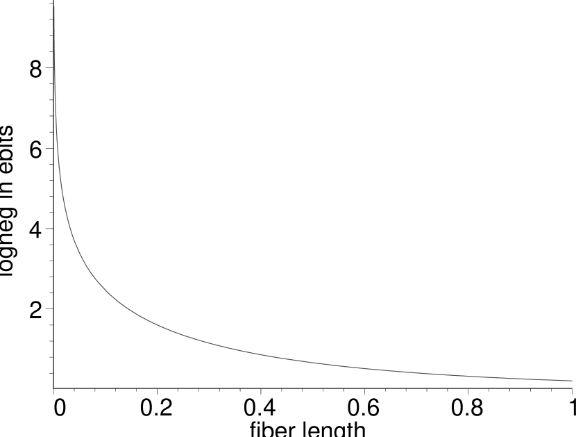
Figure 1: Maximally transmittable entanglement as a function of the fiber length (in units of the absorption length) for the case of a TMSV input.

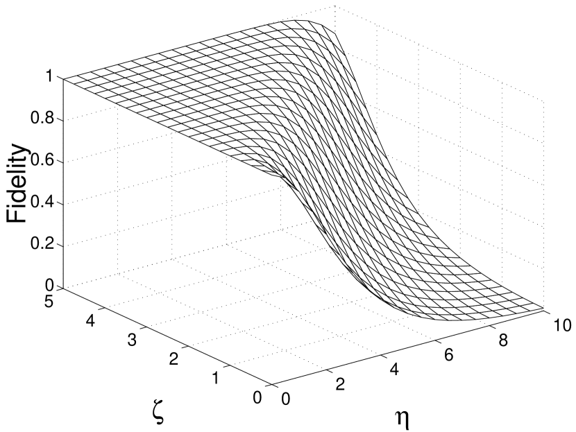
Figure 2: Teleportation fidelity $F_{\rm qu}$ of a (pure) squeezed state (squeezing parameter $\eta$) by means of an unperturbed TMSV (squeezing parameter $\zeta$).

2 Teleportation fidelity

Generically, the TMSV is neither infinitely squeezed nor are the transmission lines from the entanglement source to sender and receiver perfect. Hence, one needs a measure for the success rate of the teleportation protocol. For teleporting pure quantum states, one commonly uses the fidelity defined as the overlap between the quantum state to be teleported and the quantum state at the receiver. In terms of their characteristic functions, the fidelity is given as a double integral over the (complex) parameter $\lambda$ as

$$F=\frac{1}{\pi}\int d^{2}\mbox{\boldmath$\lambda$}\,\chi_{\rm in}(\mbox{\boldmath$\lambda$})\chi_{\rm rec}(-\mbox{\boldmath$\lambda$}).$$ (44)

For Gaussian states with zero mean the negative argument in Eq. (44) does not matter since the characteristic function is an exponential quadratic form of $\lambda$. As we have seen, the homodyne detection introduces a coherent displacement, but does not influence the covariance matrix. With regard to the quantum properties, it is therefore sufficient to compute the overlap between characteristic functions with zero mean. In that way, from Eq. (44) we find that

$$F\to F_{\rm qu}=\frac{2}{\sqrt{\det(\mbox{\boldmath$\Gamma$}_{\rm in}+\mbox{\boldmath$\Gamma$}_{\rm rec})}}\,.$$ (45)

For perfect teleportation, the covariance matrix of the receiver’s state is identical to the covariance matrix of the signal state to be teleported, and the fidelity becomes $F_{\rm qu}$ $\!=$ $\!(\det\mbox{\boldmath$\Gamma$}_{\rm in})^{-1/2}$ $\!=$ $\!1$. Even if entanglement degradation be disregarded, perfect teleportation cannot be realized, because of finite squeezing. Let us consider a (pure) squeezed signal state and disregard entanglement degradation, so that the entangled state is simply the unchanged (pure) TMSV state. The parameters to look at are $a$ $\!=$ $\!b$ $\!=$ $\!c$ $\!=$ $\!\cosh 2\zeta$, $c_{1}$ $\!=$ $\!s$ $\!=$ $\!\sinh 2\zeta$, $c_{2}$ $\!=$ $\!0$, $x$ $\!=$ $\!y$ $\!=$ $\!\cosh\eta$, $z=\sinh\eta$. The teleportation fidelity according to Eq. (45) is then

$$F_{\rm qu}=\sqrt{1-\frac{\sinh^{2}\eta}{(\cosh\eta+\cosh 2\zeta)^{2}}}\equiv\sqrt{1-\frac{\sinh^{2}\eta}{(\cosh\eta+\cosh E_{N})^{2}}}$$ (46)

[cf. Eq. (21)], whose behaviour is illustrated in Fig. 2. We see that for chosen squeezing parameter $\eta$ of the signal state the fidelity is a monotonous function of the inserted entanglement $E_{N}$. In particular, the classical teleportation fidelity (obtained for $\zeta$ $\!=$ $\!0$) is read off as $\sqrt{2/(1+\cosh\eta)}$.

3 Choice of the coherent displacement

There have been some discussions recently about what kind of coherent displacement should be applied [23, 24]. Let us look at Eq. (34). In the limit of an infinitely entangled TMSV the product $\textbf{N}^{\rm T}(\mbox{\boldmath$\pi$}\textbf{M}\mbox{\boldmath$\pi$})^{\rm MP}$ becomes the symplectic matrix $\Sigma$ which is independent of the initial state. Thus, in the ideal case the coherent displacement is solely determined by the measurement results. This is the standard teleportation protocol, where the coherent displacement to be performed on the receivers’s side is exactly $X_{x_{0}}$ $\!-$ $\!iX_{p_{1}}$.

Even if an infinitely entangled TMSV were available, entanglement degradation would prevent one from observing this simple result. On recalling Eq. (37) together with Eqs. (23) and (25), the relevant matrix product $\textbf{N}^{\rm T}(\mbox{\boldmath$\pi$}\textbf{M}\mbox{\boldmath$\pi$})^{\rm MP}$ now reads

$$\lim_{\zeta\to\infty}\textbf{N}^{\rm T}(\mbox{\boldmath$\pi$}\textbf{M}\mbox{\boldmath$\pi$})^{\rm MP}=\frac{1}{|T_{1}|^{2}}\left(\begin{array}[]{rr}\textrm{Im}\left(T_{1}T_{2}\right)&\textrm{Re}\left(T_{1}T_{2}\right)\\ \textrm{Re}\left(T_{1}T_{2}\right)&-\textrm{Im}\left(T_{1}T_{2}\right)\end{array}\right).$$ (47)

If we write the transmission coefficients as $T_{i}$ $\!=$ $\!|T_{i}|e^{i\varphi_{i}}$, Eq. (47) becomes

$$\lim_{\zeta\to\infty}\textbf{N}^{\rm T}(\mbox{\boldmath$\pi$}\textbf{M}\mbox{\boldmath$\pi$})^{\rm MP} = \mbox{\boldmath$\Sigma$}\left|\frac{T_{2}}{T_{1}}\right|\left(\begin{array}[]{rr}\cos\left(\varphi_{1}\!+\!\varphi_{2}\right)&-\sin\left(\varphi_{1}\!+\!\varphi_{2}\right)\\ \sin\left(\varphi_{1}\!+\!\varphi_{2}\right)&\cos\left(\varphi_{1}\!+\!\varphi_{2}\right)\end{array}\right).$$ (50)

We see that, apart from the (irrelevant) phase shift $-(\varphi_{1}$ $\!+$ $\!\varphi_{2})$, the standard teleportation protocol must be modified in so far that the absolute value of the coherent displacement has to be scaled by $|T_{2}/T_{1}|$. This result is in agreement with [23]. Note that the displacement (in this limit) is still independent of the unknown state and no averaging has to be performed. We like to emphasize that this limit is actually the only situation in which the word ‘teleportation’ makes sense.

In practice, an infinitely entangled state is not available. Nevertheless, one might want to apply the displacement (50), which is optimal for infinite entanglement. This, however, introduces further loss in fidelity. The modification is an exponential function that depends on the displacement of the signal state and the state at the receiver’s side after performing the displacement.

These results show that understanding decoherence and its associated processes is important for quantum information processing in the presence of absorption.

Acknowledgements

We would like to thank K. Audenaert, A.V. Chizhov, J. Eisert, P.L. Knight, L. Knöll, M.B. Plenio, and W. Vogel for many fruitful discussions on the subject. This work has been funded in parts by a Feodor-Lynen fellowship of the Alexander von Humboldt foundation (S. Scheel), the QUEST programme of the European Union (HPRN-CT-2000-00121), and the Deutsche Forschungsgemeinschaft (DFG-Schwerpunkt Quanteninformationsverarbeitung).

Appendix: Homodyne detection

Perfect homodyne detection is a projective quadrature component measurement. Thus, we have

$${}_{2}\langle X,\varphi|\hat{\varrho}|X,\varphi\rangle_{2}=\frac{1}{\pi^{2}}\int d^{2}\mbox{\boldmath$\lambda$}_{1}d^{2}\mbox{\boldmath$\lambda$}_{2}\,\hat{D}^{\dagger}(\mbox{\boldmath$\lambda$}_{1})\chi(\mbox{\boldmath$\lambda$}_{1},\mbox{\boldmath$\lambda$}_{2})\,{}_{2}\langle X,\varphi|\hat{D}^{\dagger}(\mbox{\boldmath$\lambda$}_{2})|X,\varphi\rangle_{2},$$ (A.1)

where the $|X,\varphi\rangle$ are the quadrature-component eigenstates with eigenvalues $X$ for chosen phase parameter $\varphi$ ($\varphi$ $\!=$ $\!0$ corresponds to an $x$ measurement, $\varphi$ $\!=$ $\!\pi/2$ to a $p$ measurement). It can be expanded as [25]

$$|X,\varphi\rangle=\pi^{-1/4}e^{-X^{2}/2}\exp\!\left[-{\textstyle\frac{1}{2}}\left(\hat{a}^{\dagger}e^{i\varphi}\right)^{2}+2^{1/2}X\hat{a}^{\dagger}e^{i\varphi}\right]|0\rangle,$$ (A.2)

and hence the diagonal-matrix elements of the coherent displacement operator read

$${}_{2}\langle X,\varphi|\hat{D}^{\dagger}(\mbox{\boldmath$\lambda$}_{2})|X,\varphi\rangle_{2}=\delta(x_{2}\cos\varphi+p_{2}\sin\varphi)\,\exp\left[iX\left(x_{2}\sin\varphi-p_{2}\cos\varphi\right)\right]$$ (A.3)

[$\mbox{\boldmath$\lambda$}_{2}^{\rm T}=(x_{2},p_{2})/\sqrt{2}$]. For $\varphi$ $\!=$ $\!0,\pi/2$, Eq. (A.3) reduces to

$${}_{2}\langle X,\varphi|\hat{D}^{\dagger}(\mbox{\boldmath$\lambda$}_{2})|X,\varphi\rangle_{2}=\left\{\begin{array}[]{ll}\delta(x_{2})e^{-iXp_{2}}&(\varphi=0),\\ \delta(p_{2})e^{iXx_{2}}&(\varphi=\pi/2).\end{array}\right.$$ (A.4)

Equivalently, one can use the relation for the projector onto a quadrature-component eigenstate in the form [25]

$$|X,\varphi\rangle\langle X,\varphi|=\frac{1}{2\pi}\int dy\,e^{-iyX}\hat{D}\!\left(\frac{iye^{i\varphi}}{\sqrt{2}}\right)$$ (A.5)

and use the completeness of the quadrature-component states $|X,\varphi\rangle$ and the relation $\mbox{Tr}[\hat{D}(\lambda)\hat{D}(\lambda^{\prime})]$ $\!=$ $\!\pi\delta(\lambda+\lambda^{\prime})$. On the level of the covariance matrices, the $\delta$ function leads to the projection matrix $\pi$ in Eq. (36) since it deletes all matrix elements associated with the measured variables. Performing the remaining Gaussian integration, which is equivalent to a Fourier transform, introduces the Schur complement with respect to the leading submatrix corresponding to the subsystem $1$.

References

- [1] [1]99
- [2] Arvind, B. Dutta, N. Mukunda, and R. Simon, quant-ph/9509002.
- [3] U.M. Titulaer and R.J. Glauber, Phys. Rev. 140, B676 (1965).
- [4] W. Vogel, Phys. Rev. Lett. 84, 1849 (2000).
- [5] P. Marian and T.A. Marian, Phys. Rev. A 47, 4474 (1993); 4487 (1993).
- [6] S. Scheel and D.-G. Welsch, Phys. Rev. A 64, 063811 (2001).
- [7] P. Marian, T.A. Marian, and H. Scutaru, Phys. Rev. Lett. 88, 153601 (2002).
- [8] M.A. Naimark, C.R. Acad. Sci. USSR 41, 359 (1943).
- [9] J. Eisert, S. Scheel, and M.B. Plenio, quant-ph/0204052, accepted for publication in Phys. Rev. Lett.
- [10] R.A. Horn and C.R. Johnson, Matrix Analysis (Cambridge University Press, Cambridge, 1985).
- [11] L.M. Duan, G. Giedke, J.I. Cirac, and P. Zoller, Phys. Rev. Lett. 84, 2722 (2000).
- [12] R. Simon, Phys. Rev. Lett. 84, 2726 (2000).
- [13] A. Peres, Phys. Rev. Lett. 77, 1413 (1996); P. Horodecki, Phys. Lett. A 232, 333 (1997).
- [14] J. Eisert, PhD thesis (Potsdam, February 2001); G. Vidal and R.F. Werner, quant-ph/0102117.
- [15] J. Fiurášek, quant-ph/0204069; G. Giedke and J.I. Cirac, quant-ph/0204085.
- [16] L. Knöll, S. Scheel, and D.-G. Welsch, in Coherence and Statistics of Photons and Atoms, ed. J. Peřina (Wiley, New York, 2001).
- [17] T. Gruner and D.-G. Welsch, Phys. Rev. A 54, 1661 (1996).
- [18] T. Gruner and D.-G. Welsch, Phys. Rev. A 53, 1818 (1996); Ho Trung Dung, L. Knöll, and D.-G. Welsch, Phys. Rev. A 57, 3931 (1998); S. Scheel, L. Knöll, and D.-G. Welsch, Phys. Rev. A 58, 700 (1998).
- [19] S. Scheel, PhD thesis (Jena, July 2001).
- [20] M. Ban, J. Opt. B: Quantum Semiclass. Opt. 2, 786 (2000).
- [21] S. Scheel, L. Knöll, T. Opatrný, and D.-G. Welsch, Phys. Rev. A 62, 043803 (2000).
- [22] C.H. Bennett et al., Phys. Rev. Lett. 70, 1895 (1993); S.L. Braunstein and H.J. Kimble, Phys. Rev. Lett. 80, 869 (1998).
- [23] D.-G. Welsch, S. Scheel, and A.V. Chizhov, Proceedings of the 7th International Conference on Squeezed States and Uncertainty Relations, Boston, 2001 (www.wam.umd.edu/ys/boston.html).
- [24] M.S. Kim, Phys. Rev. A 64, 012309 (2001); A.V. Chizhov, L. Knöll, and D.-G. Welsch, Phys. Rev. A 65, 022310 (2002).
- [25] W. Vogel, S. Wallentowitz, and D.-G. Welsch, Quantum Optics, An Introduction (Wiley-VCH, Berlin, 2001).