Casimir force in absorbing multilayers

Abstract

The Casimir effect in a dispersive and absorbing multilayered system is considered adopting the (net) vacuum-field pressure point of view to the Casimir force. Using the properties of the macroscopic field operators appropriate for absorbing systems and a convenient compact form of the Green function for a multilayer, a straightforward and transparent derivation of the Casimir force in a lossless layer of an otherwise absorbing multilayer is presented. The resulting expression in terms of the reflection coefficients of the surrounding stacks of layers is of the same form as that obtained by Zhou and Spruch for a purely dispersive multilayer using the (surface) mode summation method [Phys. Rev. A 52, 297 (1995)]. Owing to the recursion relations which the generalized Fresnel coefficients satisfy, this result can be applied to more complex systems with planar symmetry. This is illustrated by calculating the Casimir force on a dielectric (metallic) slab in a planar cavity with realistic mirrors. Also, a relationship between the Casimir force and energy in two different layers is established.

I Introduction

Originally, the Casimir effect was predicted as a feature of the electromagnetic field between two neutral ideally conducting plates and consisted in the appearance of an attractive force between the plates. The force is due to the change of the zero-point energy of the field in the confined space [1]. In this special case, however, the Casimir force can also be viewed as the long-range van der Waals force [2, 3, 4]. It becomes appreciable in the submicron and rapidly increases in the nanometer range. As such, it may strongly affect processing in nanotechnology as well as functioning of micro- and nanomachines and devices [5]. Clearly, these new developments pose the problem of realistic calculations of the Casimir force on objects in complex enviroments.

In contrast to the highly idealized system considered by Casimir [1], Lifshitz [2] calculated the force between two thick (semi-infinite) dielectric slabs by taking into account the dispersion and absorption in the dielectrics as well as the temperature effects. In this respect, his theory is far more realistic and, as the effects of finite conductivity and dissipation in the metal can be observed in the recent high-precision experiments [6, 7, 8], his result for the force at zero temperature is standardly used when analyzing the Casimir force in the planar geometry [9, 10]. The Lifshitz approach is based on the calculation of the electromagnetic field due to the randomly fluctuating currents in the dielectric slabs and on the subsequent calculation of the Maxwell stress tensor in the region inbetween. Owing to its complexity, however, it has never been extended to the calculation of the force between multilayered stacks although the generalization of the final result to this configuration is fairly obvious.

The Casimir effect in multilayered systems is usually considered using either the surface mode summation method [11, 12, 13, 14] (see also Refs. [4, 5]) to calculate the change in the electromagnetic field zero-point energy due to the presence of the dielectric stacks, or the stress tensor method [3, 15] to calculate directly the vacuum field pressure on the stacks. Strictly speaking, the mode summation method applies only to purely dispersive (lossless) systems as only in this case the mode frequencies are real. However, when expressed as an integral over the imaginary frequency, the final result for the Casimir energy (force) turns out to be applicable to absorbing systems as well. An indication that this must be so is the fact that the dielectric function is always real on the imaginary axis irrespective of whether the system is absorbing or not [4]. Thus, while in their calculation of the force in a multilayer Zhou and Spruch [13] assumed a purely dispersive system, Klimchetskaya et al. [14] recently considered a similiar but absorbing system.

On the other hand, being a local approach, the stress tensor method does not necessarily imply a lossless system. Since the stress tensor cannot be defined macroscopically for an absorbing medium [16], the only necessary assumption is actually that the region where the vacuum-field pressure is calculated is nonabsorbing, whereas the other parts of the system may generally be dissipative. Despite this fact, numerous papers in the past used the stress tensor method to calculate the Casimir force assuming, at most, a dispersive but nonabsorbing system. One of the reasons for that is certainly lack of knowledge on the proper form and properties of macroscopic field operators aproppriate for an absorbing system at that time.

The first calculation of the Casimir force between two absorbing slabs is due to Kupiszewska [18] who modeled dielectric atoms as a collection of harmonic oscillators coupled to a heat bath that absorbs energy. Only the modes propagating normally to the slabs were considered, so that this approach was effectively one-dimensional (1D). Describing the reservoir through a damping constant and the Langevin force and solving for the field operators, Kupiszewska obtained for the force between the slabs the same expression in terms of their reflection coefficients as that obtained previously for an inert [19] or a lossless [20] 1D system, except that this time the dielectric function of the slabs was complex. Recently, this result was rederived using a Green function method for quantizing the macroscopic field in (1D) absorbing systems in conjuction with a scattering matrix approach [21] and was also extended to two identical absorbing superlattices [22]. Very recently, Esquivel-Sirvent et al. demonstrated an alternative Green function approach that makes the quantization of the field within the slabs unnecessary and calculated the Casimir force in an asymmetric configuration [23] which was earlier considered only in the lossless case [20].

Owing to their complex structure, an explicit calculation of the field operators as in Refs. [18, 19, 20, 21] is highly impractical in the general case of a three-dimensional (3D) dissipative inhomogeneous system. However, as pointed recently by Matloob [24] (see also Ref.[21]), using the fluctuation-dissipation theorem and the linear response theory, the field correlation functions needed to calculate the stress tensor can be expressed in terms of the (classical) Green function for the system. In this way, only the knowledge of the Green function is, therefore, actually needed to calculate the Casimir force. Using this method, Matloob and Falinejad recently considered the Casimir force between two identical absorbing dielectric slabs [25]. Very recently Mochán et al. [26] generalized their Green function method [23] to three dimensions and calculated the Casimir force between two arbitrary slabs. Expressing the reflection coefficients of the slabs through the generalized surface impedances, these authors argued that their formal result could be applied to rather general but not chiral media, also including nonlocal inhomogeneous dissipative slabs. In Refs. [25, 26] the space between the slabs was assumed empty.

In this work we calculate the Casimir force in a lossless dispersive layer of an otherwise absorbing multilayer by employing the macroscopic field operators as emerge from a recently developed scheme for quantizing the electromagnetic field in inhomogeneous dissipative 3D-systems [27, 28] and using a convenient Green function for a multilayer [29]. In this way, we obtain a general result for the Casimir force in stratified local media. In addition, using the properties of the generalized Fresnel coefficients, we derive a relationship between the Casimir force and energy in two different layers and demonstrate the applicability of the theory to more complex planar systems by calculating the Casimir force on a diectric slab in a realistic planar cavity.

II Theory

Consider a multilayered system described by the dielectric function $\varepsilon({\bf r},\omega)=\varepsilon^{\prime}({\bf r},\omega)+i\varepsilon^{\prime\prime}({\bf r},\omega)$ defined in a stepwise fashion, as depicted in Fig. 1. The Casimir force in a layer corresponds to the net vacuum-field pressure in the multilayer with respect to the pressure in the infinite layer (medium). Accordingly, the force ${\bf F}_{j/l}$ on a stack of layers that separates a $j$th and an $l$th layer is given by [30]

$${\bf F}_{j/l}=Af_{j/l}\hat{\bf z},\;\;\;f_{j/l}=\pm(\tilde{T}_{l,zz}-\tilde{T}_{j,zz}),$$ (1)

where $\tilde{T}_{j,zz}$ is the $zz$ component of the regularized stress tensor in the $j$th layer

$$\tilde{T}_{j,ab}=T_{j,ab}-T^{0}_{j,ab},$$ (2)

with $T_{j,ab}$ and $T^{0}_{j,ab}$ being the corresponding Maxwell stress tensors in the multilayer and in the infinite medium ($j$), respectively. In Eq. (1), $A$ is the area of the stack and the $+$ ($-$) sign applies if $l>j$ ($l<j$). Since the regularized stress tensor vanishes in the outmost layers, we have for $f_{j-}\equiv f_{j/0}$ and $f_{j+}\equiv f_{j/n}$:

$$f_{j-}=-f_{j+}=\tilde{T}_{j,zz},$$ (3)

so that $\tilde{T}_{j,zz}$ coincides with the force per unit area acting on the left (right) stack of layers bounding the layer ($j$).

FIG. 1.: System considered schematically. The dashed line represents the plane where the stress tensor is calculated.

Replacing field variables in the classical Maxwell stress tensor [16] by the corresponding Heisenberg operators and taking its average [17], $T_{j,zz}$ in a lossless layer $(j)$ [$\varepsilon^{\prime\prime}_{j}(\omega)=0$] is given by

$$T_{j,zz}=\frac{1}{8\pi}\left<E_{z}D_{z}-{\bf E}_{\parallel}\cdot{\bf D}_{\parallel}+B_{z}H_{z}-{\bf B}_{\parallel}\cdot{\bf H}_{\parallel}\right>_{{\bf r}\in(j)},$$ (4)

where we have suppressed the argument $({\bf r},t)$ of the field operators and the brackets denote the expectation value in the vacuum state of the field. In order to calculate the correlation functions that appear in Eq. (4), we use the properties of the macroscopic field operators appropriate for absorbing systems [27]. These operators are decomposed into their ”annihilation” and ”creation” components according to

$${\bf E}({\bf r},t)=\int_{0}^{\infty}d\omega{\bf E}({\bf r},\omega)e^{-i\omega t}+H.c.$$ (5)

and, with the constitutive relations

$\displaystyle{\bf D}({\bf r},\omega)=\varepsilon({\bf r},\omega){\bf E}({\bf r},\omega)+4\pi{\bf P}_{N}({\bf r},\omega),$

$${\bf B}({\bf r},\omega)={\bf H}({\bf r},\omega),$$ (6)

obey the standard macroscopic Maxwell equations. Here ${\bf P}_{N}({\bf r},\omega)$ and ${\bf P}^{\dagger}_{N}({\bf r},\omega)$ are the noise polarization operators related to the dissipation in the system and obeying the commutation rules (in the dyadic form):

$$[{\bf P}_{N}({\bf r},\omega),{\bf P}^{\dagger}_{N}({\bf r}^{\prime},\omega^{\prime})]=\frac{\hbar\varepsilon^{\prime\prime}({\bf r},\omega)}{4\pi^{2}}\tensor{\bf I}\delta({\bf r}-{\bf r}^{\prime})\delta(\omega-\omega^{\prime}),$$ (7)

where $\tensor{\bf I}$ is the unit dyadic. Therefore, any (annihilation) field operator is related to ${\bf P}_{N}({\bf r},\omega)$ via the classical Green function $\tensor{\bf G}({\bf r},{\bf r^{\prime}};\omega)$ satisfying

$$\left[\nabla\times\nabla\times-\varepsilon({\bf r}.\omega)\frac{\omega^{2}}{c^{2}}\tensor{\bf I}\cdot\right]\tensor{\bf G}({\bf r},{\bf r^{\prime}};\omega)=4\pi\tensor{\bf I}\delta({\bf r}-{\bf r^{\prime}})$$ (8)

according to

$${\bf E}({\bf r},\omega)=\frac{\omega^{2}}{c^{2}}\int d^{3}{\bf r}^{\prime}\tensor{\bf G}({\bf r},{\bf r^{\prime}};\omega)\cdot{\bf P}_{N}({\bf r}^{\prime},\omega).$$ (9)

As a consequence, all field correlation functions can be expressed through the Green function in accordance with the fluctuation-dissipation theorem [31]. In particular, for the electric-field correlation function we have [27]

$$\left<{\bf E}({\bf r},\omega){\bf E}^{\dagger}({\bf r}^{\prime},\omega^{\prime})\right>=\frac{\hbar}{\pi}\frac{\omega^{2}}{c^{2}}{\rm Im}\tensor{\bf G}({\bf r},{\bf r^{\prime}};\omega)\delta(\omega-\omega^{\prime}),$$ (10)

and the magnetic-field correlation function is easily obtained from this expression using ${\bf B}({\bf r},\omega)=(-ic/\omega)\nabla\times{\bf E}({\bf r},\omega)$.

Applying the above results to the $j$th layer and taking into account that $\varepsilon_{j}(\omega)$ is real and that ${\bf P}_{N}({\bf r},\omega)=0$ in this region, we find for the relevant correlation functions in Eq. (4):

$$\left<{\bf E}({\bf r},t){\bf D}({\bf r},t)\right>_{{\bf r}\in(j)}=\frac{\hbar}{\pi}\int_{0}^{\infty}d\omega\tilde{k}^{2}_{j}(\omega){\rm Im}\tensor{\bf G}_{j}({\bf r},{\bf r};\omega),$$ (12)

$$\left<{\bf B}({\bf r},t){\bf H}({\bf r},t)\right>_{{\bf r}\in(j)}=\frac{\hbar}{\pi}\int_{0}^{\infty}d\omega{\rm Im}\tensor{\bf G}^{B}_{j}({\bf r},{\bf r};\omega),$$ (13)

where $\tilde{k}_{j}(\omega)=\sqrt{\varepsilon_{j}(\omega)}\omega/c$ is the wave vector in the layer, $\tensor{\bf G}_{j}({\bf r},{\bf r^{\prime}};\omega)$ is the Green function element for ${\bf r}$ and ${\bf r^{\prime}}$ both in the layer $(j)$, and

$$\tensor{\bf G}^{B}_{j}({\bf r},{\bf r^{\prime}};\omega)=\nabla\times\tensor{\bf G}_{j}({\bf r},{\bf r^{\prime}};\omega)\times\stackrel{{\scriptstyle\leftarrow}}{{\nabla^{\prime}}}$$ (14)

is the corresponding Green function element for the magnetic field . With the above equations inserted in Eq.  (4), the stress tensor $T_{j,zz}$ is expressed entirely in terms of the Green function and its derivatives analogously to Eq. (17) below. Similarly, through Eqs. (4) and (1) applied to the infinite medium ($j$), the stress tensor $T^{0}_{j,zz}$ is given by the same expression with the infinite-medium Green function $\tensor{\bf G}^{0}_{j}({\bf r},{\bf r^{\prime}};\omega)$. Therefore, the regularized stress tensor $\tilde{T}_{j,zz}$ is expressed as

$$\tilde{T}_{j,zz} = \frac{\hbar}{4\pi}{\rm Im}\int_{0}^{\infty}\frac{d\omega}{2\pi}\left\{\tilde{k}^{2}_{j}(\omega)\times\right.$$ (17)

$$\left[G^{\rm sc}_{j,zz}({\bf r},{\bf r};\omega)-G^{\rm sc}_{j,\parallel}({\bf r},{\bf r};\omega)\right]$$

$$\left.+G^{B,\rm sc}_{j,zz}({\bf r},{\bf r};\omega)-G^{B,\rm sc}_{j,\parallel}({\bf r},{\bf r};\omega)\right\},$$

where

$$\tensor{\bf G}^{\rm sc}_{j}({\bf r},{\bf r^{\prime}};\omega)=\tensor{\bf G}_{j}({\bf r},{\bf r^{\prime}};\omega)-\tensor{\bf G}^{0}_{j}({\bf r},{\bf r^{\prime}};\omega)$$ (18)

is the Green function for the scattered field in the $j$th layer and $G^{\rm sc}_{j,\parallel}({\bf r},{\bf r}^{\prime};\omega)=G^{\rm sc}_{j,xx}({\bf r},{\bf r}^{\prime};\omega)+G^{\rm sc}_{j,yy}({\bf r},{\bf r}^{\prime};\omega)$ is its parallel trace.

A convenient form of $\tensor{\bf G}^{\rm sc}_{j}({\bf r},{\bf r^{\prime}};\omega)$ for a general multilayer is derived in Ref. [29]. In the Appendix we quote this Green function and calculate the expression in the curly brackets of Eq. (17). Inserting Eq. (63), we find

$$\tilde{T}_{j,zz} = -\frac{\hbar}{\pi}{\rm Re}\int_{0}^{\infty}d\omega\int\frac{d^{2}{\bf k}}{(2\pi)^{2}}\beta_{j}\sum_{q=p,s}\frac{1-D_{qj}(\omega,k)}{D_{qj}(\omega,k)}$$ (19)

$$= \frac{\hbar}{2\pi^{2}}\int_{0}^{\infty}d\xi\int^{\infty}_{0}dkk\kappa_{j}\sum_{q=p,s}\frac{1-D_{qj}(i\xi,k)}{D_{qj}(i\xi,k)},$$ (20)

where $\beta_{j}(\omega,k)=\sqrt{\tilde{k}_{j}^{2}(\omega)-k^{2}}$,

$$D_{qj}(\omega,k)=1-r^{q}_{j-}(\omega,k)r^{q}_{j+}(\omega,k)e^{2i\beta_{j}d_{j}},$$ (21)

and $r^{q}_{j\pm}(\omega,k)$ are the reflection coefficients of the right and left stack of layers bounding the $j$th layer. The second line in Eq. (20) has been obtained by converting the integral over the real $\omega$-axis to one along the imaginary $\omega$-axis in the usual way, letting $\omega=i\xi$,

$$\beta_{j}(i\xi,k)\equiv i\kappa_{j}(\xi,k)=i\sqrt{\varepsilon_{j}(i\xi)\xi^{2}/c^{2}+k^{2}},$$ (22)

and noting that the expression in the brackets is real on the imaginary axis. We see that the regularized stress tensor is uniform across the layer. Although expected on invariance grounds, this is not a trivial result and, as is clear from the derivation in the Appendix, it is due to cancellation of the $z$-dependent terms in the electric and magnetic contributions to $\tilde{T}_{j,zz}$ irrespective of the dielectric properties of the surrounding stacks.

Knowing the force, the Casimir energy ${\cal E}_{j}$ in the layer can be calculated using

$$f_{j-}=-f_{j+}=\frac{\partial{\cal E}_{j}}{\partial d_{j}},$$ (23)

with the condition that ${\cal E}_{j}\rightarrow 0$ for $d_{j}\rightarrow\infty$. From Eqs. (20) and (3), we find

$${\cal E}_{j} = \hbar{\rm Im}\int_{0}^{\infty}\frac{d\omega}{2\pi}\int\frac{d^{2}{\bf k}}{(2\pi)^{2}}\sum_{q=p,s}\ln{D_{qj}}(\omega,k)$$ (24)

$$= \frac{\hbar}{(2\pi)^{2}}\int_{0}^{\infty}d\xi\int_{0}^{\infty}dkk\sum_{q=p,s}\ln{D_{qj}}(i\xi,k).$$ (25)

This equation, as well as that for the force [combined Eqs. (3) and (20)], agrees in form with the corresponding result of Zhou and Spruch [13] derived using the (surface) mode summation method and starting from a simple model of a purely dispersive multilayer. However, in this work the contributions of all (propagating and evanescent) modes are naturally taken into account on an equal footing through the Green function. Furthermore, since the Green function employed refers to a general absorbing multilayer, so do the obtained results except, of course, for the region where the Casimir force is calculated.

The Casimir energy and force vary in a stepwise fashion across the multilayer and we end this section by pointing out a relationship that exists between their values in two different layers, say, layers ($j$) and ($l$). Indeed, assuming that $l>j$, for example, and using recursion relations for the reflection coefficients given by Eq. (50), one may prove that the following relation exists between the $D$ functions for the layers [29]:

$$D_{ql}(1-r^{q}_{j/l}r^{q}_{j-}e^{2i\beta_{j}d_{j}})=D_{qj}(1-r^{q}_{l/j}r^{q}_{l+}e^{2i\beta_{l}d_{l}}).$$ (26)

Combining this with Eq. (25), we find that the respective Casimir energies are related according to

$${\cal E}_{l} = {\cal E}_{j}+\frac{\hbar}{(2\pi)^{2}}\int_{0}^{\infty}d\xi\int_{0}^{\infty}dkk\times$$ (28)

$$\sum_{q=p,s}\ln\left[\frac{1-r^{q}_{l/j}(\omega,k)r^{q}_{l+}(\omega,k)e^{2i\beta_{l}d_{l}}}{1-r^{q}_{j/l}(\omega,k)r^{q}_{j-}(\omega,k)e^{2i\beta_{j}d_{j}}}\right]_{\omega=i\xi}.$$

A similar relation is obtained for the forces in two layers, but the resulting expression is not particularly illuminating unless $\varepsilon_{j}=\varepsilon_{l}$. Such a situation arises, for example, when a planar object is embedded in a planar cavity. In this case, we find

$$f_{l-} = f_{j-}+\frac{\hbar}{2\pi^{2}}\int_{0}^{\infty}d\xi\int_{0}^{\infty}dkk\kappa\sum_{q=p,s}\frac{1}{D_{qj}(i\xi,k)}\times$$ (30)

$$\left[\frac{1-r^{q}_{j/l}(\omega,k)r^{q}_{j-}(\omega,k)e^{2i\beta d_{j}}}{1-r^{q}_{l/j}(\omega,k)r^{q}_{l+}(\omega,k)e^{2i\beta d_{l}}}-1\right]_{\omega=i\xi},$$

where $\beta$ ($\kappa$) is the perpendicular wave vector in both layers.

III Discussion

Most of the previously obtained results for the Casimir force and energy in a specific planar configuration are recovered from the results derived in the preceding section simply by specifying the corresponding reflection coefficients and material parameters. Thus, for example, the results for the three-layer ($\varepsilon_{1},\varepsilon_{3},\varepsilon_{2}$) configuration considered by Lifshitz [31] are obtained letting $\varepsilon_{j}=\varepsilon_{3}$, $r^{q}_{j-}\rightarrow r^{q}_{31}$ and $r^{q}_{j+}\rightarrow r^{q}_{32}$, where $r^{q}_{ij}$ are single-interface reflection coefficients given by Eq. (52), and the results for the five-layer ($\varepsilon_{4},\varepsilon_{1},\varepsilon_{3},\varepsilon_{2},\varepsilon_{5}$) configuration considered by Zhou and Spruch [13] are obtained letting $\varepsilon_{j}=\varepsilon_{3}$, $r^{q}_{j-}\rightarrow r^{q}_{314}$ and $r^{q}_{j+}\rightarrow r^{q}_{325}$, where the three-layer reflection coefficients are obtained from recurrencies Eq. (50). Similarly, the results for the system consisting of two identical slabs, recently considered by Matloob and Falinejad [25], are obtained letting $\varepsilon_{j}=1$ and $r^{q}_{j\pm}\rightarrow r^{q}$, where $r^{q}$ are the reflection coefficients of a symmetrically bounded slab [see Eq. (39) below], etc. Specially, the Casimir force and energy in a (dispersive) planar cavity formed by two ideally reflecting (conducting) slabs are obtained with $r^{q}_{j-}r^{q}_{j+}=1$.

We also note that these equations correctly reproduce the corresponding results which emerge from the 1D considerations. Indeed, taking only the $k=0$ contribution in Eq. (20), we find from the first line in that equation, for example,

$$\tilde{T}^{1D}_{j,zz}=-\frac{2\hbar}{\pi}{\rm Re}\int_{0}^{\infty}d\omega k_{j}(\omega)\frac{1-D_{j}(\omega)}{D_{j}(\omega)},$$ (31)

where $D_{j}(\omega)\equiv D_{qj}(\omega,0)$ [Eq. (21)] is the same for both polarizations. With a simple algebra, this equation can be rewritten as

$$\tilde{T}^{1D}_{j,zz} = \frac{\hbar}{\pi}\int_{0}^{\infty}d\omega k_{j}(\omega)\times$$ (33)

$$\left[1-\frac{1-|r_{j-}(\omega)r_{j+}(\omega)|^{2}}{|1-r_{j-}(\omega)r_{j+}(\omega)e^{2ik_{j}(\omega)d_{j}}|^{2}}\right],$$

which is in accordance with the Casimir force obtained by several authors for the respective systems they considered [18, 19, 20, 21, 22, 23].

Owing to the recursion relations which the generalized Fresnel coefficients satisfy, the obtained results can be applied to more complex systems with planar symmetry. As an application of the theory, we illustrate this by deriving the Casimir force on a dielectric, or a metallic, slab [dielectric function $\varepsilon_{s}$, thickness $l$] in a cavity [dielectric function $\varepsilon$] with realistic mirrors [reflection coefficients $r^{q}_{1}$ and $r^{q}_{2}$], as depicted in Fig. 2. The force on the slab $f=f_{2-}-f_{1-}$ in this configuration can be calculated from Eq. (30). The function $D_{q1}$ [Eq. (21)] is straightforwardly obtained letting $r^{q}_{1-}=r^{q}_{1}$ and $r^{q}_{2+}=r^{q}_{2}$ and using Eq. (50) to determine the reflection coefficients $r^{q}_{1+}$. We find (the polarization index $q$ is omitted)

$$D_{1}=1-r_{1}\left(r+\frac{t^{2}r_{2}e^{2i\beta d_{2}}}{1-rr_{2}e^{2i\beta d_{2}}}\right)e^{2i\beta d_{1}},$$ (34)

where $r=r_{1/2}=r_{2/1}$ and $t=t_{1/2}=t_{2/1}$ are Fresnel coefficients for the slab.

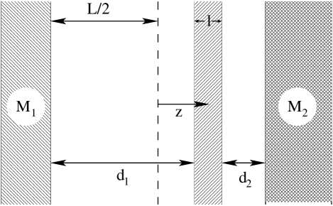
FIG. 2.: A dielectric slab in a planar cavity shown schematically. The arrow indicates the direction of the force on the slab.

This gives

$$f = \frac{\hbar}{2\pi^{2}}\int_{0}^{\infty}d\xi\int dkk\kappa\times$$ (36)

$$\sum_{q=p,s}\left[\frac{r(r_{2}e^{2i\beta d_{2}}-r_{1}e^{2i\beta d_{1}})}{N}\right]^{q}_{\omega=i\xi},$$

$$N =1-r(r_{1}e^{2i\beta d_{1}}+r_{2}e^{2i\beta d_{2}})$$ (38)

$$+d(r^{2}-t^{2})r_{1}r_{2}e^{2i\beta(d_{1}+d_{2})},$$

where the expression in the brackets is to be calculated for $q$-polarization. Using Eqs. (48) and (52), $r$ and $t$ can be further expressed entirely in terms of the reflection coefficient for the cavity-slab interface $\rho=(1-\eta)/(1+\eta)$ [where $\eta^{p}=\varepsilon\beta_{s}/\varepsilon_{s}\beta$ and $\eta^{s}=\beta_{s}/\beta$] as

$$r=\rho\frac{1-e^{2i\beta_{s}l}}{1-\rho^{2}e^{2i\beta_{s}l}},\;\;\;t=\frac{(1-\rho^{2})e^{i\beta_{s}l}}{1-\rho^{2}e^{2i\beta_{s}l}}.$$ (39)

Note that for a perfectly conducting ($\varepsilon_{s}\rightarrow\infty$) slab, we have $r^{p}=-r^{s}=1$ and $t^{q}=0$.

The force $f$, as given by Eq. (38), may be positive or negative, depending on the dielectric properties of the slab and cavity mirrors as well as on the position of the slab. One may easily verify that this equation gives the correct result for the force on a perfectly conducting plate in an empty cavity with ideally reflecting walls. Indeed, since in this case $t^{2}=0$, N factorizes and Eq. (38) splits to ($r^{2}=rr_{1}=rr_{2}=r_{1}r_{2}=1$)

$$f=f_{-}(d_{2})-f_{-}(d_{1}),$$ (40)

where

$$f_{-}(d) = \frac{\hbar}{\pi^{2}}\int_{0}^{\infty}d\xi\int_{0}^{\infty}dkk\frac{\kappa}{e^{2\kappa d}-1}$$ (41)

$$= \frac{\hbar}{3\pi^{2}c^{3}}\int_{0}^{\infty}d\xi\xi\frac{\frac{d}{d\xi}\left[\sqrt{\varepsilon(i\xi)}\xi\right]^{3}}{e^{2\sqrt{\varepsilon(i\xi)}\xi d/c}-1}$$ (42)

is the force on the left mirror of a dispersive ideal cavity [cf. Eqs. (3) and (20), with the index $j$ dropped]. The second line here is obtained upon a partial integration over $\xi$ and upon calculating the $\xi$-derivative of the integral over $k$ (see Ref. [32]). For the empty cavity [$\varepsilon(i\xi)=1$], the integrals in Eq. (42) become elementary giving the well-known result

$$f=\frac{\pi^{2}\hbar c}{240}\left(\frac{1}{d^{4}_{2}}-\frac{1}{d^{4}_{1}}\right),$$ (43)

according to which the plate is attracted to the closer cavity mirror. For a partially transmitting plate, the vacuum-field fluctuations in regions (1) and (2) of the cavity are no longer independent of each other and considerable deviations from the above simple result may occur especially for realistic cavity mirrors. Clearly, in this case, in order to explore the combined effect of the nearby walls on a planar (nano)object, one must analyze Eq. (38) numerically.

IV Summary

Using the properties of the macroscopic field operators appropriate for dissipative systems and a convenient Green function for a multilayer, in this work we have obtained general results for the Casimir force and energy applicable to local layered absorbing systems. We have also established a relationship between the Casimir force (and energy) in two different layers and, as an application of the theory, calculated the Casimir force on a dielectric slab in a realistic planar cavity.

Green function

Denoting the (conserved) wave vector parallel to the system surfaces by ${\bf k}=(k_{x},k_{y})$, we write the wave vector of an rightward (leftward) propagating wave in an $l$th layer as ${\bf K}^{\pm}_{l}={\bf k}\pm\beta_{l}\hat{\bf z}$, where

$$\beta_{l}=\sqrt{\tilde{k}^{2}_{l}-k^{2}}=\beta_{l}^{\prime}+i\beta_{l}^{\prime\prime},\;\;\;\beta_{l}^{\prime}\geq 0,\;\;\beta_{l}^{\prime\prime}\geq 0.$$ (44)

With this notation, the Green function dyadic for the scattered field in the $j$th layer reads [29]

$$\tensor{\bf G}^{\rm sc}_{j}({\bf r},{\bf r}^{\prime};\omega)=\frac{i}{2\pi}\int\frac{d^{2}{\bf k}}{\beta_{j}}e^{i{\bf k}\cdot({\bf r}_{\parallel}-{\bf r}_{\parallel}^{\prime})}\sum_{q=p,s}\frac{e^{i\beta_{j}d_{j}}}{D_{qj}}\xi_{q}\times$$ (45)

$$\left\{r^{q}_{j-}e^{i\beta_{j}z_{-}}\hat{\bf e}^{+}_{qj}({\bf k})\left[\hat{\bf e}^{+}_{qj}(-{\bf k})e^{-i\beta_{j}z^{\prime}_{+}}+r^{q}_{j+}\hat{\bf e}^{-}_{qj}(-{\bf k})e^{i\beta_{j}z^{\prime}_{+}}\right]\right.$$ (46)

$$\left.+r^{q}_{j+}e^{i\beta_{j}z_{+}}\hat{\bf e}^{-}_{qj}({\bf k})\left[\hat{\bf e}^{-}_{qj}(-{\bf k})e^{-i\beta_{j}z^{\prime}_{-}}+r^{q}_{j-}\hat{\bf e}^{+}_{qj}(-{\bf k})e^{i\beta_{j}z^{\prime}_{-}}\right]\right\},$$ (47)

$\displaystyle D_{qj}=1-r^{q}_{j-}r^{q}_{j+}e^{2i\beta_{j}d_{j}},\;\;\;\xi_{p}=1,\;\;\xi_{s}=-1,$

$\displaystyle z_{-}\equiv z,\;\;z_{+}\equiv d_{j}-z,\;\;0\leq z\leq d_{j},$

$$\hat{\bf e}^{\mp}_{pj}({\bf k})=\frac{1}{\tilde{k}_{j}}(\pm\beta_{j}\hat{\bf k}+k\hat{\bf z}),\;\;\;\hat{\bf e}^{\mp}_{sj}({\bf k})=\hat{\bf k}\times\hat{\bf z}\equiv\hat{\bf n},$$ (48)

where $r^{q}_{j\pm}\equiv r^{q}_{j/n(0)}$ are, respectively, the transmission and reflection coefficient of the upper (lower) stack of layers bounding the layer $(j)$. Clearly, for the outmost layers, $l=n\;(0)$, we have $r^{q}_{n+}=0$ and $r^{q}_{0-}=0$. Also, one must let $d_{n}\;(d_{0})=0$ since these quantities appear only formally. The remaining Fresnel coefficients satisfy

$$r^{q}_{i/j/k}=r^{q}_{i/j}+\frac{t^{q}_{i/j}t^{q}_{j/i}r^{q}_{j/k}e^{2i\beta_{j}d_{j}}}{1-r^{q}_{j/i}r^{q}_{j/k}e^{2i\beta_{j}d_{j}}},$$ (50)

$$t^{q}_{i/j/k}=\frac{t^{q}_{i/j}t^{q}_{j/k}e^{i\beta_{j}d_{j}}}{1-r^{q}_{j/i}r^{q}_{j/k}e^{2i\beta_{j}d_{j}}}=\frac{\beta_{i}}{\beta_{k}}t^{q}_{k/j/i},$$ (51)

and, for a single $i-j$ interface, reduce to

$$r^{q}_{ij}=\frac{\beta_{i}-\gamma^{q}_{ij}\beta_{j}}{\beta_{i}+\gamma^{q}_{ij}\beta_{j}},\;\;\;t^{q}_{ij}=\sqrt{\gamma^{q}_{ij}}(1+r^{q}_{ij}),$$ (52)

where $\gamma^{p}_{ij}=\varepsilon_{i}/\varepsilon_{j}$ and $\gamma^{s}_{ij}=1$, respectively.

Performing the derivations indicated in Eq.  (14) and using

$${\bf K}^{\pm}_{j}({\bf k})\times\hat{\bf e}^{\pm}_{qj}({\bf k})=\tilde{k_{j}}\xi_{q}\hat{\bf e}^{\pm}_{q^{\prime}j}({\bf k}),\;\;\;p^{\prime}=s,\;\;s^{\prime}=p,$$ (53)

we find that $\tensor{\bf G}^{B,\rm sc}_{j}({\bf r},{\bf r}^{\prime};\omega)$ is given by Eq. (A2) multiplied by $-\tilde{k}_{j}^{2}$ and with $\hat{\bf e}^{\pm}_{qj}\rightarrow\hat{\bf e}^{\pm}_{q^{\prime}j}$. Noting that the equal-point Green function dyadics consist only of diagonal elements, we easily find

$$\tensor{\bf G}_{j}^{\rm sc}({\bf r},{\bf r};\omega)=\frac{i}{2\pi\tilde{k}_{j}^{2}}\int\frac{d^{2}{\bf k}}{\beta_{j}}\times$$ (54)

$$\left\{\hat{\bf k}\hat{\bf k}\frac{\beta_{j}^{2}}{D_{pj}}\left[2r^{p}_{j-}r^{p}_{j+}e^{2i\beta_{j}d_{j}}-r^{p}_{j-}e^{2i\beta z_{-}}-r^{p}_{j+}e^{2i\beta z_{+}}\right]\right.$$ (55)

$$+\hat{\bf n}\hat{\bf n}\frac{\tilde{k}_{j}^{2}}{D_{sj}}\left[2r^{s}_{j-}r^{s}_{j+}e^{2i\beta_{j}d_{j}}+r^{s}_{j-}e^{2i\beta_{j}z_{-}}+r^{s}_{j+}e^{2i\beta_{j}z_{+}}\right]$$ (56)

$$\left.+\hat{\bf z}\hat{\bf z}\frac{k^{2}}{D_{pj}}\left[2r^{p}_{j-}r^{p}_{j+}e^{2i\beta_{j}d_{j}}+r^{p}_{j-}e^{2i\beta_{j}z_{-}}+r^{p}_{j+}e^{2i\beta_{j}z_{+}}\right]\right\},$$ (57)

and $\tensor{\bf G}^{B,\rm sc}_{j}({\bf r},{\bf r};\omega)$ is given by this equation multiplied by $\tilde{k}_{j}^{2}$ and with $p\leftrightarrow s$. The traces $G^{\rm sc}_{j,\parallel}({\bf r},{\bf r};\omega)$ and $G^{B,\rm sc}_{j,\parallel}({\bf r},{\bf r};\omega)$ can be easily recognized from these equations and one has, for example,

$$\tilde{k}_{j}^{2}\left[G^{\rm sc}_{j,\parallel}({\bf r},{\bf r};\omega)-G^{\rm sc}_{j,zz}({\bf r},{\bf r};\omega)\right]=\frac{i}{2\pi}\int\frac{d^{2}{\bf k}}{\beta_{j}}\times$$ (58)

$$\left\{\frac{\beta_{j}^{2}}{D_{pj}}\left[2r^{p}_{j-}r^{p}_{j+}e^{2i\beta_{j}d_{j}}-r^{p}_{j-}e^{2i\beta z_{-}}-r^{p}_{j+}e^{2i\beta z_{+}}\right]\right.$$ (59)

$$+\frac{\tilde{k}_{j}^{2}}{D_{sj}}\left[2r^{s}_{j-}r^{s}_{j+}e^{2i\beta_{j}d_{j}}+r^{s}_{j-}e^{2i\beta_{j}z_{-}}+r^{s}_{j+}e^{2i\beta_{j}z_{+}}\right]$$ (60)

$$\left.-\frac{k^{2}}{D_{pj}}\left[2r^{p}_{j-}r^{p}_{j+}e^{2i\beta_{j}d_{j}}+r^{p}_{j-}e^{2i\beta_{j}z_{-}}+r^{p}_{j+}e^{2i\beta_{j}z_{+}}\right]\right\},$$ (61)

while $G^{B,\rm sc}_{j,\parallel}({\bf r},{\bf r};\omega)-G^{B,\rm sc}_{j,zz}({\bf r},{\bf r};\omega)$ is given by this equation with $p\leftrightarrow s$. Adding these two quantities, one finds that the curly bracket in Eq.  (17) is equal to

$$\{\ldots\} = -8\pi i\int\frac{d^{2}{\bf k}}{(2\pi)^{2}}\beta_{j}\times$$ (63)

$$\left[\frac{r^{p}_{j-}r^{p}_{j+}e^{2i\beta_{j}d_{j}}}{D_{pj}}+\frac{r^{s}_{j-}r^{s}_{j+}e^{2i\beta_{j}d_{j}}}{D_{sj}}\right].$$

REFERENCES

• [1] H. B. G. Casimir, Porc. K. Ned. Akad. Wet. 51, 793 (1948).
• [2] E. M. Lifshitz, Zh. Eksp. Teor. Fiz. 29, 94 (1995) [Sov. Phys. JETP 2, 73 (1956)].
• [3] J. Schwinger, L. L. DeRaad, Jr., and K. A. Milton, Ann. Phys. (N. Y.) 115, 1 (1978).
• [4] P. W. Milonni, The Quantum Vacuum. An Introduction to Quantum Electrodynamics (San Diego, Academic, 1994) Chap. 7.
• [5] For new developments in the Casimir effect and an extensive list of references see M. Bordag, U. Mohideen, G. L. Klimchitskaya, and V. M. Mostepanenko, Phys. Rep. 353, 1 (2002).
• [6] S. K. Lamoreaux, Phys. Rev. Lett. 78, 5 (1997); ibid 81, 5475(E) (1998).
• [7] U. Mohideen nad A. Roy, Phys. Rev. Lett. 81, 4549 (1998).
• [8] G. Bressi, G. Carugno, R. Onofrio, and G. Ruoso, Phys. Rev. Lett. 88, 041804 (2002)
• [9] S. K. Lamoreaux, Phys. Rev. A 59, R3149 (1999).
• [10] A. Lambrecht, and S. Reynaud, Phys. Rev. Lett. 84, 5672 (2000).
• [11] N. G. van Kampen, B. R. A. Nijboer, and K. Schram, Phys. Lett. 26A, 307, (1968).
• [12] K. Schram, Phys. Lett. 43A, 283, (1973).
• [13] F. Zhou and L. Spruch, Phys. Rev. A 52, 297 (1995).
• [14] G. L. Klimchitskaya, U. Mohideen, and V. M. Mostepanenko, Phys. Rev. A 61, 062107 (2000).
• [15] L. S. Brown and G. J. Maclay, Phys. Rev. 184, 1272 (1969).
• [16] L. D. Landau and E. M. Lifshitz, Electrodynamics of Continuous Media, (Pergamon, Oxford, 1991). Chap. 9.
• [17] See, e.g., I. Brevik and G. Einvoll, Phys. Rev. D 37, 2977 (1988).
• [18] D. Kupiszewska, Phys. Rev. A 46, 2286 (1992).
• [19] D. Kupiszewska nad J. Mostowski, Phys. Rev. A 41, 4636 (1990).
• [20] M. T. Jaekel and S. Reynaud, J. Phys. I (France), 1, 1395 (1991); A. Lambrecht, M. T. Jaekel, and S. Reynaud, Phys. Lett. A 225, 188 (1997).
• [21] R. Mathloob, A. Keshavarz, and D. Sedighi, Phys. Rev. A 60, 3410 (1999).
• [22] R. Esquivel-Sirvent, C. Villarreal, and G. H. Cocoletzi, Phys. Rev. A 64, 052108 (2001).
• [23] R. Esquivel-Sirvent, C. Villarreal, W. L. Mochán, and G. H. Cocoletzi, phys. stat. sol. (b), 230, 409 (2002).
• [24] R. Mathloob, Phys. Rev. 60, 3421 (1999).
• [25] R. Mathloob and H. Falinejad, Phys. Rev. A 64, 042102 (2001).
• [26] W. L. Mochán, C. Villarreal, and R. Esquivel-Sirvent, e-Print arxiv: quant-ph/0206119.
• [27] T. Gruner and D.-G. Welsch, Phys. Rev. A 53, 1818 (1996); H. T. Dung, L. Knöll, and D.-G. Welsch, ibid, 57, 3931 (1998); S. Scheel, L. Knöll, and D.-G. Welsch, ibid, 58, 700 (1998).
• [28] R. Matloob, R. Loudon, S. Barnett, and J. Jeffers, Phys. Rev. A 52, 4823 (1995); R. Matloob and R. Loudon, ibid 53, 4567 (1996); R. Matloob, ibid 60, 50 (1999).
• [29] M. S.Tomaš, Phys. Rev. A 51, 2545 (1995).
• [30] J. D. Jackson, Classical Electrodynamics, 2nd ed. (Willey, New York, 1975) Chap. 6.
• [31] E. M. Lifshitz and L. P. Pitaevskii, Statistical Physics, Part 2, (Pergamon Press, Oxford, 1991) Ch 8.
• [32] M. Schaden, L. Spruch and F. Zhou, Phys. Rev. A 57, 1108 (1998).