Continuous variable teleportation of a quantum state onto a macroscopic body

Abstract

We study the possibility to teleport an unkown quantum state onto the vibrational degree of freedom of a movable mirror. The quantum channel between the two parties is established by exploiting radiation pressure effects.

I Introduction

Quantum state teleportation is undoubtedly one of the most fascinating developments of quantum information processing [1].

Teleportation of an unknown quantum state is its immaterial transport through a classical channel employing one of the most puzzling resources of Quantum Mechanics: entanglement [2]. A variety of possible experimental schemes have been proposed and few of them partially realized in the discrete variable case involving the polarization state of single photons[3, 4, 5]. A successful achievement has been then obtained in the continuous variable case of an optical field [6]. However, the tantalizing problem of extending quantum teleportation at the macroscopic scale still remains open.

Recently, in the perspective of demonstrating and manipulating the quantum properties of bigger and bigger objects [7], it has been shown [8] how it is possible to entangle two massive macroscopic oscillators, like movable mirrors, by using radiation pressure effects. The creation of such an entanglement at the macroscopic level suggests an avenue for achieving teleportation of a continuous variable state of a radiation field onto the vibrational state of a mirror.

II The Model

We consider the situation where an unknown quantum state of a radiation field is prepared by a verifier (Victor) and sent to an analyzing station (Alice). Here we shall provide a protocol which enables Alice to teleport the unknown quantum state of the radiation onto a collective vibrational degree of freedom of a macroscopic, perfectly reflecting, mirror placed at a remote station (Bob) (see Fig. 1). For simplicity we consider only the motion and the elastic deformations of the mirror taking place along the spatial direction $x$, orthogonal to its reflecting surface. Then we consider an intense laser beam impinging on the surface of the mirror, whose radiation pressure realizes an optomechanical coupling [9]. In fact, the electromagnetic field exerts a force on the mirror proportional to its intensity and, at the same time, it is phase-shifted by the mirror displacement from the equilibrium position [10]. In the limit of small mirror displacements, and in the interaction picture with respect to the free Hamiltonian of the electromagnetic field and the mirror displacement field ${\hat{x}({\bf r},t)}$ (${\bf r}$ is the coordinate on the mirror surface), one has the following Hamiltonian [11]

$${\hat{H}} = -\int\,d^{2}{\bf r}\,{\hat{P}}({\bf r},t){\hat{x}}({\bf r},t)\,,$$ (1)

where ${\hat{P}({\bf r},t)}$ is the radiation pressure force [9]. All the continuum of electromagnetic modes with positive longitudinal wave vector $q$, transverse wave vector ${\bf k}$, and frequency $\omega=\sqrt{c^{2}(k^{2}+q^{2})}$ ($c$ being the light speed in the vacuum) contributes to the radiation pressure force. We are adopting the interaction picture with respect to the free Hamiltonian of the electromagnetic field of the continuum and of the field of elastic deformations of the mirror. Following Ref.[9], and considering linearly polarized radiation with the electric field parallel to the mirror surface, we have

$${\hat{P}}({\bf r},t) = -\frac{\hbar}{8\pi^{3}}\int d{\bf k}\int dq\int d{\bf k^{\prime}}\int dq^{\prime}\frac{c^{2}qq^{\prime}}{\sqrt{\omega\omega^{\prime}}}({\bf u}_{k}\cdot{\bf u}_{k^{\prime}}){\bf u}_{q}$$ (2)

$$\times \left\{{\hat{a}}({\bf k},q){\hat{a}}({\bf k}^{\prime},q^{\prime})\exp[-i(\omega+\omega^{\prime})t+i({\bf k}+{\bf k}^{\prime})\cdot{\bf r}]\right.$$ (6)

$$\left.+{\hat{a}}^{{\dagger}}({\bf k},q){\hat{a}}^{{\dagger}}({\bf k}^{\prime},q^{\prime})\exp[i(\omega+\omega^{\prime})t-i({\bf k}+{\bf k}^{\prime})\cdot{\bf r}]\right.$$

$$\left.+{\hat{a}}({\bf k},q){\hat{a}}^{{\dagger}}({\bf k}^{\prime},q^{\prime})\exp[-i(\omega-\omega^{\prime})t+i({\bf k}-{\bf k}^{\prime})\cdot{\bf r}]\right.$$

$$\left.+{\hat{a}}^{{\dagger}}({\bf k},q){\hat{a}}({\bf k}^{\prime},q^{\prime})\exp[i(\omega-\omega^{\prime})t-i({\bf k}-{\bf k}^{\prime})\cdot{\bf r}]\right\}\,,$$

where ${\hat{a}}({\bf k},q)$ are the continuous mode destruction operators having transverse wave vector ${\bf k}$ and positive longitudinal wave vector component $q$, obeying the commutation relations

$$\left[{\hat{a}}({\bf k},q),{\hat{a}}({\bf k}^{\prime},q^{\prime})\right]=\delta({\bf k}-{\bf k}^{\prime})\delta(q-q^{\prime})\,.$$ (7)

Furthermore, the electromagnetic wave frequencies $\omega$ and $\omega^{\prime}$ are given by $\omega^{2}=c^{2}(k^{2}+q^{2})$ and $\omega^{\prime 2}=c^{2}(k^{\prime 2}+q^{\prime 2})$, and ${\bf u}_{k}$, ${\bf u}_{q}$ denote dimensionless unit vectors parallel to ${\bf k}$, $q$ respectively.

The mirror displacement ${\hat{x}({\bf r},t)}$ is generally given by a superposition of many acoustic modes [11]; however, a single vibrational mode description can be adopted whenever detection is limited to a frequency bandwidth including a single mechanical resonance. In particular, focused light beams are able to excite Gaussian acoustic modes, in which only a small portion of the mirror, localized at its center, vibrates. These modes have a small waist $w$, a large mechanical quality factor $Q$, a small effective mass $M$ [11], and the simplest choice is to choose the fundamental Gaussian mode with frequency $\Omega$, i.e.,

$${\hat{x}}({\bf r},t)=\sqrt{\frac{\hbar}{2M\Omega}}\left[{\hat{b}}e^{-i\Omega t}+{\hat{b}}^{{\dagger}}e^{i\Omega t}\right]\exp(-r^{2}/w^{2})\,.$$ (8)

By inserting Eqs.(6) and (8) in Eq.(1) and integrating over the variable ${\bf r}$ one obtains

$${\hat{H}} = -\frac{\hbar w^{2}}{8\pi^{2}}\sqrt{\frac{\hbar}{2M\Omega}}\int d{\bf k}\int dq\int d{\bf k^{\prime}}\int dq^{\prime}\frac{c^{2}qq^{\prime}}{\sqrt{\omega\omega^{\prime}}}({\bf u}_{k}\cdot{\bf u}_{k^{\prime}}){\bf u}_{q}$$ (9)

$$\times \left\{{\hat{a}}({\bf k},q){\hat{a}}({\bf k}^{\prime},q^{\prime})\exp[-i(\omega+\omega^{\prime})t-({\bf k}+{\bf k}^{\prime})^{2}w^{2}/4]\right.$$ (13)

$$\left.+{\hat{a}}^{{\dagger}}({\bf k},q){\hat{a}}^{{\dagger}}({\bf k}^{\prime},q^{\prime})\exp[i(\omega+\omega^{\prime})t-({\bf k}+{\bf k}^{\prime})^{2}w^{2}/4]\right.$$

$$\left.+{\hat{a}}({\bf k},q){\hat{a}}^{{\dagger}}({\bf k}^{\prime},q^{\prime})\exp[-i(\omega-\omega^{\prime})t-({\bf k}-{\bf k}^{\prime})^{2}w^{2}/4]\right.$$

$$\left.+{\hat{a}}^{{\dagger}}({\bf k},q){\hat{a}}({\bf k}^{\prime},q^{\prime})\exp[i(\omega-\omega^{\prime})t-({\bf k}-{\bf k}^{\prime})^{2}w^{2}/4]\right\}\times\left\{{\hat{b}}e^{-i\Omega t}+{\hat{b}}^{{\dagger}}e^{i\Omega t}\right\}\,.$$

In common situations, the acoustical waist $w$ is much larger than typical optical wavelengths [11], and therefore we can approximate $\exp\left\{-({\bf k}\pm{\bf k^{\prime}})^{2}w^{2}/4\right\}w^{2}/4\pi\simeq\delta({\bf k}\pm{\bf k^{\prime}})$ and then integrate Eq. (13) over ${\bf k^{\prime}}$, obtaining

$${\hat{H}} = -\frac{\hbar}{2\pi}\sqrt{\frac{\hbar}{2M\Omega}}\int d{\bf k}\int dq\int dq^{\prime}\frac{c^{2}qq^{\prime}}{\sqrt{\omega\omega^{\prime}}}$$ (14)

$$\times \left\{-{\hat{a}}({\bf k},q){\hat{a}}(-{\bf k},q^{\prime})\exp[-i(\omega+\omega^{\prime})t]\right.$$ (18)

$$\left.-{\hat{a}}^{{\dagger}}({\bf k},q){\hat{a}}^{{\dagger}}(-{\bf k},q^{\prime})\exp[i(\omega+\omega^{\prime})t]\right.$$

$$\left.+{\hat{a}}({\bf k},q){\hat{a}}^{{\dagger}}({\bf k},q^{\prime})\exp[-i(\omega-\omega^{\prime})t]\right.$$

$$\left.+{\hat{a}}^{{\dagger}}({\bf k},q){\hat{a}}({\bf k},q^{\prime})\exp[i(\omega-\omega^{\prime})t]\right\}\times\left\{{\hat{b}}e^{-i\Omega t}+{\hat{b}}^{{\dagger}}e^{i\Omega t}\right\}\,.$$

We now make the Rotating Wave Approximation (RWA), that is, we neglect all the terms oscillating in time faster than the mechanical frequency $\Omega$. This means averaging the Hamiltonian over a time $\tau$ such that $\Omega\tau\gg 1$, yielding the following replacements in Eq. (18)

$$\exp\left\{\pm i(\omega^{\prime}\pm\omega\pm\Omega)t\right\}\rightarrow\frac{2\pi}{\tau}\delta(\omega^{\prime}\pm\omega\pm\Omega).$$ (19)

The parameter $\tau$ is not arbitrary, but its inverse, $1/\tau=\Delta\nu_{det}$, is the detection bandwidth, that is, the spectral resolution of the detection apparata used at Alice station.

Since $\omega$ and $\omega^{\prime}$ are positive and $\Omega$ is much smaller than typical optical frequencies, the two terms $\delta(\omega^{\prime}+\omega\pm\Omega)$ give no contribution, while the other two terms can be rewritten as

$$\frac{2\pi}{\tau}\delta(\omega^{\prime}-\omega\pm\Omega)=2\pi\Delta\nu_{det}\delta(q^{\prime}-\bar{q}_{\pm})\frac{\omega^{\prime}(\bar{q}_{\pm})}{c^{2}\bar{q}_{\pm}},$$ (20)

where $\bar{q}_{\pm}=\sqrt{(\omega\pm\Omega)^{2}/c^{2}-k^{2}}$. Integrating over $q^{\prime}$ we get

$${\hat{H}} = -\hbar\Delta\nu_{det}\sqrt{\frac{\hbar}{2M\Omega}}\int d{\bf k}\int dq\frac{q}{\sqrt{\omega}}\left\{{\hat{a}}({\bf k},q){\hat{a}}^{{\dagger}}\left({\bf k},\bar{q}_{+}\right){\hat{b}}\;\sqrt{\omega+\Omega}+{\hat{a}}({\bf k},q){\hat{a}}^{{\dagger}}\left({\bf k},\bar{q}_{-}\right){\hat{b}}^{{\dagger}}\sqrt{\omega-\Omega}\right.$$ (22)

$$\left.+{\hat{a}}^{{\dagger}}({\bf k},q){\hat{a}}\left({\bf k},\bar{q}_{+}\right){\hat{b}}^{{\dagger}}\sqrt{\omega+\Omega}+{\hat{a}}^{{\dagger}}({\bf k},q){\hat{a}}\left({\bf k},\bar{q}_{-}\right){\hat{b}}\sqrt{\omega-\Omega}\right\}\,,$$

where we have used the fact that $\omega^{\prime}(\bar{q}_{\pm})=\omega\pm\Omega$.

We now consider the situation where the radiation field incident on the mirror is characterized by an intense, quasi-monochromatic, laser field with trasversal wave vector ${\bf k_{0}}$, longitudinal wave vector $q_{0}$, cross-sectional area $A$, and power ${\wp}$. Since this component is very intense, it can be treated as classical and one can approximate ${\hat{a}}({\bf k},q)\simeq\alpha({\bf k},q)$ in Eq. (22), where (with an appropriate choice of phases)

$$\alpha({\bf k},q)=-i\sqrt{\frac{(2\pi)^{3}{\wp}}{\hbar\omega_{0}cA}}\delta({\bf k}-{\bf k_{0}})\delta(q-q_{0})\,,$$ (23)

with $\omega_{0}=c\sqrt{{\bf k_{0}}^{2}+q_{0}^{2}}$.

Due to the Dirac delta, the only nonvanishing terms in the optomechanical interaction driven by the intense laser beam involve only two back-scattered waves, that is, the sidebands of the driving beam at frequencies $\omega_{0}\pm\Omega$, as described by

$${\hat{H}} = i\hbar\Delta\nu_{det}\sqrt{\frac{\hbar}{2M\Omega}}q_{0}\sqrt{\frac{{\wp}}{\hbar\omega_{0}cA}}\left\{\sqrt{\frac{\omega_{0}+\Omega}{\omega_{0}}}{\hat{a}}^{{\dagger}}\left({\bf k_{0}},\bar{q}_{+}\right){\hat{b}}+\sqrt{\frac{\omega_{0}-\Omega}{\omega_{0}}}{\hat{a}}^{{\dagger}}\left({\bf k_{0}},\bar{q}_{-}\right){\hat{b}}^{\dagger}\right.$$ (25)

$$\left.-\sqrt{\frac{\omega_{0}+\Omega}{\omega_{0}}}{\hat{a}}\left({\bf k_{0}},\bar{q}_{+}\right){\hat{b}}^{\dagger}-\sqrt{\frac{\omega_{0}-\Omega}{\omega_{0}}}{\hat{a}}\left({\bf k_{0}},\bar{q}_{-}\right){\hat{b}}\right\},$$

where now $\bar{q}_{\pm}=\sqrt{(\omega_{0}\pm\Omega)^{2}/c^{2}-k_{0}^{2}}$. The physical process described by this interation Hamiltonian is very similar to a stimulated Brillouin scattering [12], even though in this case the Stokes and anti-Stokes component are back-scattered by the acoustic waves at reflection, and the optomechanical coupling is provided by the radiation pressure and not by the dielectric properties of the mirror.

In practice, either the driving laser beam and the back-scattered modes are never monochromatic, but have a nonzero bandwidth. In general the bandwidth of the back-scattered modes is determined by the bandwidth of the driving laser beam and that of the acoustic mode. However, due to its high mechanical quality factor, the spectral width of the mechanical resonance is negligible (about $1$ Hz) and, in practice, the bandwidth of the two sideband modes $\Delta\nu_{mode}$ coincides with that of the incident laser beam. It is then convenient to consider this nonzero bandwidth to redefine the bosonic operators of the Stokes and anti-Stokes modes to make them dimensionless,

$${\hat{a}}_{1} = 2\pi\sqrt{\frac{2\pi\Delta\nu_{mode}}{cA}}{\hat{a}}\left({\bf k_{0}},\bar{q}_{-}\right)=2\pi\sqrt{\frac{\Delta q}{A}}{\hat{a}}\left({\bf k_{0}},\bar{q}_{-}\right)$$ (26)

$${\hat{a}}_{2} = 2\pi\sqrt{\frac{2\pi\Delta\nu_{mode}}{cA}}{\hat{a}}\left({\bf k_{0}},\bar{q}_{+}\right)=2\pi\sqrt{\frac{\Delta q}{A}}{\hat{a}}\left({\bf k_{0}},\bar{q}_{+}\right),$$ (27)

so that Eq.(25) reduces to an effective Hamiltonian

$${\hat{H}}_{eff}=-i\hbar\chi({\hat{a}}_{1}{\hat{b}}-{\hat{a}}^{{\dagger}}_{1}{\hat{b}}^{{\dagger}})-i\hbar\theta({\hat{a}}_{2}{\hat{b}}^{{\dagger}}-{\hat{a}}^{{\dagger}}_{2}{\hat{b}})\,,$$ (28)

where the couplings $\chi$ and $\theta$ are given by

$$\chi = q_{0}\Delta\nu_{det}\sqrt{\frac{\hbar}{2M\Omega}}\sqrt{\frac{{\wp}}{\Delta\nu_{mode}\hbar\omega_{0}}}\sqrt{\frac{\omega_{0}-\Omega}{\omega_{0}}}=\cos\phi_{0}\sqrt{\frac{{\wp}\Delta\nu_{det}^{2}(\omega_{0}-\Omega)}{2M\Omega c^{2}\Delta\nu_{mode}}}$$ (29)

$$\theta = \chi\sqrt{\frac{\omega_{0}+\Omega}{\omega_{0}-\Omega}},$$ (30)

with $\phi_{0}=\arccos(cq_{0}/\omega_{0})$, is the angle of incidence of the driving beam. It is possible to verify that with the above definitions, the Stokes and anti-Stokes annihilation operators $a_{1}$ and $a_{2}$ satisfy the usual commutation relations $\left[a_{i},a_{j}^{\dagger}\right]=\delta_{i,j}$.

III System dynamics

Eq. (28) contains two interaction terms: the first one, between modes ${\hat{a}}_{1}$ and ${\hat{b}}$, is a parametric-type interaction leading to squeezing in phase space [13], and it is able to generate the EPR-like entangled state which has been used in the continuous variable teleportation experiment of Ref. [6]. The second interaction term, between modes ${\hat{a}}_{2}$ and ${\hat{b}}$, is a beam-splitter-type interaction [13], which may degrade the entanglement between modes ${\hat{a}}_{1}$ and ${\hat{b}}$ generated by the first term.

The Hamiltonian (28) leads to a system of linear Heisenberg equations, namely

$$\dot{\hat{a}}_{1} = \chi{\hat{b}}^{{\dagger}}\,,$$ (32)

$$\dot{\hat{b}} = \chi{\hat{a}}_{1}^{{\dagger}}-\theta{\hat{a}}_{2}\,,$$ (33)

$$\dot{\hat{a}}_{2} = \theta{\hat{b}}\,.$$ (34)

The solutions read

$${\hat{a}}_{1}(t) = \frac{1}{\Theta^{2}}\left[\theta^{2}-\chi^{2}\cos\left(\Theta t\right)\right]{\hat{a}}_{1}(0)+\frac{\chi}{\Theta}\sin\left(\Theta t\right){\hat{b}}^{{\dagger}}(0)-\frac{1}{\Theta^{2}}\left[\chi\theta-\chi\theta\cos\left(\Theta t\right)\right]{\hat{a}}_{2}^{{\dagger}}(0)\,,$$ (36)

$${\hat{b}}(t) = -\frac{\chi}{\Theta}\sin\left(\Theta t\right){\hat{a}}_{1}^{{\dagger}}(0)+\cos\left(\Theta t\right){\hat{b}}(0)-\frac{\theta}{\Theta}\sin\left(\Theta t\right){\hat{a}}_{2}(0)\,,$$ (37)

$${\hat{a}}_{2}(t) = \frac{1}{\Theta^{2}}\left[\chi\theta-\chi\theta\cos\left(\Theta t\right)\right]{\hat{a}}_{1}^{{\dagger}}(0)-\frac{\theta}{\Theta}\sin\left(\Theta t\right){\hat{b}}(0)-\frac{1}{\Theta^{2}}\left[\chi^{2}-\theta^{2}\cos\left(\Theta t\right)\right]{\hat{a}}_{2}(0)\,,$$ (38)

where $\Theta=\sqrt{\theta^{2}-\chi^{2}}$.

On the other hand, the system dynamics can be easily studied also through the (normally ordered) characteristic function $\Phi(\mu,\nu,\zeta)$, where $\mu,\nu,\zeta$ are the complex variables corresponding to the operators ${\hat{a}}_{1},{\hat{b}},{\hat{a}}_{2}$ respectively. From the Hamiltonian (28) the dynamical equation for $\Phi$ results

$${\dot{\Phi}} = \chi\left(\mu\nu+\mu^{*}\nu^{*}-\mu^{*}\frac{\partial}{\partial\nu}-\mu\frac{\partial}{\partial\nu^{*}}-\nu^{*}\frac{\partial}{\partial\mu}-\nu\frac{\partial}{\partial\mu^{*}}\right)\Phi$$ (40)

$$+\theta\left(\zeta^{*}\frac{\partial}{\partial\nu^{*}}+\zeta\frac{\partial}{\partial\nu}-\nu^{*}\frac{\partial}{\partial\zeta^{*}}-\nu\frac{\partial}{\partial\zeta}\right)\Phi\,,$$

with the initial condition

$$\Phi(t=0)=\exp\left[-\overline{n}|\nu|^{2}\right]\,,$$ (41)

corresponding to the vacuum for the modes ${\hat{a}}_{1}$, ${\hat{a}}_{2}$ and to a thermal state for the mode ${\hat{b}}$. The latter is characterized by an average number of excitations $\overline{n}=[\coth(\hbar\Omega/2k_{B}T)-1]/2$, $T$ being the equilibrium temperature and $k_{B}$ the Boltzmann constant. Then, equation (40) has a Gaussian solution of the form

$$\Phi=\exp\left[-{\cal A}|\mu|^{2}-{\cal B}|\nu|^{2}-{\cal E}|\zeta|^{2}+{\cal C}\mu\nu+{\cal C}\mu^{*}\nu^{*}+{\cal F}\mu\zeta+{\cal F}\mu^{*}\zeta^{*}+{\cal D}\nu\zeta^{*}+{\cal D}\nu^{*}\zeta\right]\,,$$ (42)

where

$${\cal A}(t) = \frac{\chi^{4}}{2\Theta^{4}}\left[\cos\left(2\Theta t\right)-1\right]-2\frac{\chi^{2}\theta^{2}}{\Theta^{4}}\left[\cos\left(\Theta t\right)-1\right]+\overline{n}\frac{\chi^{2}}{2\Theta^{2}}\left[1-\cos\left(2\Theta t\right)\right]\,,$$ (44)

$${\cal B}(t) = \frac{\chi^{2}}{2\Theta^{2}}\left[1-\cos\left(2\Theta t\right)\right]+\frac{\overline{n}}{2}\left[1+\cos\left(2\Theta t\right)\right]\,,$$ (45)

$${\cal C}(t) = -\frac{\chi^{3}}{2\Theta^{3}}\sin\left(2\Theta t\right)+\frac{\chi\theta^{2}}{\Theta^{3}}\sin\left(\Theta t\right)+\overline{n}\frac{\chi}{2\Theta}\sin\left(2\Theta t\right)\,,$$ (46)

$${\cal D}(t) = \frac{\chi^{2}\theta}{2\Theta^{3}}\sin\left(2\Theta t\right)-\frac{\chi^{2}\theta}{\Theta^{3}}\sin\left(\Theta t\right)-\overline{n}\frac{\theta}{2\Theta}\sin\left(2\Theta t\right)\,,$$ (47)

$${\cal E}(t) = \frac{\chi^{2}\theta^{2}}{2\Theta^{4}}\left[\cos\left(2\Theta t\right)-1\right]-2\frac{\chi^{2}\theta^{2}}{\Theta^{4}}\left[\cos\left(\Theta t\right)-1\right]+\overline{n}\frac{\theta^{2}}{2\Theta^{2}}\left[1-\cos\left(2\Theta t\right)\right]\,,$$ (48)

$${\cal F}(t) = \frac{\chi^{3}\theta}{2\Theta^{4}}\left[\cos\left(2\Theta t\right)-1\right]-\frac{\chi\theta}{\Theta^{4}}\left(\chi^{2}+\theta^{2}\right)\left[\cos\left(\Theta t\right)-1\right]+\overline{n}\frac{\chi\theta}{2\Theta^{2}}\left[1-\cos\left(2\Theta t\right)\right]\,.$$ (49)

After an interaction time $t$, the state of the whole system can be expressed in terms of the normally ordered characteristic function as

$${\hat{\rho}}_{1b2}=\int\frac{d^{2}\mu}{\pi}\int\frac{d^{2}\nu}{\pi}\int\frac{d^{2}\zeta}{\pi}\Phi(\mu,\nu,\zeta,t)e^{-|\mu|^{2}-|\nu|^{2}-|\zeta|^{2}}{\hat{D}}_{1}(-\mu){\hat{D}}_{b}(-\nu){\hat{D}}_{2}(-\zeta)\,,$$ (50)

where ${\hat{D}}$ indicates normally ordered displacement operator.

IV Teleportation protocol

The idea is to find an experimentally feasible, modified version of the standard protocol for the teleportation of continuous quantum variables [14, 15], able to minimize the disturbing effects of the beam-splitter-type term in Eq. (28).

First of all, the driving mode is filtered out after reflection on the mirror (see Fig.1), allowing only the modes ${\hat{a}}_{1}$ and ${\hat{a}}_{2}$ to reach Alice’s station. Then Alice performs a heterodyne measurement [16] on the mode ${\hat{a}}_{2}$, projecting it onto a coherent state $|\alpha\rangle$. Alice and Bob are left with an entangled state for the optical Stokes mode $a_{1}$ and the vibrational mode $b$, conditioned to this measurement result, i.e.,

$${\hat{\rho}}_{1b}=N\int\frac{d^{2}\mu}{\pi}\int\frac{d^{2}\nu}{\pi}\int\frac{d^{2}\zeta}{\pi}\Phi(\mu,\nu,\zeta,t)e^{-|\mu|^{2}-|\nu|^{2}-|\zeta|^{2}}{\hat{D}}_{1}(-\mu){\hat{D}}_{b}(-\nu)\langle\alpha|{\hat{D}}_{2}(-\zeta)|\alpha\rangle\,,$$ (51)

and the normalization constant is $N=({\cal E}+1)\exp\left[|\alpha|^{2}/({\cal E}+1)\right]$. Denoting with ${\tilde{\Phi}}(\mu,\nu)$ the normally ordered characteristic function associate to the state (51), we have

$${\tilde{\Phi}}(\mu,\nu) = N\int\frac{d^{2}\zeta}{\pi}\Phi(\mu,\nu,\zeta)e^{-\zeta\alpha^{*}+\zeta^{*}\alpha-|\zeta|^{2}}$$ (52)

$$= \exp\left[-\left({\cal A}-\frac{{\cal F}^{2}}{{\cal E}+1}\right)|\mu|^{2}-\left({\cal B}-\frac{{\cal D}^{2}}{{\cal E}+1}\right)|\nu|^{2}\right.$$ (54)

$$\left.+\left({\cal C}+\frac{\cal FD}{{\cal E}+1}\right)\left(\mu\nu+\mu^{*}\nu^{*}\right)+\frac{\cal F}{{\cal E}+1}\left(\alpha\mu-\alpha^{*}\mu^{*}\right)+\frac{\cal D}{{\cal E}+1}\left(\alpha\nu^{*}-\alpha^{*}\nu\right)\right]\,.$$

Introducing the quadratures

$${\hat{X}}_{a_{1}} = \frac{{\hat{a}}_{1}+{\hat{a}}_{1}^{{\dagger}}}{\sqrt{2}}\,,\quad{\hat{P}}_{{\hat{a}}_{1}}=\frac{{\hat{a}}_{1}-{\hat{a}}_{1}^{{\dagger}}}{i\sqrt{2}}\,,$$ (56)

$${\hat{X}}_{b} = \frac{{\hat{b}}+{\hat{b}}^{{\dagger}}}{\sqrt{2}}\,,\quad{\hat{P}}_{b}=\frac{{\hat{b}}-{\hat{b}}^{{\dagger}}}{i\sqrt{2}}\,.$$ (57)

it is possible to evaluate their correlations through Eq.(52). In particular, defining ${\hat{\bf v}}=({\hat{X}}_{a_{1}},{\hat{P}}_{a_{1}},{\hat{X}}_{b},{\hat{P}}_{b})$, the correlation matrix $\Gamma_{i,j}=\langle{\hat{\bf v}}_{i}{\hat{\bf v}}_{j}+{\hat{\bf v}}_{j}{\hat{\bf v}}_{i}\rangle/2$ results

$$\Gamma=\left(\begin{array}[]{cccc}{\cal A}-\frac{{\cal F}^{2}}{{\cal E}+1}+\frac{1}{2}&0&{\cal C}+\frac{\cal FD}{{\cal E}+1}&0\\ 0&{\cal A}-\frac{{\cal F}^{2}}{{\cal E}+1}+\frac{1}{2}&0&-{\cal C}-\frac{\cal FD}{{\cal E}+1}\\ {\cal C}+\frac{\cal FD}{{\cal E}+1}&0&{\cal B}-\frac{{\cal D}^{2}}{{\cal E}+1}+\frac{1}{2}&0\\ 0&-{\cal C}-\frac{\cal FD}{{\cal E}+1}&0&{\cal B}-\frac{{\cal D}^{2}}{{\cal E}+1}+\frac{1}{2}\end{array}\right)\,.$$ (58)

We now employ the standard protocol for the teleportation of continuous quantum variables [14, 15]. The quantum channel between Alice and Bob is established via two-mode entangled state described by the correlation matrix (58).

An input Gaussian state at Alice’s side can be fully described by its $2\times 2$ covariance matrix $\Gamma^{in}$. Then, the output Gaussain state at Bob’s side would be characterized by the covariance matrix $\Gamma^{out}$. The input-output relation for these matrices can be found as follows. In terms of normally ordered characteristic functions we have

$$\exp\left[-\frac{1}{4}{\bf u}\Gamma^{out}{\bf u}^{T}\right]=\tilde{K}({\bf u})\exp\left[-\frac{1}{4}{\bf u}\Gamma^{in}{\bf u}^{T}\right]$$ (59)

where ${\bf u}=(q,p)$ is the variable vector of the characteristic functions. Instead $\tilde{K}$ is the Fourier transform of the kernel in the integral transform mapping the Wigner function of the input state into the Wigner function of the output state (see e.g. Ref.[17]). In terms of the Wigner function $W_{AB}$ of the state shared by Alice and Bob, it results

$$\tilde{K}({\bf u}) = \int dx_{A}dp_{A}dx_{B}dp_{B}\;e^{-ix_{A}q-ix_{B}q+ip_{A}p-ip_{B}p}\;W_{AB}(x_{A},p_{A},x_{B},p_{B})$$ (60)

$$= \exp\left[-\frac{1}{4}\left(q,-p,q,p\right)\Gamma\left(q,-p,q,p\right)^{T}\right]\,.$$ (61)

Then, it is easy to derive the relations

$$\Gamma_{11}^{out} = \Gamma_{11}^{in}+\left(\Gamma_{11}+2\Gamma_{13}+\Gamma_{33}\right)\,,$$ (63)

$$\Gamma_{12}^{out} = \Gamma_{12}^{in}+\left(\Gamma_{14}-\Gamma_{12}+\Gamma_{34}-\Gamma_{23}\right)\,,$$ (64)

$$\Gamma_{22}^{out} = \Gamma_{22}^{in}+\left(\Gamma_{22}-2\Gamma_{24}+\Gamma_{44}\right)\,.$$ (65)

Thus, the fidelity of the teleportation protocol can be written, with the help of Eqs.(58) and (IV) as

$$F=\frac{1}{1+\left[1+{\cal A}(t)+{\cal B}(t)+2{\cal C}(t)-({\cal F}-{\cal D})^{2}/({\cal E}+1)\right]}\,,$$ (66)

where we have specialized to the case of an input coherent state. In such a case, the upper bound for the fidelity achievable with only classical means and no quantum resources is $F=1/2$ [18].

The fidelity (66) does not depend on the Bob’s local operations. In fact these are merely displacements based on the Alice’s measurement results $X_{+},P_{-},\alpha$, i.e. ${\hat{X}}_{b}\to{\hat{X}}_{b}+\sqrt{2}X_{+}+\sqrt{2}{\rm Re}\{\alpha\}({\cal F}-{\cal D})/({\cal E}+1)$, ${\hat{P}}_{b}\to{\hat{P}}_{b}-\sqrt{2}P_{-}+\sqrt{2}{\rm Im}\{\alpha\}({\cal F}+{\cal D})/({\cal E}+1)$. Note that the amount proportional to ${\cal F}/({\cal E}+1)$ deserves to account for the shifted results $X_{+},P_{-}$ obtained by Alice by virtue of the heterodyne detection (see Eq. (52)), while the amount proportional to ${\cal D}/({\cal E}+1)$ deserves to cancel the diplacement on the ${\hat{b}}$ mode caused again by the heterodyne detection (see Eq. (52)).

To actuate the phase-space displacement, Bob can use again the radiation pressure force. In fact, if the mirror is shined by a bichromatic intense laser field with frequencies $\varpi_{0}$ and $\varpi_{0}+\Omega$, employing again Eq. (1) and the RWA, one is left with an effective interaction Hamiltonian

$$H_{act}\propto{\hat{b}}e^{-i\varphi}+{\hat{b}}^{{\dagger}}e^{i\varphi},$$ (67)

where $\varphi$ is the relative phase between the two frequency components. Any phase space displacement of the mirror vibrational mode can be realized by adjusting this relative phase and the intensity of the laser beam.

Finally, for what concerns the experimental verification of teleportation, that is, the measurement of the final state of the acoustic mode, one can consider a second, intense “reading” laser pulse, and exploit again the optomechanical interaction given by Eq. (28), where now $a_{1}$ and $a_{2}$ are meter modes. It is in fact possible to perform a heterodyne measurement [16] of an appropriate combination of the two back-scattered modes, ${\hat{Z}}={\hat{a}}_{1}-{\hat{a}}_{2}^{{\dagger}}$, if the driving laser beam at frequency $\omega_{0}$ is used as local oscillator and the resulting photocurrent is mixed with a signal oscillating at the frequency $\Omega$. The behaviour of $Z(t)$ as a function of the time duration of the second “measuring” driving beam can be derived from Eqs. (III), that is

$${\hat{Z}}(t)\equiv{\hat{a}}_{1}(t)-{\hat{a}}_{2}^{{\dagger}}(t) = \frac{1}{\Theta}\left[\chi+\theta\right]\sin(\Theta t){\hat{b}}^{{\dagger}}(0)$$ (68)

$$+ \frac{1}{\Theta^{2}}\left[\theta^{2}-\chi^{2}\cos(\Theta t)-\chi\theta+\chi\theta\cos(\Theta t)\right]{\hat{a}}_{1}(0)$$ (69)

$$- \frac{1}{\Theta^{2}}\left[\chi\theta+\chi\theta\cos(\Theta t)-\chi^{2}-\theta^{2}\cos(\Theta t)\right]{\hat{a}}_{2}^{{\dagger}}(0)\,.$$ (70)

It is easy to see that for $\cos(\Theta t)=0$ and $\Theta(\theta+\chi)\gg\theta(\theta-\chi)$ the measured quantity practically coincides with the mode oscillation operator $b^{{\dagger}}(0)$, thus revealing information on the state of the mechanical oscillator.

V Results and Conclusions

Fig. 2 shows the fidelity (66) as a function of the (rescaled) interaction time $t$ for different values of the initial mean thermal phonon number of the mirror acoustic mode $\overline{n}$. The fidelity $F$ is periodic in the interaction time $t$ (see Methods), and we show only one of all possible time windows where $F$ reaches its maximum. The remarkable result shown in Fig. 2 is that this maximum value, $F_{max}\simeq 0.85$, is well above the classical bound $F=0.5$ and that it is surprisingly independent of the initial temperature of the acoustic mode. This is apparently in contrast with previous results [19] showing that entanglement is no longer useful above one thermal photon (or phonon). This effect could be ascribed to quantum interference phenomena, and opens the way for the demonstration of quantum teleportation of states of macroscopic systems. However, thermal noise has still important effects so that, in practice, any experimental implementation needs an acoustic mode cooled at low temperatures (see however Refs. [20, 22] for effective cooling mechanism of acoustic modes). In fact, we see from Fig. 2 that by increasing $\overline{n}$, the useful time interval becomes narrower. That means the necessity of designing precise driving laser pulses in order to have a well defined interaction time. Furthermore, the time interval within which the classical communication from Alice to Bob, and the phase space displacement by Bob have to be made, becomes shorter and shorter with increasing temperature, because the vibrational state projected by Alice’s Bell measurement heats up in a time of the order of $(\gamma_{m}\overline{n})^{-1}$, where $\gamma_{m}$ is the mechanical damping constant. The effects of mechanical damping can be instead neglected during the back-scattering process stimulated by the intense laser beam. In fact, mechanical damping rates of about $\gamma_{m}\simeq 1$ Hz are available, and therefore negligible with respect to the typical values of the coupling constants $\chi\simeq\theta\simeq 5\times 10^{5}$ Hz, and $\Theta\simeq 10^{3}$ Hz, determining the Hamiltonian dynamics (see Methods). Such values are obtained with the following choice of parameters: ${\wp}=10$W, $\omega_{0}\sim 2\times 10^{15}$ Hz, $\Omega\sim 5\times 10^{8}$ Hz, $\Delta\nu_{det}\sim 10^{7}$ Hz, $\Delta\nu_{mode}\sim t^{-1}\sim 10^{3}$ Hz, and $M\sim 10^{-10}$ Kg, which are those used in Fig. 2. These parameters are slightly different from those of already performed optomechanical experiments [21, 22]. However, using a thinner silica crystal and considering higher frequency modes, the parameters we choose could be obtained. These choices show the difficulties one meets in trying to extend genuine quantum effects as teleportation into the macroscopic domain.

The continuous variable teleportation protocol presented here modifies the standard one of Refs. [14, 15] by adding a heterodyne measurement on the “spectator” mode ${\hat{a}}_{2}$. This additional measurement performed by Alice is important because it significantly improves the teleportation protocol. In fact, it is easy to see that if no measurement is performed on the anti-Stokes mode, the resulting fidelity for the teleportation of coherent states is always smaller with respect to that with the heterodyne measurement. In particular, there is still a maximum value of the fidelity, $F_{max}=0.80$ in this case, independent of temperature, but the useful interaction time interval becomes much narrower for increasing temperature.

It is worth remarking that the present teleportation scheme provides also a very powerful cooling mechanism for the acoustic mode. As matter of fact, its effective number of thermal excitations soon after the two homodyne measurements at Alice station becomes $\overline{n}_{eff}=1+{\cal A}+{\cal B}+2{\cal C}-({\cal F}-{\cal D})^{2}/({\cal E}+1)$. It reduces to $\overline{n}+1$ in absence of entanglement, where $1$ represents the noise introduced by the protocol. Instead, the optomechanical interaction for a proper time permits to achieve $\overline{n}_{eff}=0.17$, i.e., an $80\%$ reduction of thermal noise at once, at the moment of Alice’s measurement, thanks to the entanglement. To this end, the classical communication and the phase space displacement at Bob’s site are unnecessary, since they do not affect the state variances.

In conclusion, we have proposed a simple scheme to teleport an unknown quantum state of a radiation field onto a macroscopic, collective vibrational degree of freedom of a massive mirror. The basic resource of entanglement is attained by means of the optomechanical coupling provided by the radiation pressure. Here we have shown the teleportation of the quantum information contained in an unknown quantum state of a radiation field to a collective degree of freedom of a massive object. This scheme could be easily extended in principle to realize a transfer of quantum information between two massive objects. In fact Victor could use tomographic reconstruction schemes, again based on the ponderomotive interaction (see [23]), to “read” the quantum state of a vibrational mode of another mirror and use this information to prepare the state of the radiation field to be sent to Alice. The present result could be challenging tested with present technology, and opens new perspectives towards the use of quantum mechanics in macroscopic world. For example, we recognize possible technological applications such as the preparation of nonclassical states of micro-electro-mechanical systems (MEMS) [24], where the oscillation frequency could be higher and, consequently, the working temperature can be raised.

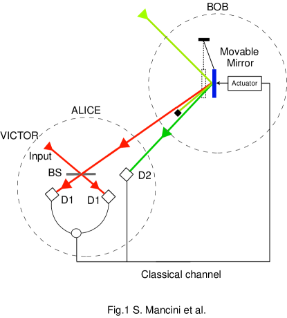
FIG. 1.: Schematic description of the system. A laser field at frequency $\omega_{0}$ impinges on the mirror oscillating at frequency $\Omega$. In the reflected field two sideband modes are excited at frequencies $\omega_{1}=\omega_{0}-\Omega$ and $\omega_{2}=\omega_{0}+\Omega$. These two modes then reach Alice’s station. The mode at frequency $\omega_{2}$ is subjected to a heterodyne measurement $D2$, while the mode at frequency $\omega_{1}$ is mixed in the 50-50 beam splitter BS with the unknown input given by Victor. A Bell-like measurement $D1$ is then performed on this combination and the result, combined with the heterodyne one, is fed-forward to Bob as two bits of classical information. Finally, he actuates the displacement in the phase space of the moving mirror.

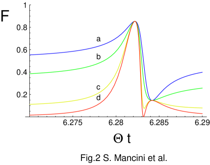
FIG. 2.: Fidelity $F$ vs the scaled time $\Theta t$. Curves a, b, c, d are for $\overline{n}=0$, 1, 10, $10^{3}$, respectively. The values of parameters are: $\wp=10$ W; $\Omega=5\times 10^{8}$ Hz; $\Delta\nu_{det}=10^{7}$ Hz; $M=10^{-10}$ Kg; $\omega_{0}=2\times 10^{15}$ Hz, $\Delta\nu_{mode}=10^{3}$ Hz.

REFERENCES

• [1] C. H. Bennett, et al., Phys. Rev. Lett. 70, 1895 (1993).
• [2] A. Einstein, B. Podolsky and N. Rosen, Phys Rev. 47, 777 (1935).
• [3] D. Bouwmeester, et al., Nature (London) 390, 575 (1997).
• [4] D. Boschi, et al., Phys. Rev. Lett. 80, 1121 (1998).
• [5] T. Jennewein, et al., Phys. Rev. Lett. 88, 017903 (2002).
• [6] A. Furusawa, et al. Science 282, 706 (1998).
• [7] B. Julsgaard, A. Kozhekin and E. S. Polzik, Nature (London) 413, 400 (2001).
• [8] S. Mancini, V. Giovannetti, D. Vitali and P. Tombesi, Phys. Rev. Lett. 88, 120401 (2002).
• [9] P. Samphire, R. Loudon, and M. Babiker, Phys. Rev. A 51, 2726 (1995).
• [10] C. K. Law, Phys. Rev. A 51, 2537 (1995).
• [11] M. Pinard, et al., Eur. Phys. J. D 7, 107 (1999).
• [12] J. Perina, Quantum Statistics of Linear and Nonlinear Optical Phenomena, (Reidel, Dordrecht, 1984).
• [13] D. F. Walls and G. J. Milburn, Quantum Optics, (Springer, Berlin, 1994).
• [14] L. Vaidman, Phys. Rev. A 49, 1473 (1994).
• [15] S. L. Braunstein and H. J. Kimble, Phys. Rev. Lett. 80, 869 (1998).
• [16] H. P. Yuen and J. H. Shapiro, IEEE Trans. Info. Theory IT-26, 78 (1980).
• [17] A. V. Chizhov, L. Knöll and D. G. Welsch, Phys. Rev. A 65, 022310 (2002).
• [18] S. L. Braunstein, C. A. Fuchs, H. J. Kimble and P. van Loock, Phys. Rev. A 64, 022321 (2001).
• [19] L. M. Duan, G. Giedke, J. I. Cirac and P. Zoller, Phys. Rev. Lett. 84, 2722 (2000).
• [20] D. Vitali, S. Mancini, L. Ribichini and P. Tombesi, Phys. Rev. A 65, 063803 (2002).
• [21] I. Tittonen, et al., Phys. Rev. A 59, 1038 (1999).
• [22] P. F. Cohadon, A. Heidmann and M. Pinard, Phys. Rev. Lett. 83, 3174 (1999).
• [23] S. Mancini and P. Tombesi, in Coherence and Quantum Optics VII, edited by J. H. Eberly and E. Wolf, (Plenum, New York, 1996), p. 607.
• [24] A. N. Cleland and M. L. Roukes, Nature (London) 392, 160 (1998).
Refer to caption