Quantum Fluctuations in Josephson Junction Comparators

Abstract

We have developed a method for calculation of quantum fluctuation effects, in particular of the uncertainty zone developing at the potential curvature sign inversion, for a damped harmonic oscillator with arbitrary time dependence of frequency and for arbitrary temperature, within the Caldeira-Leggett model. The method has been applied to the calculation of the gray zone width $\Delta I_{x}$ of Josephson-junction balanced comparators driven by a specially designed low-impedance RSFQ circuit. The calculated temperature dependence of $\Delta I_{x}$ in the range 1.5 to 4.2K is in a virtually perfect agreement with experimental data for Nb-trilayer comparators with critical current densities of 1.0 and 5.5 kA/cm², without any fitting parameters.

The current attention to quantum information processing (see, e.g., the recent monograph Nielsen and Chuang (2000)) has renewed interest in fast ”single-shot” quantum measurements, especially in potentially scalable solid-state systems. Among such systems, superconductor ”balanced comparator”, based on two similar Josephson junctions (Fig. 1a), stands apart as a very simple, scalable system for which quantum-limited sensitivity has already been demonstrated experimentally Semenov et al. (1997).

The device is essentially a SQUID (see, e.g., Likharev (1986)) in which two similar junctions are biased in series by a source of Josephson phase difference $\phi_{e}(t)$, and in parallel by the current $I_{x}$ to be measured. Let the system with $\left|\phi_{e}\right|<\pi$ settle in an equilibrium state $\phi=\phi_{i}$, and then apply a rapid phase change $\Delta\phi_{e}=2\pi$. (This can be readily done using the so-called RSFQ circuitry - see, e.g., the recent review Bunyk et al. (2000).) As a result, the system becomes statically unstable and the Josephson phase $\phi$ has to switch to one of adjacent stable states, depending on the sign of $I_{x}$. (For junctions with substantial damping, the choice is limited by two states closest to the initial value of $\phi$: $\phi_{f}=\phi_{i}\pm\pi$).

This process may be readily understood using the ”magnetic language”: the driver circuit providing the pulse $\Delta\phi_{e}=2\pi$ in fact injects a single flux quantum into a superconducting loop formed by its output stage and the comparator (Fig. 1a). Since the loop is low-inductive (non-quantizing), the flux quantum has to drop out across one of the comparator junctions, depending on the sign of $I_{x}$. This transient process produces a large (discrete) output signal, the so-called SFQ pulse $V(t)$ with $\int V(t)dt=\Phi_{0}=h/2e$ across the corresponding junction. Such a pulse may be readily picked up and registered by relatively crude devices Bunyk et al. (2000), so that the accuracy of the $I_{x}$ sign measurement is defined entirely by the comparator.

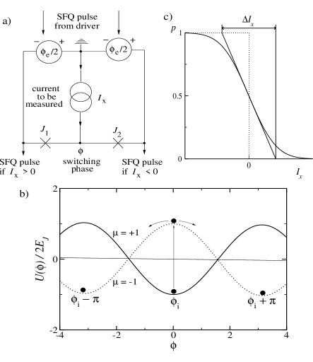
Figure 1: (a) The balanced comparator, (b) its potential energy profile $U(\phi)$ for $I_{x}=0.01I_{c}$ and two values of the external phase $\phi_{e}$ ($\mu=\cos(\phi_{e}/2)$), and (c) probability $p$ of comparator switching into state $\phi_{f}=\phi_{i}-\pi$ as a function of the measured current $I_{x}$ (schematically).

In the absence of fluctuations, the boundary between the two possible outcomes would be infinitely sharp - see the dashed line in Fig. 1c; however, fluctuations create a finite ”gray zone” of $I_{x}$ where probability $p$ of switching to a certain finite state changes gradually from 0 to 1 - see the solid line in Fig. 1c. The gray zone width, which is traditionally defined as

$$\Delta I_{x}\equiv\left|\frac{dp}{dI_{x}}\right|_{I_{x}=0}^{-1},$$ (1)

characterizes the accuracy of the single-shot measurement. This width, including its temperature dependence, has been measured in several special experiments with externally-shunted Josephson junctions Filippov et al. (1995); Semenov et al. (1997). However, theoretically it has been only calculated Filippov (1995, 1996) for a special function $\phi_{e}(t)$ enabling an analytical solution of the problem, but rather different from that used in experiments. Thus, the comparison of theory and experiments was not completely conclusive. The goal of this work has been to develop a general method of calculation of $\Delta I_{x}$ for an arbitrary waveform $\phi_{e}(t)$ and to compare the results with experimental data Filippov et al. (1995); Semenov et al. (1997).

The potential energy of the balanced comparator (Fig. 1a) may be presented in the form

$$U(\phi)=-2E_{J}\cos\left[\frac{\phi_{e}(t)}{2}\right]\cos\phi-\frac{\hbar}{2e}I_{x}\phi,$$ (2)

where $E_{J}\equiv\hbar I_{c}/2e$ is the Josephson coupling energy scale, and $I_{c}$ is the critical current of a single junction. (In the simplest case, neither $\phi_{e}(t)$ nor $I_{x}$ depend on the state of the comparator.) Notice that the part of ”washboard” potential profile, contributed by the Josephson junctions, changes sign when $\phi_{e}(t)$ is increased beyond $\pi$. This is exactly the reason of the system switching to one of the newly stable states $\phi_{f}\approx\phi_{i}\pm\pi$ (Fig. 1b). Now let $\left|I_{x}\right|$ and the natural current scales of thermal and quantum fluctuations, $I_{T}=(2e/\hbar)T$ and $I_{Q}=(2e/\hbar)\hbar\omega_{p}=2e\omega_{p}$, respectively (where $\omega_{p}$ is the plasma frequency Likharev (1986)), all be much smaller than $I_{c}$, and the potential inversion time be of the order of, or shorter than the characteristic time of system dynamics. Then the choice of the final state is determined by the system evolution close to the point $\phi=0$. In order to describe this evolution, we may keep only two leading, linear and quadratic, terms in the Taylor expansion of the potential energy (2) near this point:

$$\frac{U(\phi)}{2E_{J}}=\frac{\mu(t)\phi^{2}}{2}-\frac{I_{x}}{2I_{c}}\phi+\mbox{const},\;\;\mu(t)\equiv\cos\frac{\phi_{e}(t)}{2}.$$ (3)

This means that the state choice problem in the original, nonlinear system is reduced to that of a damped time-dependent harmonic oscillator with frequency $\omega(t)$ defined as $\omega^{2}(t)=\mu(t)\omega_{p}^{2}$, where $\mu$ is switched rapidly from a positive initial value $\mu_{i}$ (in experiments Filippov et al. (1995); Semenov et al. (1997), close to 1) to a negative final value $\mu_{f}=-\mu_{i}$.

The probability of switching to a final state with $\phi_{f}<\phi_{i}$ may be found as

$$p=\lim_{t\rightarrow\infty}\int\limits_{-\infty}^{\phi_{max}(t)}\rho(\phi,\phi,t)\,d\phi,$$ (4)

where $\rho(\phi,\phi^{\prime},t)$ is the system’s density matrix traced over the degrees of freedom of the environment, and $\phi_{max}(t)$ is the coordinate of the maximum of potential (3) after inversion. Converting to coordinates $\eta\equiv\phi+\phi^{\prime}$ and $\xi\equiv\phi-\phi^{\prime}$, we can express $\rho(\phi,\phi,t)=(1/2)\rho(\eta,0,t)$ via the system propagator $J(\eta,\xi,t|\eta_{i},\xi_{i},0)$:

$$\rho(\eta,0,t)=\iint\limits_{-\infty}^{+\infty}J(\eta,0,t|\eta_{i},\xi_{i},0)\rho(\eta_{i},\xi_{i},0)\,d\eta_{i}\,d\xi_{i}.$$ (5)

To find the propagator, we may use the Caldeira-Leggett approach Caldeira and Leggett (1983) with the linear distribution of the environment oscillators, which gives a quantitatively correct description of systems with externally shunted Josephson junctions. According to this theory,

$$J(\eta,\xi,t|\eta_{i},\xi_{i},0)=\iint\exp\left[\frac{iS(\eta,\xi)-\theta(\eta,\xi)}{\hbar}\right]D\eta D\xi,$$ (6)

$$S(\eta,\xi)=\int\limits_{0}^{t}\mathcal{L}(\eta,\xi)d\tau-\left.\frac{M\gamma}{2}\eta\xi\right|_{0}^{t},$$ (7)

$$\begin{split}\theta(\eta,\xi)=&\frac{2M\gamma}{\pi}\int\limits_{0}^{\Omega}d\omega\omega\coth(\frac{\hbar\omega}{2T})\\ &\times\int\limits_{0}^{t}d\tau\int\limits_{0}^{\tau}ds\xi(\tau)\xi(s)\cos[\omega(\tau-s)].\end{split}$$ (8)

Here, $\mathcal{L}=M(\dot{\phi})^{2}/2-M\mu(t)\omega_{p}^{2}\phi^{2}/2$ is the Lagrangian of the mechanical oscillator equivalent to our system, with mass $M=2E_{p}/\omega_{p}^{2}$, while $\gamma=\omega_{p}^{2}/2\omega_{c}$ is its damping parameter, where $\omega_{c}\equiv(2e/\hbar)I_{c}R$, and $R$ is the shunting resistance Likharev (1986). Parameter $\Omega$ is the cutoff frequency of the environment oscillators. To evaluate the path integral (6), we represent coordinates $\eta,\xi$ as a sum of the path parts $\eta(\tau),\xi(\tau)$ minimizing the action $S$, and small fluctuations $\tilde{\eta},\tilde{\xi}$. The path parts satisfy the following equations Caldeira and Leggett (1983):

$$\omega_{p}^{-2}\frac{d^{2}\eta}{d\tau^{2}}+\omega_{c}^{-1}\frac{d\eta}{d\tau}+\mu(\tau)\eta=I_{x}/I_{c},$$ (9)

$$\omega_{p}^{-2}\frac{d^{2}\xi}{d\tau^{2}}-\omega_{c}^{-1}\frac{d\xi}{d\tau}+\mu(\tau)\xi=0.$$ (10)

It is convenient to present solutions of these equations as follows:

$$\eta(\tau,t) = \eta_{i}a_{1}(\tau,t)+\eta a_{2}(\tau,t)+(I_{x}/I_{c})a(\tau,t),$$ (11)

$$\xi(\tau,t) = \xi_{i}b_{1}(\tau,t)+\xi b_{2}(\tau,t),$$ (12)

where functions $a_{1,2}$ and $b_{1,2}$ as functions of $\tau$ obey the uniform versions of equations (9), (10) with the following boundary conditions: $a_{1}(0)=b_{1}(0)=1$, $a_{1}(t)=b_{1}(t)=0$, $a_{2}(0)=b_{2}(0)=0$, $a_{2}(t)=b_{2}(t)=1$, while $a$ is the solution to Eq. (9) with the unit right-hand part and boundary conditions $a(0)=a(t)=0$.

Plugging all these expressions into Eq. (6), and carrying out a lengthy but straightforward (Gaussian) integration, we get

$$J(\eta,\xi,t|\eta_{i},\xi_{i},0)=F^{2}(t)\exp\left\{i\left[K_{1}\eta_{i}\xi_{i}+K_{2}\eta\xi-L\eta_{i}\xi-N\eta\xi_{i}+\frac{I_{x}}{I_{c}}(Q_{1}\xi_{i}+Q_{2}\xi)\right]-[A\xi^{2}+B\xi\xi_{i}+C\xi_{i}^{2}]\right\},$$ (13)

$$\begin{aligned} \left(\begin{array}[]{c}K_{1}\\ K_{2}\end{array}\right)&=\frac{E_{J}}{\hbar}\int\limits_{0}^{t}d\tau\left\{\frac{1}{\omega_{p}^{2}}\left(\begin{array}[]{c}a^{\prime}_{1}b^{\prime}_{1}\\ a^{\prime}_{2}b^{\prime}_{2}\end{array}\right)-\mu(\tau)\left(\begin{array}[]{c}a_{1}b_{1}\\ a_{2}b_{2}\end{array}\right)+\frac{1}{2\omega_{c}}\left(\begin{array}[]{c}a_{1}b^{\prime}_{1}-a_{1}^{\prime}b_{1}\\ a_{2}b^{\prime}_{2}-a_{2}^{\prime}b_{2}\end{array}\right)\right\}+\frac{E_{J}}{2\hbar\omega_{c}}\left(\begin{array}[]{c}1\\ -1\end{array}\right),\\ \left(\begin{array}[]{c}N\\ L\end{array}\right)&=-\frac{E_{J}}{\hbar}\int\limits_{0}^{t}d\tau\left\{\frac{1}{\omega_{p}^{2}}\left(\begin{array}[]{c}a^{\prime}_{2}b^{\prime}_{1}\\ a^{\prime}_{1}b^{\prime}_{2}\end{array}\right)-\mu(\tau)\left(\begin{array}[]{c}a_{2}b_{1}\\ a_{1}b_{2}\end{array}\right)+\frac{1}{2\omega_{c}}\left(\begin{array}[]{c}a_{2}b^{\prime}_{1}-a_{2}^{\prime}b_{1}\\ a_{1}b^{\prime}_{2}-a_{1}^{\prime}b_{2}\end{array}\right)\right\},\\ \left(\begin{array}[]{c}Q_{1}\\ Q_{2}\end{array}\right)&=\frac{E_{J}}{\hbar}\int\limits_{0}^{t}d\tau\left\{\frac{1}{\omega_{p}^{2}}\left(\begin{array}[]{c}a^{\prime}b^{\prime}_{1}\\ a^{\prime}b^{\prime}_{2}\end{array}\right)-\mu(\tau)\left(\begin{array}[]{c}ab_{1}\\ ab_{2}\end{array}\right)+\frac{1}{2\omega_{c}}\left(\begin{array}[]{c}ab^{\prime}_{1}-a^{\prime}b_{1}\\ ab^{\prime}_{2}-a^{\prime}b_{2}\end{array}\right)+\left(\begin{array}[]{c}b_{1}\\ b_{2}\end{array}\right)\right\},\\ \left(\begin{array}[]{c}A\\ B\\ C\end{array}\right)&=\frac{E_{J}}{\pi\hbar\omega_{c}}\int\limits_{0}^{\Omega}d\omega\omega\coth\left(\frac{\hbar\omega}{2T}\right)\int\limits_{0}^{t}\int\limits_{0}^{t}d\tau\,ds\cos[\omega(\tau-s)]\left(\begin{array}[]{c}b_{2}(\tau,t)b_{2}(s,t)\\ b_{1}(s,t)b_{2}(\tau,t)+b_{1}(\tau,t)b_{2}(s,t)\\ b_{1}(\tau,t)b_{1}(s,t)\end{array}\right),\end{aligned}$$ (14)

where $F^{2}(t)$ is a normalization factor, and the prime represents differentiation over $\tau$.

These formulas present the generalization of Eq. (6.26) of Ref. Caldeira and Leggett (1983) to the case of arbitrary time dependence of the oscillator potential curviture $\mu(t)$. Equations (5), (13) show that if the initial density matrix is Gaussian (as it is, e.g., for a system in thermal equilibrium), the final matrix is also Gaussian, with the average phase $\langle\phi\rangle$ and variance $\langle\phi^{2}\rangle$ determined by parameters $K_{1},N,Q_{1}$ and $C$. (Other parameters affect only the final phase velocity distribution, which is not important for our particular problem.)

Using the definition (1), the gray zone width may now be calculated as

$$\begin{split}\Delta I_{x}=&\lim_{t\rightarrow\infty}\frac{\left(2\pi\left\langle\phi^{2}\right\rangle\right)^{1/2}}{\left|\frac{d}{dI_{x}}\left\langle\phi\right\rangle\right|}\\ =&2\pi^{1/2}I_{c}\frac{\left[C+4K_{1}^{2}\langle\phi^{2}\rangle_{i}+\left(I_{c}/2e\omega_{c}\right)^{2}\langle\dot{\phi}^{2}\rangle_{i}\right]^{1/2}}{K_{1}\mu_{i}^{-1}+Q_{1}}.\end{split}$$ (15)

This is our central result. For the particular case of the RSFQ driver circuit used in experiments Filippov et al. (1995); Semenov et al. (1997), the function $\mu(t)$ has been calculated numerically from the circuit schematics, using the PSCAN software package Polonsky et al. (1991). Since functions $a(\tau,t)$ and $b(\tau,t)$ are exponential near the boundary points $\tau=0$ and $\tau=t$, the standard ”shooting” methods for the numerical calculation of these functions would be unstable. Because of this we have used the relaxation method Keller (1992). Upon the calculation of $a(\tau,t)$ and $b(\tau,t)$, parameters $K_{1}$ and $Q_{1}$ were obtained by the standard numerical integration using the trapezoidal approximation Press et al. (1997). $C$ was calculated using 3D Monte Carlo integration where an integration by parts helps control the discontinuity at $\omega\rightarrow 0$. Due to the shape of the function $b_{1}$, a combination of stratified and importance sampling greatly increases the convergence time, so a variant of the VEGAS algorithm Press et al. (1997) was used. The bath oscillator cutoff frequency $\Omega$ was taken large enough $(50\omega_{p})$ to avoid any effect on the calculation results.

Figure 2 shows $\mu$ and the essential parameters of the Gaussian distribution as functions of $t$. One can see that if the interval $[0,t]$ includes the time point $t_{inv}$ of the potential curvature sign inversion, with both $t_{inv}$ and $t-t_{inv}$ much longer than the oscillator’s reciprocal bandwidth $\Delta\omega^{-1}\approx\max[1/\omega_{c},\omega_{c}/2\omega_{p}^{2}]$, then $C\gg 1$, and $Q_{1}\gg K_{1}$, so that the final density matrix and switching probability $p$ do not depend on the initial state of the system. In this limit, Eq. (15) takes a very simple form:

$$\Delta I_{x}=2\pi^{1/2}I_{c}\frac{C^{1/2}}{Q_{1}}.$$ (16)

Figure 3 shows the resulting temperature dependence of the gray zone width for several values of the inertia parameter (normalized junction capacitance) $\beta_{c}\equiv(\omega_{c}/\omega_{p})^{2}$. At high temperatures, $\Delta I_{x}$ grows as $T^{1/2}$ due to thermal fluctuations, while at $T\rightarrow 0$ it saturates due to quantum fluctuations. Note also that the dependence of $\Delta I_{x}$ on $\beta_{c}$ is different for high and low temperatures: if thermal fluctuations dominate, the gray zone width depends on $\beta_{c}$ only weakly, saturating at comparable values at both $\beta_{c}\rightarrow 0$ and $\beta_{c}\rightarrow\infty$. However, in the quantum fluctuation range ($T\rightarrow 0$), $\Delta I_{x}$ grows as $\beta_{c}^{1/4}$ at high damping ($\beta_{c}\rightarrow 0$) and saturates in the opposite limit of low damping. All these dependences may be qualitatively understood from the following simple consideration: $\Delta I_{x}$ crudely equals to the signal current that creates the phase shift $\phi=I_{x}/2I_{c}$ equal to the r.m.s. value of phase noise in thermal equilibrium. The latter value may be estimated assuming that an equivalent current noise source Likharev (1986) with equilibrium spectral density $S_{I}(\omega)=(4/R)(\hbar\omega/2)\coth(\hbar\omega/2T)$ acts on a time-independent linear oscillator within the bandwidth $\Delta\omega$ defined above.

Figure 4 shows the comparison of our results with experimental data for comparators based on niobium-trilayer (Nb/AlO_x/Nb) Josephson junctions with $I_{c}\mid_{T=4.2K}$ = 145 $\mu A$, $\beta_{c}=1$, for two values of the critical current density: $j_{c}$ = 1 kA/cm² Filippov et al. (1995) and 5.5 kA/cm² Semenov et al. (1997). One can see that besides the deviation of the two lowest-$T$ points in experiments Filippov et al. (1995), which was apparently caused by sample self-heating, the theory gives a virtually perfect description of experimental results, without any fitting parameters. (The possibility of a substantial external noise contribution to $\Delta I_{x}$ in experiments Filippov et al. (1995); Semenov et al. (1997) has been ruled out by special control experiments using similar comparators, fabricated on the same chip, but driven by ”softer” waveforms.)

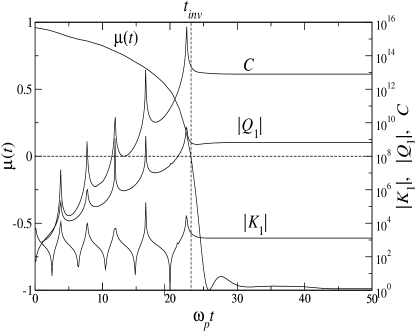
Figure 2: Calculated function $\mu(t)$ and parameters of the final phase distribution for the RSFQ drivers used in experiments Filippov et al. (1995); Semenov et al. (1997) for $\beta_{c}=1$. The time scale $\omega_{p}^{-1}$ is close to 1.1 ps for the critical current density $j_{c}$ = 1 kA/cm² Filippov et al. (1995) and 0.47 ps for $j_{c}$ = 5.5 kA/cm² Semenov et al. (1997).

Figure 3: Temperature dependence of $\Delta I_{x}$ for $\mu(t)$ shown in Fig. 2, calculated for several values of $\beta_{c}$. Dashed lines represent the thermal limit.

Figure 4: Temperature dependence of $\Delta I_{x}$. Points show experimental data from Refs. Filippov et al. (1995); Semenov et al. (1997). The dashed lines are results of calculation taking into account the Ambegoakar-Baratoff temperature dependence of $I_{c}$. The solid lime is the theory for an instantaneous change of $\mu$ from +1 to -1.

To summarize, we have developed a method of analysis of quantum fluctuations at the inversion of the potential curvature sign of a damped harmonic oscillator. When applied to Josephson junction comparator, these results may be used for numerical caculation of the gray zone width $\Delta I_{x}$. Such calculation for the Nb-trilayer comparators Filippov et al. (1995); Semenov et al. (1997) gave a nearly perfect agreement with experimental data. Our result may be also generalized to the case of a finite inductive impedance of the source of the signal $I_{x}$, which is typical for Josephson junction systems, e.g., magnetic flux qubits Friedman et al. (2000); van der Wal et al. (2000). Indeed, the impedance may be described by connecting the source inductance $L$ in parallel with the source of $I_{x}$ in Fig. 1a. An elementary calculation shows that this leads to re-normalization of function $\mu(t)$:

$$\mu(t)\rightarrow\cos\left[\frac{\phi_{e}(t)}{2}\right]+\frac{1}{2\lambda},\text{ \ \ }\lambda\equiv 2\pi\frac{LI_{c}}{\Phi_{0}}.$$ (17)

This means that if the inductance is not too low, $\lambda>1/2$, the input SFQ pulse $\Delta\phi_{e}=2\pi$ develops an instability of phase $\phi$ just as was described above, and our theory gives a ready recipe for the calculation of $\Delta I_{x}$ and hence of the signal flux resolution $\Delta\Phi_{x}=L\Delta I_{x}$.

However, in order to reduce dephasing, flux qubits typically require unshunted Josephson junctions. This is why a natural next task would be a calculation of $\Delta\Phi_{x}$ for the case when damping is dominated by quasiparticle tunneling in unshunted junctions. For this, the Caldeira-Legget action (7) should be replaced with one found by Ambegaokar $\it{et}$ $\it{al.}$ Ambegaokar et al. (1982).

Useful discussions with D. V. Averin, J. E. Lukens, Yu. A. Polyakov, and V. K. Semenov are gratefully acknowledged. The work was supported in part by DoD, ARDA, and AFOSR as a part of DURINT program.

References

Nielsen and Chuang (2000)
M. A. Nielsen and
I. L. Chuang,
Quantum Computation and Quantum Information
(Cambridge U. Press, Cambridge, UK,
2000).
Semenov et al. (1997)
V. K. Semenov
et al., IEEE Trans. on Appl. Supercond.
7, 3617 (1997).
Likharev (1986)
K. K. Likharev,
Dynamics of Josephson Junctions and Circuits
(Gordon and Breach, New York, 1986).
Bunyk et al. (2000)
P. Bunyk,
K. Likharev, and
D. Zinoviev,
Int. J. of High Speed Electron. and Syst.
11, 257 (2000).
Filippov et al. (1995)
T. V. Filippov
et al., IEEE Trans. on Appl. Supercond.
5, 2240 (1995).
Filippov (1995)
T. V. Filippov,
JETP Letters 61,
858 (1995).
Filippov (1996)
T. V. Filippov,
Russian Microelectronics 25,
250 (1996).
Caldeira and Leggett (1983)
A. O. Caldeira and
A. J. Leggett,
Physica 121 A,
587 (1983).
Polonsky et al. (1991)
S. V. Polonsky,
V. K. Semenov,
and P. N.
Shevchenko, Spercond. Sci. Technol.
4, 667 (1991).
Keller (1992)
H. B. Keller,
Numerical Methods for Two-Point Boundary-Value
Problems (Dover, 1992).
Press et al. (1997)
W. H. Press
et al., Numerical Recipes in C
(Cambridge, 1997).
Friedman et al. (2000)
J. R. Friedman
et al., Nature
406, 43 (2000).
van der Wal et al. (2000)
C. H. van der Wal
et al., Science
290, 773 (2000).
Ambegaokar et al. (1982)
V. Ambegaokar,
U. Eckert, and
G. Schön,
Phys. Rev. Lett. 48,
1745 (1982).