CAN THE GAME
BE QUANTUM?

Abstract

The game in which acts of participants don’t have an adequate description in terms of Boolean logic and classical theory of probabilities is considered. The model of the game interaction is constructed on the basis of a non-distributive orthocomplemented lattice. Mixed strategies of the participants are calculated by the use of probability amplitudes according to the rules of quantum mechanics. A scheme of quantization of the payoff function is proposed and an algorithm for the search of Nash equilibrium is given. It is shown that differently from the classical case in the quantum situation a discrete set of equilibrium is possible.

Introduction

It often occurs that mathematical structures discovered when solving some class of problems find their natural application in totally different areas. The mathematical formalism of quantum mechanics operating with such notions as ”observable”, ”state”, ”probability amplitude” is not an exception to this rule. The goal of the present paper is to show that the language of quantum mechanics, initially applied to the description of the microworld, is adequate for the description of some macroscopic systems and situations where Planck’s constant plays no role. It is natural to look for applications of the formalism of quantum mechanics in those situations when one has interactions with the element of indeterminacy. So in recent papers [5, 6, 7] the connection of quantum mechanics with decision problems in the conditions of the indeterminacy is discussed. In [3] as well as more recently [4] it was shown that the quantum mechanical formalism can be applied to description of macroscopical systems when the distributive property for random events is broken. In the physics of the microworld non-distributivity has an objective status and must be present in principle. For macroscopic systems the non-distributivity of random events expresses some specific case of the observer’s ”ignorance”.

In the present paper a quantum mechanical formalism is applied to the analysis of a conflict interaction, the mathematical model for which is an antagonistic game of two persons. The game is based on a generalisation of examples of the macroscopical automata simulating the behaviour of some quantum systems considered earlier in [1, 2]. A special feature of the game considered is that the players acts go in contradiction with the usual logic. The consequence is breaking of the classical probability interpretation of the mixed strategy: the sum of the probabilities for alternate outcomes may be larger than one. The cause of breaking of the basic property of the probability is in the non-distributivity of the logic. The partners relations are such that the disjunction ”or”, conjunction ”and” and the operation of negation do not form a Boolean algebra but an orthocomplemented non-distributive lattice. However this ortholattice happens to be just that which describes some properties of a quantum system with spin one half. This leads to new ”quantum” rules for the calculations of the average profit and new representation of the mixed strategy, the role of which is played by the ”wave function” – the normalised vector in a finite dimensional Hilbert space. Calculations of probabilities are made according to the standard rules of quantum mechanics. Differently from the examples of quantum games considered in [8, 9, 10] where the ”quantum” nature of the game was conditioned by the microparticles or quantum computers based on them, in our case we deal with a macroscopic game, the quantum nature of which has nothing to do with microparticles. This gives the hope that our example is one of many analogous situations in biology, economics etc where the formalism of quantum mechanics can be used.

1 .  Where were you Bob?

The game ”Wise Alice” formulated in our paper is a modification of the well known game when each of the participants names one of some previously considered objects. In the case if the results differ, one of the players wins from the other some agreed sum of money. The participants of our game A and B, call them Alice and Bob have a quadratic box in which a ball is located. Bob puts his ball in one of the corners of the box but doesn’t tell his partner which corner. Alice must guess in which corner Bob has put his ball. The rules of the game are such that Alice can ask Bob questions supposing the two-valued answer: ”yes” or ”no”. It is supposed that Bob is honest and always tells the truth. In the case of a ”yes” answer Alice is satisfied, in the opposite case she asks Bob to pay her some compensation. However, differently from other such games [11] the rules of this game (see Fig. 1) have one specific feature: Bob has the possibility to move the ball to any of the adjacent vertices of the square after Alice asks her question. This additional condition decisively changes the behaviour of Bob, making him to become active under the influence of Alice’s questions. Due to the fact that negative answers are not profitable for him he, in all possible cases, moves his ball to the convenient adjacent vertex.

Figure 1: Bob’s ball moves into the place asked by Alice

So being in vertices 2 or 4 and getting from Alice the question ”Are you in the vertex 1?” Bob quickly puts his ball in the asked vertex and honestly answers ”yes”. However, if the Bob’s ball was initially in the vertex 3 he cannot escape the negative answer notwithstanding to what vertex he moves his ball and he fails. One must pay attention that in this case Alice not only gets the profit but also obtains the exact information on the initial position of the ball: Bob’s honest answer immediately reveals his initial position.

2 .  Equilibrium-it is when everybody is satisfied!

The interaction of our players can be described by a four on four matrix $~{}(h_{ik})~{}$ representing payoffs of Alice in each of the 16 possible game situations

$A\backslash B$	1	2	3	4
1	0	0	a	0
2	0	0	0	b
3	c	0	0	0
4	0	d	0	0

Table 1: The Payoff-matrix of Alice

where $a,b,c,d>0$ are her payoffs in those situations when Bob cannot answer her questions affirmatively. Our game is an antagonistic game, so the payoff matrix of Bob is the opposite to that of Alice: $(-h_{ik})$. The main problem of game theory is to find so-called points of equilibrium or saddle points – game situations, optimal for all players at once. The strategies forming the equilibrium situation are optimal in the sense that they provide to each participant the maximum of what he/she can get independently of the acts of the other partner. More or less rational behaviour is possible only if there are points of equilibrium defined by the structure of the payoff matrix. A simple criterion for the existence of the equilibrium points is known: the payoff matrix must have the element maximal in its column and at the same time minimal in its row. It is easy to see that our game does not have such equilibrium points. Non-existence of the saddle point follows from the strict inequality valid for our game

$$\max_{j}\min_{k}h_{jk}<\min_{k}\max_{j}h_{jk}$$

So there are no stable strategies to follow for Bob and Alice in each separate turn of the game. In spite of the absence of a rational choice at each turn of the game, when the game is repeated many times some optimal lines of behaviour can be found. To find them one must, following von Neumann [12], look for the so called mixed generalisation of the game. In this generalised game the choice is made between mixed strategies i.e. probability distributions of usual (they are called differently from mixed ”pure” strategies) strategies. As the criterion for the choice of optimal mixed strategies one takes the mathematical expectation value of the payoff which shows how much one can win on average by repeating the game many times. The optimal mixed strategies for Alice and Bob are defined as such probability distributions on the sets of pure strategies $x^{0}=(x^{0}_{1},x^{0}_{2},x^{0}_{3},x^{0}_{4})$ and $y^{0}=(y^{0}_{1},y^{0}_{2},y^{0}_{3},y^{0}_{4})$ that for all distributions of $x,y$ the von Neumann-Nash inequalities are valid:

$${\cal H}_{A}(x^{0},y^{0})\geqslant{\cal H}_{A}(x,y^{0})\,,\qquad{\cal H}_{B}(x^{0},y^{0})\geqslant{\cal H}_{B}(x^{0},y),$$ (1)

where $\cal{H}_{A},\cal{H}_{B}$ – payoff functions of Alice and Bob are the expectation values of their wins

$${\cal H}_{A}(x,y)=\sum_{j,k=1}^{4}{h_{jk}x_{j}y_{k}}\,,\qquad{\cal H}_{B}(x,y)=-\sum_{j,k=1}^{4}{h_{jk}x_{j}y_{k}}$$

The combination of strategies, satisfying the von Neumann-Nash inequalities, is called the situation of equilibrium in Nash’s sense. The equilibrium is convenient for each player, deviation from it can only make the profit smaller. In equilibrium situations the strategy of each player is optimal against the strategy of his (her) partner. Existence of equilibrium in mixed strategies is based on the main theorem of matrix games theory (von Neumann’s theorem). To find them one must solve the pair of dual problems of linear programming and it is made easily. The only question is: do optimal strategies correctly describe the behaviour of Bob and Alice in their game with a ball?

3 .  The classical ”Foolish Alice”

In classical matrix game theory the optimal strategies of the players are totally defined by their interests. All other characteristics of the participants of the game are totally ignored. To go from this oversimplification of von Neumann’s game theory one must look for other concepts of equilibrium, for example due to von Stackelberg [11] or to study influence of the psychological relation on the outcomes of games [13]. Our attention will be concentrated not on the psychological but on the logical aspect of the conflict interaction of players. Before discussing the logical nuances pay attention to the fact that the payoff matrix in table (1) does not give full information about the rules of the game and interactions of the players.

To see this consider the totally different (from the point of view of the behaviour of players the antagonistic) game ”The foolish Alice” with the same payoff matrix as the game with a ball. Alice and Bob decide to meet at the corner of a big four-corner house but don’t agree on which corner. As usual Bob comes first. If Alice comes to a corner from which she can see Bob she is satisfied, in the opposite case she, thinking that he didn’t come, retires being insulted. The next day Bob, in order to calm her, must give her some expensive present. Differently from the previous game each participant of this game has passive position. If Bob does not see Alice he has no reasons to go from one corner of the building to the other because he does not know if she came or is just standing in the opposite corner. How to discriminate these two identical (in the structure of the payoff) games?

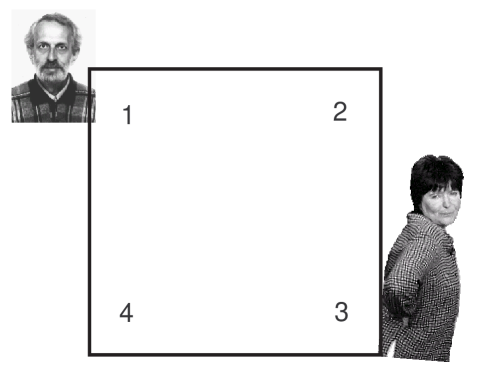
Figure 2: Alice does not see Bob and is very dissatisfied

In order to see clearly the difference between the two games and to discriminate ”wise Alice” from the ”foolish” one we introduce notations making the difference evident. Encode the strategies of Alice and Bob by vectors, consisting of zeros and ones:

$$\alpha=(\alpha_{1},\alpha_{2},\alpha_{3},\alpha_{4}),\qquad\beta=(\beta_{1},\beta_{2},\beta_{3},\beta_{4})$$

so that the component equal to one means the applied pure strategy. Then it is evident that

$$\sum_{j=1}^{4}{\alpha_{j}}=\sum_{j=1}^{4}{\beta_{j}}=1,\qquad\alpha_{j}\cdot\alpha_{k}=\beta_{j}\cdot\beta_{k}=\delta_{jk}$$

and the profit of Alice in one turn of any of the games considered is

$${\cal H}_{A}(\alpha,\beta)=\sum_{j,k=1}^{4}{h_{jk}\alpha_{j}\beta_{k}}$$ (2)

So, in the separate turn the ”wise” Alice is not different from the ”foolish” one. The difference occurs in the behaviour when the game is repeated many times. The source of the difference is in the different method of calculation of the average payoff.

Consider it explicitly. At first let us take the classical case of interaction. In the case of the ”foolish” Alice the initial strategies of Bob are not correlated with the strategies of his partner, so

$$E(\alpha_{j}\cdot\beta_{k})=E\alpha_{j}\cdot E\beta_{k}$$

and averaging of the payoff gives the well known classical expression

$$E{\cal H}_{A}(\alpha,\beta)=\sum_{j,k=1}^{4}{h_{jk}E\alpha_{j}\cdot E\beta_{k}}=\sum_{j,k=1}^{4}{h_{jk}x_{j}y_{k}}={\cal H}_{A}(x,y),$$

where $x_{j},y_{k}$ are frequencies of the corresponding pure strategies. For our payoff matrix one obtains the expression of the payoff function for Alice as

$${\cal H}_{A}(x,y)=ax_{1}y_{3}+bx_{2}y_{4}+cx_{3}y_{1}+dx_{4}y_{2}$$ (3)

Then one must, using the linear programming, find the saddle points for natural constrains

$$x_{1}+x_{2}+x_{3}+x_{4}=1,\quad y_{1}+y_{2}+y_{3}+y_{4}=1,\qquad x_{j},\,y_{k}\geqslant 0.$$

In our case there is only one equilibrium point and the mixed strategies of Alice and Bob are found as:

$$x=(\mu a^{-1},\;\mu b^{-1},\;\mu c^{-1},\;\mu d^{-1}),\qquad y=(\mu c^{-1},\;\mu d^{-1},\;\mu a^{-1},\;\mu b^{-1}),$$

where $\mu={(a^{-1}+b^{-1}+c^{-1}+d^{-1})}^{-1}$ is the price or the value of the game i.e. the average profit of Alice in the equilibrium situation. So the optimal frequency of Bob’s being in this or that corner of the building is inversely proportional to the sum of money which he must he give to his girl friend. The optimal strategy of Alice is more sophisticated: she must not be very greedy and more frequently come to the places where her friend will not pay too much to her.

Instead let us write the expression of the payoff function of the ”foolish” Alice in a somehow different form, useful for our subsequent considerations. Consider random events $\alpha_{13},\,\alpha_{24}\subset{\cal S}_{A},\;\;\beta_{13},\,\beta_{24}\subset{\cal S}_{B},$ where ${\cal S}_{A},\,{\cal S}_{B}=\{1,2,3,4\}$ – the sets of pure strategies of Alice and Bob. Each of the considered events corresponds to the choice of the pair of opposite corners of the house. It is easy to see that events $\alpha_{jk}\cap\beta_{lm}$ form the ${\cal S}_{A}\times{\cal S}_{B}$ division of the space of the game situations and thus form a complete set of events. Taking this into account one can write the payoff function for Alice as the mixture of conditional expectation values.

$${\cal H}_{A}(x,y)=\sum_{jk,lm}{E_{\alpha_{jk}\cap\beta_{lm}}{\cal H}_{A}\cdot P(\alpha_{jk}\cap\beta_{lm})}$$

In the case of our payoff matrix this expression has the form

$$(ap_{13}^{1}q_{13}^{3}+cp_{13}^{3}q_{13}^{1})\cdot P(\alpha_{13}\cap\beta_{13})+(bp_{24}^{2}q_{24}^{4}+dp_{24}^{4}q_{24}^{2})\cdot P(\alpha_{24}\cap\beta_{24}),$$ (4)

where $p_{jk}^{l},\,q_{jk}^{l}$ – conditional probabilities of the choice of the corner $l$ from the given pair of opposite corners $\{j,k\}$. From this it follows that the conditional average payoff for Alice will be

$$E_{\alpha_{13}\cap\beta_{13}}{\cal H}_{A}=ap_{13}^{1}q_{13}^{3}+cp_{13}^{3}q_{13}^{1}$$ (5)

if both players choose the diagonal $\{1,3\}$ and

$$E_{\alpha_{24}\cap\beta_{24}}{\cal H}_{A}=bp_{24}^{2}q_{24}^{4}+dp_{24}^{4}q_{24}^{2}$$ (6)

if they prefer the diagonal $\{2,4\}$. If the players choose different diagonals of the house the conditional payoff is equal to zero because in this case it is always possible for Alice to see Bob and he must not pay for presents. Easy calculations show that

$$P(\alpha_{jk}\cap\beta_{jk})=(x_{j}+x_{k})(y_{j}+y_{k}),\quad p_{jk}^{l}=\frac{x_{l}}{x_{j}+x_{k}},\quad q_{jk}^{l}=\frac{y_{l}}{y_{j}+y_{k}}$$

These formulas will be of use for us when we discuss the behaviour of Bob moving the ball in the game ”Wise Alice”.

4 .  Different logics – different behaviour

Let us discuss now the behaviour of players in the game ”Wise Alice”. First notice that this game gives the simplest model of measurement (defining the place of the object). Alice wants to know where is Bob located but she makes Bob active by her questions, ”preparing” him in a definite ”state”. She gets exact information, not in all cases, but only when the negative answer is obtained. Alice makes proposals but the logic of her propositions must be somehow different from the classical scheme. More explicitly, let $\alpha_{k}$ is the proposition of Alice that Bob’s ball is located on vertex number $k$. One can consider this value as the predicate: the function defined on the set $S_{B}$ of initial strategies of Bob taking logical values 0 or 1. For our box with a ball Fig. 1 it is easy to see that the values of propositions of Alice are distributed as follows:

$$\alpha_{1}(1)=\alpha_{1}(2)=\alpha_{1}(4)=1,\quad\alpha_{1}(3)=0,$$

$$\alpha_{2}(2)=\alpha_{2}(1)=\alpha_{2}(3)=1,\quad\alpha_{2}(4)=0,$$ (7)

$$\alpha_{3}(3)=\alpha_{3}(2)=\alpha_{3}(4)=1,\quad\alpha_{3}(1)=0,$$

$$\alpha_{4}(4)=\alpha_{4}(1)=\alpha_{4}(3)=1,\quad\alpha_{4}(2)=0.$$

Defining disjunction as usual as

$$\alpha_{j}\vee\alpha_{k}=\max(\alpha_{j},\alpha_{k})$$

one obtains a ”slight” breaking of the classical logic: the disjunction of any pair of different propositions occurs to be identically true:

$$\alpha_{j}\vee\alpha_{k}=1,\qquad j\neq k$$

Remember that for the classical ”foolish” Alice one has

$$\alpha_{1}\vee\alpha_{2}\vee\alpha_{3}\vee\alpha_{4}=1$$

Differences with classical logic occur also for negation. Instead of the classical relations $\neg\alpha_{j}=1-\alpha_{j}$ one has the equalities:

$$\neg\alpha_{1}=\alpha_{3},\quad\neg\alpha_{3}=\alpha_{1},\quad\neg\alpha_{2}=\alpha_{4},\quad\neg\alpha_{4}=\alpha_{2}$$

Really, every time when Alice learns that the Bob’s ball is not located at the questioned vertex of the square she understands that it is located at the opposite vertice. Notice that the law of double negation $\neg(\neg\alpha_{j})=\alpha_{j}$ as well as the law of the excluded third $\alpha_{j}\vee(\neg\alpha_{j})=1$ are valid. One must define the conjunction. It can be introduced by the standard formula

$$\alpha_{j}\wedge\alpha_{k}=\neg((\neg\alpha_{j})\vee(\neg\alpha_{k}))$$

It is easy to see that this is the only way of defining the conjunction if De Morgan’s laws of duality are valid:

$$\neg(\alpha_{j}\wedge\alpha_{k})=(\neg\alpha_{j})\vee(\neg\alpha_{k}),\qquad\neg(\alpha_{j}\vee\alpha_{k})=(\neg\alpha_{j})\wedge(\neg\alpha_{k})$$

Defining thus all logical operations let us check other differences with classical Boolean logic. First notice that in spite of the fact that any pair of different propositions of Alice is in complementarity:

$$\alpha_{j}\vee\alpha_{k}=1,$$

$$\alpha_{j}\wedge\alpha_{k}=0,$$

not all of them are orthocomplemented– mutually opposite. Only pairs of propositions with the same ”parity” $\{\alpha_{1};\alpha_{3}\}$ $\{\alpha_{2};\alpha_{4}\}$ are orthocomplemented. Second, one has a breaking of the distributivity law. So, for any triple of different $j,k,l$ one has the inequality

$$(\alpha_{j}\vee\alpha_{k})\wedge\alpha_{l}\neq(\alpha_{j}\wedge\alpha_{l})\vee(\alpha_{k}\wedge\alpha_{l})$$

Really, the left side of the inequality is equal to $\alpha_{l}$,while the right side is zero. So the logic of Alice occurs to be a non-distributive orthocomplemented lattice [14, 15]. Same concerns the logic of Bob. His state reduced by the question of Alice is described by the analogous system of predicates $\beta_{1},\beta_{2},\beta_{3},\beta_{4}$ defined on the set of strategies of Alice and taking the value 1 for those questions on which he can answer affirmatively. In Fig. 3 a Hasse diagram is shown describing the nondistributive logic of our players. In spite of the logical differences of introduced predicates $\alpha_{1},\alpha_{2},\alpha_{3},\alpha_{4}$ and $\beta_{1},\beta_{2},\beta_{3},\beta_{4}$ from the classical ones one can think that the payoff of Alice in the separate turn of the game still is given by the same expression as before

$${\cal H}_{A}(\alpha,\beta)=\sum_{j,k=1}^{4}{h_{jk}\alpha_{j}\beta_{k}}$$

The main difficulties arise when one goes to the repeated game and when one tries to calculate the average payoff. If one tries to give to the average value of predicates the probabilistic interpretation:

$$E\alpha_{j}=x_{j},\qquad E\beta_{k}=y_{k},$$

one immediately comes to the contradiction: the sum of probabilities of pair-wise disjoint (due to our definition of the conjunction) outcomes is larger than unity

$$x_{1}+x_{2}+x_{3}+x_{4}=3,\qquad y_{1}+y_{2}+y_{3}+y_{4}=3.$$

This follows from the additivity of the average and (8), leading to the following identities

$$\alpha_{1}+\alpha_{2}+\alpha_{3}+\alpha_{4}=3,\qquad\beta_{1}+\beta_{2}+\beta_{3}+\beta_{4}=3$$

Hope for the validity of additivity for pairs of mutually neglecting events also occurs to be in vain. Due to the property that the left-handed side of easily checked inequalities

$$\alpha_{1}+\neg(\alpha_{1})\geqslant I,\quad\alpha_{2}+\neg(\alpha_{2})\geqslant I,\quad\alpha_{3}+\neg(\alpha_{3})\geqslant I,\quad\alpha_{4}+\neg(\alpha_{4})\geqslant I$$ (8)

sometimes takes the value equal to 2, the main property of probability is broken even for orthocomplemented elements. The probability properties are also broken for the disjunction (see Hasse diagram Fig. 3).

Figure 3: Lattice of Alice’s questions and Bob’s answers

If one considers all outcomes equally possible, then the probability of the always true event, i.e. disjunction of any of two events occurs to be one half! So a classical probabilistic description of the behaviour of the players in the repeated game is impossible in principle. The solution for the situation arising is given by the ideas of quantum mechanics.

5 .  To averages through quantization

Following A.A.Grib and R.R.Zapatrin[1] we pay attention to the fact that the ortholattice of the logic of interaction of partners of the ”Wise Alice” is isomorphic to the ortholattice of invariant subspaces of the Hilbert space of the quantum system with spin $\frac{1}{2}$ and observables of the type of $S_{x}$ $S_{\theta}$.

Figure 4: Lattice of invariant subspaces of observables $S_{x}$ and $S_{\theta}$

In Fig. 4 two pairs of mutually orthogonal direct lines $\{a1;a3\}$, $\{a2;a4\}$ are shown. One of these pairs makes diagonal the operator $S_{x}$, the other $S_{\theta}$. If one takes as representations of logical conjunction and disjunction their intersection and linear envelope and if negation corresponds to the orthogonal complement one obtains the ortholattice isomorphic to the logic of our players. One example of such an isomorphism is the mapping $\alpha_{j}\mapsto aj,\;j=1,2,3,4$. We saw that in one ”experiment” neither Alice nor Bob have a stable strategy. However if the game is repeated many times one can ask about optimal frequencies of the corresponding pure strategies. Due to the non-distributivity of the logic ,as we saw previously, it is impossible to define on the sets $S_{A}$ and $S_{B}$ of pure strategies a probabilistic measure. The main problem is calculation of an adequate procedure of averaging.

Following well known constructions of quantum mechanics we take instead of the sets of pure strategies of Alice and Bob $S_{A},S_{B}$ the pair of two-dimensional Hilbert spaces $H_{A},H_{B}$. So pure strategies are represented by one-dimensional subspaces or normalised vectors of Hilbert space (wave functions). Use of Hilbert space permits us without any difficulties to realise the non-distributive logic of our players. For this one must represent predicates $\alpha_{1},\alpha_{2},\alpha_{3},\alpha_{4},$ $\beta_{1},\beta_{2},\beta_{3},\beta_{4}$ describing questions of Alice and locations of Bob’s ball by the corresponding self-conjugate operators. It is important to notice that the ortholattice can be realised in an infinite set of ways. Describe all these ways up to the unitary equivalence. We do this for the predicates of Alice. The same can be done for Bob. In $H_{A}$ take an arbitrary one-dimensional subspace and put its orth-projector into correspondence to the predicate $\alpha_{1}$: the projector denote as $\widehat{\alpha}_{1}$. To the predicate $\alpha_{3}$ put into correspondence the orthogonal complementary projector $\widehat{\alpha}_{3}$. Then the following evident and for us desirable relations are valid:

$$\widehat{\alpha}_{1}\cdot\widehat{\alpha}_{3}=\widehat{\alpha}_{3}\cdot\widehat{\alpha}_{1}=O,\qquad\widehat{\alpha}_{1}+\widehat{\alpha}_{3}=I$$ (9)

It is clear that the choice of these operators is unique up to unitary equivalence. Take an arbitrary one-dimensional subspace different from the eigenspaces of the projector $\widehat{\alpha}_{1}$ and put it into correspondence to the predicate of some orth-projector $\widehat{\alpha}_{2}$. To the variable $\alpha_{4}$ put the projector $1-\widehat{\alpha}_{2}$ . In the result one obtains one more resolution of Hilbert space $~{}H_{A}$

$$\widehat{\alpha}_{2}\cdot\widehat{\alpha}_{4}=\widehat{\alpha}_{4}\cdot\widehat{\alpha}_{2}=O,\qquad\widehat{\alpha}_{2}+\widehat{\alpha}_{4}=I$$ (10)

Projectors from different resolutions do not commute one with another. However there is a simple connection between them: the second of direct resolutions is obtained from the first by rotation through an angle different from multiples of $90^{o}$. In other words there exists a unitary operator $~{}u~{}$ such that

$$\widehat{\alpha}_{2}=u^{-1}\widehat{\alpha}_{1}u,\qquad\mbox{ }\qquad\widehat{\alpha}_{4}=u^{-1}\widehat{\alpha}_{3}u$$ (11)

It is clear that this unitary operator defines the class of unitary equivalent realisations of our non-distributive ortholattice, negation is represented by going to the complementary projector. Notice that differently from the predicative description due to rules (7) leading to unpleasant inequalities (8) the operator representation of the non-distributive lattice due to (9,10) is ”friendly” to orthocomplementarity:

$$\widehat{\alpha}_{1}+(\widehat{\alpha}_{1})^{\bot}=I,\quad\widehat{\alpha}_{2}+(\widehat{\alpha}_{2})^{\bot}=I,\quad\widehat{\alpha}_{3}+(\widehat{\alpha}_{3})^{\bot}=I,\quad\widehat{\alpha}_{4}+(\widehat{\alpha}_{4})^{\bot}=I$$

Doing the same for the Bob’s lattice one comes to the observables $\widehat{\beta_{1}},\widehat{\beta_{2}},\widehat{\beta_{3}},\widehat{\beta_{4}}$ and analogous to $~{}u~{}$ a unitary operator $~{}v~{}$ giving the connections between ”even” and ”odd” variables. The next step of our scheme is the space of game situations. The quantum analog of the classical space of game situations becomes the tensor product ${\sf H}_{A}\otimes{\sf H}_{B}$. This space is necessary for introducing the main observable: the payoff for Alice. To write this observable following quantum mechanics take the classical expression (3) of the payoff function of Alice

$${\cal H}_{A}(\alpha,\beta)=\sum_{j,k=1}^{4}{h_{jk}\alpha_{j}\beta_{k}}$$

and write there the corresponding projectors. In the result one obtains the self-conjugate operator in ${\sf H}_{A}\otimes{\sf H}_{B}$, the observable of the payoff for Alice:

$$\widehat{{\cal H}}_{A}=\sum_{j,k=1}^{4}h_{jk}\widehat{\alpha}_{j}\otimes\widehat{\beta}_{k}$$

Let Alice and Bob repeat their game with a ball many times and let us describe theirbehaviour by normalised vectors $\varphi\in{\sf H}_{A},\;\mbox{ }\;\psi\in{\sf H}_{B}$. The element $s=\varphi\otimes\psi$ expressing their interaction during the game is a normalised vector in ${\sf H}_{A}\otimes{\sf H}_{B}$. Taking it as the characteristic of the state of the game calculate the average in this state $E_{\varphi\otimes\psi}\widehat{{\cal H}}_{A}$ according to the standard rules of quantum mechanics

$$\langle\widehat{{\cal H}}_{A}s,\,s\rangle=\sum_{j,k=1}^{4}{h_{jk}\langle(\widehat{\alpha}_{j}\otimes\widehat{\beta}_{k})\;\varphi\otimes\psi,\;\varphi\otimes\psi\rangle}$$

so that after easy transformations one gets for the average payoff for the given types of behaviour of the players:

$$E_{\varphi\otimes\psi}\widehat{{\cal H}}_{A}=\sum_{j,k=1}^{4}{h_{jk}\langle\widehat{\alpha}_{j}\varphi,\,\varphi\rangle\cdot\langle\widehat{\beta}_{k}\psi,\,\psi\rangle}$$

Putting into this formula the elements of our payoff matrix and using the notations $~{}p_{j}=\langle\widehat{\alpha}_{j}\varphi,\,\varphi\rangle~{}$, $~{}q_{k}=\langle\widehat{\beta}_{k}\psi,\,\psi\rangle~{}$ one obtains

$$E_{\varphi\otimes\psi}\widehat{{\cal H}}_{A}=ap_{1}q_{3}+cp_{3}q_{1}+bp_{2}q_{4}+dp_{4}q_{2}$$ (12)

It is useful to compare this expression with the classical average obtained earlier for the ”foolish” Alice:

$${\cal H}_{A}(x,y)=ax_{1}y_{3}+cx_{3}y_{1}+bx_{2}y_{4}+dx_{4}y_{2}$$

There is some resemblance but there is also a serious difference. One could ask, why it is impossible to recalculate the quantum average differently by normalising the frequencies to one not only for each diagonal separately but for two diagonals as it is made in the classical case? But the fact is that like in case of measuring non-commuting operators of spin projections Alice knows about her interaction with Bob when she asks him and receives the answer. This interaction is different when questions on different diagonals are asked because different positions of the ball are immovable for these cases. So relative to different interactions (different context) different events are defined leading to different probabilistic spaces as it is true for measuring spin projections. One can use the metaphor that if in one case Alice is throwing the coin and is interested if ”up” or ”down” will arise, in the other case the interaction with Alice will change the coin in such a way as if a new coin is thrown, on one side of which a big ”up” and the small ”down” of the previous coin are drawn. On the other side of the new coin the opposite situation occurs. So the new coin is made asymmetric following the structure of the payoff matrix. In homogeneity of events in the quantum case makes impossible the renormalisation of frequencies and leads to new results for averages.

6 .  Probability amplitudes instead of probabilities

The main difference in the given formulas is in the sense of variables. If $x_{j},x_{k}$ are probabilities, the $~{}p_{j},p_{k}~{}$ cannot be because they contradict the main laws of the probability theory. Really, taking into account that the projectors $\widehat{\alpha}_{j}$ and $\widehat{\beta}_{k}$ with indices of the same parity commute and form a resolution of unity, one obtains after standard calculations the following identities.

$$p_{1}+p_{3}=\langle\widehat{\alpha}_{1}\varphi,\,\varphi\rangle+\langle\widehat{\alpha}_{3}\varphi,\,\varphi\rangle=\langle(\widehat{\alpha}_{1}+\widehat{\alpha}_{3})\,\varphi,\varphi\rangle=1,$$ (13)

$$p_{2}+p_{4}=1,\quad q_{1}+q_{3}=1,\quad q_{2}+q_{4}=1$$ (14)

So, differently from classical probability theory, for each family of pairwise disjoint events $\{\widehat{\alpha}_{j}\},\,\{\widehat{\beta}_{k}\}$ one obtains the relations

$$p_{1}+p_{2}+p_{3}+p_{4}=2,\qquad q_{1}+q_{2}+q_{3}+q_{4}=2$$

The sense of the values $~{}p_{j},p_{k}$ is obtained by using the standard quantum rule. Let for example the behaviour of Alice be described by the normalized vector $\varphi\in{\sf H}_{A}$, and let $\xi_{1}^{+},\xi_{1}^{-}\in{\sf H}_{A}$ be normalised eigenvectors of the projector with eigenvalues 1 (”yes”) and 0 (”no”). Projecting the state vector of Alice onto the basis $\{\xi_{1}^{+},\xi_{1}^{-}\}$

$$\varphi=c_{+}\xi_{1}^{+}+c_{-}\xi_{1}^{-}$$

one obtains that she can find Bob’s ball on the first vertex of the square with the probability

$$p_{1}=\langle\widehat{\alpha}_{1}(c_{+}\xi_{1}^{+}+c_{-}\xi_{1}^{-}),\;c_{+}\xi_{1}^{+}+c_{-}\xi_{1}^{-}\rangle=\langle c_{+}a_{1}^{+},\;c_{+}\xi_{1}^{+}+c_{-}\xi_{1}^{-}\rangle=|c_{+}|^{2}$$

and on the opposite vertex with the probability $p_{3}=|c_{-}|^{2}$. So the numbers $~{}p_{j},p_{k}$ must be interpreted due to quantum mechanics as the squares of moduli of probability amplitudes. The identities obtained by us earlier for the classical game make it possible to compare each of the four pairs of numbers $\{p_{1},p_{3}\}$, $\{p_{2},p_{4}\}$, $\{q_{1},q_{3}\}$, $\{q_{2},q_{4}\}$ separately with the corresponding conditional probabilities. Compare formula(12)for the quantum average

$$E_{\varphi\otimes\psi}\widehat{{\cal H}}_{A}=(ap_{1}q_{3}+cp_{3}q_{1})+(bp_{2}q_{4}+dp_{4}q_{2})$$

with formula (4) used for calculation of the classical average by the use of conditional probabilities and conditional expectation values:

$$E{\cal H}_{A}=(ap_{13}^{1}q_{13}^{3}+cp_{13}^{3}q_{13}^{1})\cdot P_{13}+(bp_{24}^{2}q_{24}^{4}+dp_{24}^{4}q_{24}^{2})\cdot P_{24}$$ (15)

In the case when the corresponding pairs of the squares of moduli of amplitudes are equal to classical conditional probabilities

$$p_{1}=p_{13}^{1},\quad p_{3}=p_{13}^{3},\quad p_{2}=p_{24}^{2},\quad p_{4}=p_{24}^{4}$$

$$q_{1}=q_{13}^{1},\quad q_{3}=q_{13}^{3},\quad q_{2}=q_{24}^{2},\quad q_{4}=q_{24}^{4}$$

one obtains an interesting result: the ”wise” Alice gets a larger payoff than that which is obtained by her ”foolish” copy:

$$E_{\varphi\otimes\psi}\widehat{{\cal H}}_{A}\geqslant E{\cal H}_{A}$$

Notice, however, that to have this one must have the situation where the squares of moduli of the probability amplitudes in ”quantum” Nash equilibrium are equal to the conditional probabilities obtained by applying the apparatus of the classical game theory. However there is no foundation for such an equality. In fact, if the equilibrium point of the classical game is searched on the set of nonnegative numbers with constrains

$$x_{1}+x_{2}+x_{3}+x_{4}=1,\qquad y_{1}+y_{2}+y_{3}+y_{4}=1$$

then in the quantum game case for the squares of moduli of the probability amplitudes besides the explicit linear relations

$$p_{1}+p_{3}=1,\qquad p_{2}+p_{4}=1,\qquad q_{1}+q_{3}=1,\qquad q_{2}+q_{4}=1$$

there are implicit relations due to unitary dependence (12) of projection operators with even and odd indices. The difference between the two pictures is due to the fact that in the quantum situation the formula of full probability (15) is broken: the average payoff to Alice is equal to the sum of conditional probabilities and not to their mixture: $~{}P_{13}=P_{24}=1$. This again demonstrates that it is impossible to find a quantum equilibrium point by use of only formula (13) of the average payoff as a function of eight variables $\{p_{j},q_{k}\}$ with the relations written before between them. The equilibrium is defined not by the combination of the squares of moduli of the amplitudes of Alice and Bob but by the combination of wave functions $\varphi\in{\sf H}_{A}$ and $\psi\in{\sf H}_{B}$.

7 .  Behaviour of the player as realisation of logic

Besides the amplitudes, characterising the behaviour of players, our model has two additional structural characteristics: unitary rotations $~{}u~{}$ and $~{}v~{}$, giving an operator representation of the ortholattices of Alice and Bob up to unitary equivalence. Each of these operators can be characterised by the angle between eigensubspaces of even and odd order. Denote by $\theta_{A}$ the angle between direct lines corresponding to the largest eigenvectors of operators $\widehat{\alpha}_{1}$ , $\widehat{\alpha}_{2}$ of Alice and $\theta_{B}$ the analogous angle characterising the realisation of the logic of Bob. Differently from the amplitudes characterising the behaviour of the players, being the variables of the model, the angles are its parameters.These parameters characterise the type of player, making it possible to consider logic as some factor forming the behaviour. Some sense of these values can be the following: the angles characterise the connections between choices of the diagonals of the square or some preferences for this or that adjacent vertex. The angles $\theta_{A},~{}\theta_{B}$ define commutation relations for corresponding operators. Consider for example the operators $\widehat{\alpha}_{1}$, $\widehat{\alpha}_{2}$. Taking as an orthonormal basis in the space $~{}H_{A}~{}$of Alice the eigenbasis of the operator $\widehat{\alpha}_{1}$ let us write the matrices of this pair of operators

$$\widehat{\alpha}_{1}=\rm\left(\begin{array}[]{rr}1&0\\ 0&0\\ \end{array}\right),\hskip 30.0pt\widehat{\alpha}_{2}=\rm\left(\begin{array}[]{lr}\cos^{2}{\theta}_{A}&\sin{\theta}_{A}\cos{\theta}_{A}\\ \sin{\theta}_{A}\cos{\theta}_{A}&sin^{2}{\theta}_{A}\\ \end{array}\right)$$

where $\theta_{A}$ is the angle on which eigenbasis of the operator $\widehat{\alpha}_{2}$ is rotated relative to the eigenbasis of the operator $\widehat{\alpha}_{1}$. Calculating the commutator of these matrices one obtains:

$$[\widehat{\alpha}_{1},\,\widehat{\alpha}_{2}]=\frac{i}{2}\cdot\sin 2\theta_{A}\rm\left(\begin{array}[]{rr}0&-\,i\\ i&0\\ \end{array}\right)$$

Analogous commutation relations are obtained for Bob’s operators. Non-commutativity of the operators of the logic representation expresses evident, without any mathematics, the dependence of the results of the game on the order of acts. So Bob’s state is different depending on the order: ”1”, then ”2” or ”2”, then ”1”, in which he received Alice’s questions . So in the quantum model one takes into account not only the interests of the players represented in the payoff matrix but in some sense their personal features on which depends the level of realisation of interests.

8 .  In search of the quantum equilibrium.

The definition of the Nash equilibrium for the quantum case is not much different from the classical case (1) and can be written as

$$E\widehat{{\cal H}}_{A}(\varphi^{0},\psi^{0})\geqslant E\widehat{{\cal H}}_{A}(\varphi,\psi^{0}),\qquad E\widehat{{\cal H}}_{B}(\varphi^{0},\psi^{0})\geqslant E\widehat{{\cal H}}_{B}(\varphi^{0},\psi)$$

It is convenient to find the equilibrium points in the coordinate form. To do this let us fix in the space of strategies of Alice $~{}H_{A}~{}$ eigenbases $\{\xi_{1}^{+},\xi_{1}^{-}\}$ $\{\xi_{2}^{+},\xi_{2}^{-}\}$ corresponding to two projectors $\widehat{\alpha}_{1},\widehat{\alpha}_{2}$ and let us do the same for Bob, taking bases $\{\eta_{1}^{+},\eta_{1}^{-}\}$ $\{\eta_{2}^{+},\eta_{2}^{-}\}$. The angles between the largest eigenvectors denote as $\theta_{A}$ and $\theta_{B}$. Then one can write in the quantum payoff function

$$E\widehat{{\cal H}}_{A}({\varphi,\psi})=ap_{1}q_{3}+cp_{3}q_{1}+bp_{2}q_{4}+dp_{4}q_{2}$$

the squares of moduli of the amplitudes $~{}p_{j},p_{k}~{}$ as

$$p_{1}=\cos^{2}\alpha,\quad p_{3}=\sin^{2}\alpha,\quad p_{2}=\cos^{2}(\alpha-\theta_{A}),\quad p_{4}=\sin^{2}(\alpha-\theta_{A}),$$

$$q_{1}=\cos^{2}\beta,\quad q_{3}=\sin^{2}\beta,\quad q_{2}=\cos^{2}(\beta-\theta_{B}),\quad q_{4}=\sin^{2}(\beta-\theta_{B}),$$

where $\alpha,\beta$ are the angles of vectors $\varphi,\psi$ to the corresponding axises. For values of angles one can take the interval $[0^{0};180^{0}]$. In the result the problem of search of the equilibrium points of the quantum game became the problem of finding a minimax of the function of two angle variables

$$F(\alpha,\beta)=a\cos^{2}\alpha\sin^{2}\beta+c\sin^{2}\alpha\cos^{2}\beta+$$

$$+b\cos^{2}(\alpha-\theta_{A})\sin^{2}(\beta-\theta_{B})+d\sin^{2}(\alpha-\theta_{A})\cos^{2}(\beta-\theta_{B})$$

on the square $[0^{0};180^{0}]\times[0^{0};180^{0}]$. In other words our quantum game occurred to be an infinite antagonistic game of two persons on the square. Solving such games in pure strategies, i.e. search for saddle points of the function $F(\alpha,\beta)$ is a difficult problem. It is known [16] that for the existence of the saddle points properties of continuity and smoothness of the payoff function are not enough. Present theorems of existence use properties of convexity of this function. However in our case we don’t have these properties. One can find examples of some values of the elements $a,b,c,d$ of the payoff matrix (9) when the function $F(\alpha,\beta)$ doesn’t have saddle points. Not much better is the situation with methods of search of the saddle points. Differently from the geometrical saddle points the conditions of the Nash equilibrium are not just putting to zero values of the corresponding partial derivatives. So in the situation of absence of simple analytical solutions one must look for numerical methods. To do calculations we use an algorithm based on the construction of ”curves of reaction” or ”curves of the best answers” of the participants of the game.

The definition of curves of reaction is based on the following consideration. If Alice knew what decision Bob will take she could make an optimal choice. But the essence of the game situation is that she doesn’t know it. She must take into account his different strategies and on each possible act of the partner she must find the optimal way to act. Her considerations look like considerations of the player, expressed by the formula: ”if he does this, then I shall do that”. Bob thinks the same way. So one must consider two functions $\alpha={\cal R}_{A}(\beta)$ and $\beta={\cal R}_{B}(\alpha)$ the plots of which are called the curves of reactions of Alice and Bob. Due to the definition of these functions

$$\max_{\alpha}F(\alpha,\,\beta)=F({\cal R}_{A}(\beta),\,\beta),\qquad\min_{\beta}F(\alpha,\,\beta)=F(\alpha,\,{\cal R}_{B}(\alpha))$$

It is easy to see that intersections of curves of reaction give points of Nash equilibrium. Numerical experiments show that dependent on the values of the parameters $a,b,c,d$ of the payoff function and the angles characterising the type of player one has qualitatively different pictures. Intersections can be absent, there can be one intersection and lastly there can be the case with two equilibrium points with different values of the payoff of the game, which is absent in the case of the classical matrix game.

9 .  Examples

1. Two equilibrium points arise in the case of the payoff matrix:

$A\backslash B$	1	2	3	4
1	0	0	3	0
2	0	0	0	3
3	5	0	0	0
4	0	1	0	0

and an operator representation of the ortholattice corresponding to angles $\theta_{A}=10^{0}$, $\theta_{B}=70^{0}$. One of the equilibrium points is inside the square, the other one is on it’s boundary (see Fig. 5).

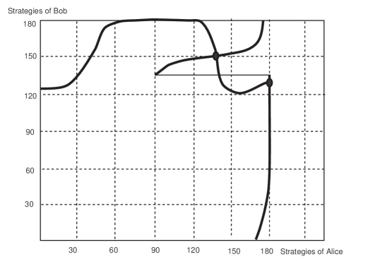
Figure 5: Two points of Nash equilibrium

The curves of reaction in this case happen to be discontinuous. For convenience the discontinuities are shown by thin lines. The discontinuous character of the curve of reaction of Alice made it impossible for one more equilibrium point to occur. One of the equilibrium takes place for $\alpha=145,5^{0}$, $\beta=149,5^{0}$ and gives the following values for the squares of moduli of amplitudes:

for Alice $p_{1}=0,679;p_{2}=0,509;p_{3}=0,321;p_{4}=0,491;$

for Bob $q_{1}=0,258;q_{2}=0,967;q_{3}=0,742;q_{4}=0,033.$

The price of the quantum game, i.e. the equilibrium value of the profit for Alice in this case is equal to $E\widehat{\cal H}_{A}=2.452$. The second equilibrium point corresponds to angles $\alpha=180^{0}$, $\beta=123,5^{0}$ and the squares of the amplitude moduli

for Alice $p_{1}=1.000;p_{2}=0,967;p_{3}=0.000;p_{4}=0.033;$

for Bob $q_{1}=0,695;q_{2}=0.646;q_{3}=0.305;q_{4}=0.354.$

The price of the game in the second equilibrium point is equal to $E\widehat{\cal H}_{A}=1.926$. For the classical game with the same payoff matrix (see section 4) the price of the game happens to be smaller and is equal to ${15\over 28}$ = $0.536.$ Differently from the quantum game the classical game has onlyone equilibrium point which is obtained for the following frequencies

for Alice $x_{1}={5\over 28}$; $x_{2}={5\over 28}$; $x_{3}={3\over 28}$; $x_{4}={15\over 28};$

for Bob $y_{1}={3\over 28}$; $y_{2}={15\over 28}$; $y_{3}={5\over 28}$; $y_{4}={5\over 28}$.

To compare the quantum game with the classical one the conditional probabilities for the choice of vertices of the square after the choice of the diagonal are found to be:

for Alice: $p^{1}_{13}={5\over 8}$; $p^{3}_{13}={3\over 8}$; $p^{2}_{24}={1\over 4}$; $p^{4}_{24}={3\over 4}$;

for Bob : $q^{1}_{13}={3\over 8}$; $q^{3}_{13}={5\over 8}$; $q^{2}_{24}={3\over 4}$; $q^{4}_{24}={1\over 4}$;

and the conditional average payoffs (5,6) for each diagonal are:

$$~{}E_{13}{\cal H}_{A}=1.875;\qquad E_{24}{\cal H}_{A}=0.75.$$

The price of the classical game is obtained by multiplication of these expressions on the probabilities of the corresponding conditions given in section(4). Terms of the quantum payoff, associated with these conditional averages $E_{\varphi\otimes\psi}\widehat{{\cal H}}_{A}$ in case of the first equilibrium point are

$~{}ap_{1}q_{3}+cp_{3}q_{1}=1.927~{};$  $~{}bp_{2}q_{4}+dp_{4}q_{2}=0.525~{}$

For the second equilibrium point one has:

$ap_{1}q_{3}+cp_{3}q_{1}=0.915$ ; $bp_{2}q_{4}+dp_{4}q_{2}=1.048$.

2. A unique equilibrium is observed for example in the case when all nonzero payoffs are equal and are equal to one and for equal angles $\theta_{A}=45^{0}$, $\theta_{B}=45^{0}$. The equilibrium point is located in the upper right vertex of the square (see Fig. 6):

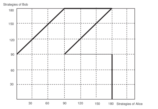
Figure 6: The unique Nash equilibrium

The curve of Bob’s reaction is shown on the Fig. 6 as continuous while the analogous curve of Alice is discontinuous when Bob is using the strategy corresponding to the angle $\beta=90^{0}$. To make it more explicit the discontinuity is shown by drawing the thin line. In reality both lines are discontinuous. This becomes evident if one prolongs both functions on the whole real axis taking into account the periodicity: the plots of one of them is obtained by the shift of the other one on the halfperiod-$90^{0}$. The squares of the amplitude moduli in this case have the following values

for Alice: $~{}p_{1}=1~{}$; $~{}p_{2}=0.5~{}$; $~{}p_{3}=0~{}$; $~{}p_{4}=0.5~{}$;

for Bob: $~{}q_{1}=1~{}$; $~{}q_{2}=0.5~{}$; $~{}q_{3}=0~{}$; $~{}q_{4}=0.5~{}$.

The payoff of the ”wise” Alice in this case is $~{}E\widehat{\cal H}_{A}=0.5~{}$ while her classical copy gets only $0.125$. Differently from the quantum case for the classical players with such a payoff function all vertices of the square are equally probable.

The unique equilibrium located inside the square takes place for the initial payoff matrix $a~{}=~{}3,\;b~{}=~{}3,\;c~{}=~{}5,\;d~{}=~{}1$ and angles $\theta_{A}=15^{0}$, $\theta_{B}=35^{0}$ (see Fig. 7).

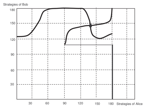
Figure 7: The other example of the unique Nash equilibrium

3. Absence of equilibrium is perhaps one of the most interesting phenomena, because as it is known for classical matrix games, equilibrium in mixed strategies always exist. One can obtain absence of equilibrium by taking the same payoff matrix for which one as well as two points of equilibrium were found. For this it is sufficient to take the operator representation of the ortholattice with typical angles: $\theta_{A}=30^{0}$, $\theta_{B}=20^{0}$ (see Fig. 8).

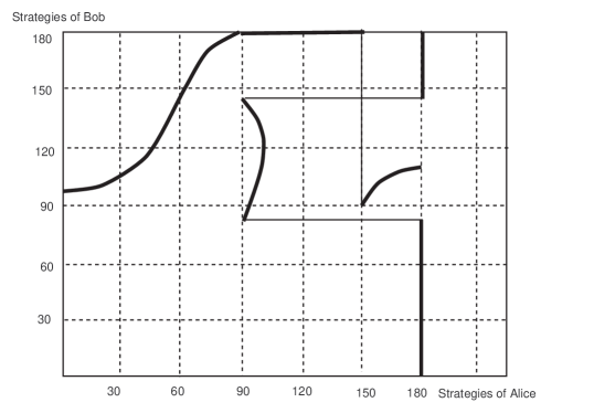
Figure 8: Absence of Nash equilibrium

Absence of equilibrium in this case as it is seen from the Fig. 8 is due to the discontinuity of the functions of reaction which is impossible in the classical case. We met this phenomenon in the first example when two equilibrium points were obtained. This last example shows the importance of the realisation of a non-distributive lattice. In the language of the game theory one can understand it as follows: having the same interests the players can form their behaviour qualitatively in different ways. So the mathematician can give to the client, for example to Alice, strategic recommendations: how she can organise the style of her behaviour to make the profit larger for the same payoff conditions. For this, however, he must know the choice of the representation of Bob’s logic.

Concluding remarks

The construction and analysis of our models show that the main difference between classical and quantum points of view on observable phenomena is expressed in the way of calculation of averages. In fact, if one remembers the first work of M.Planck on the spectra of radiation of a perfect black body one will see that the correct formula was obtained on the basis of a postulate, leading to the other than classical way of calculating oscillator average energy. Instead of the uniform distribution for degrees of freedom one used an averaging based on totally different statistics. The subsequent history of quantum physics is in some sense the history of the development of the concept of the average: important characteristics of the objects of the microworld are manifested in their ”statistics”. The development of the mathematical formalism of quantum mechanics is also strongly based on the same idea. Positive functionals on non-commutative algebras with involution in GNS construction are nothing but averages. The difference between the quantum and classical concepts of average consists in the fact that there are questions in quantum mechanics that cannot have simultaneous answers, i.e. the ortholattice of answers is not a Boolean algebra, the distributivity rule is broken in it. Practically all modern theories of quantum mechanics more or less explicitly suppose that the corresponding lattice is the lattice of closed subspaces of Hilbert space. This supposition has a constructive character and leads to operator representations and it is just this scheme of calculating the averages that was realised in this work. In what sense and what is the justification of using the apparatus of quantum mechanics in game theory when one deals with properties of macroscopic objects? The woman taking in her hand the diamond and feeling its anomalous heat capacity can know nothing about the formula of Einstein-Debye and about the specific procedure of averaging, explaining the observed phenomenon. However, one who knows it will not be surprised by the attempts to explain some features of macrophenomena by the specific way of calculating the averages. The exact answer to our question implies an analysis of the logical structure of the investigated phenomena. If the logic adequately representing the experience is non-distributive then classical procedures of calculating the averages lead, as we saw, to contradictions and one must use another apparatus. If the obtained lattice happens to be the lattice of subspaces, then the answer is given by the Gleason’s theorem [17] saying that probability measures on the lattice of projectors have strictly definite form. So if one is solving the problem of averaging of the payoff function, taking into account logical conditions of the players, then going to quantization in some cases is predestined.

One can only be surprised that the structure of the classical expression of the payoff function is such as if it were specially invented to put there instead of the two-valued function the operators. This leads to the general scheme of quantization of games. In any case if one considers not antagonistic but bimatrix game when the interests of the players are not strictly antagonistic, the scheme of quantization will be the same. This problem however as well as games of many persons goes beyond the contents of this paper. The problem of non-uniqueness of orthocomplements in the lattices is also goes beyond our paper.It exists even in case of our lattice: for negations one can take correspondence between ”even” and ”odd” questions. In the general case this problem, touching the theory of representations of internal symmetries of non-classical logics can lead also to some natural application of the formalism of quantum mechanics. The important point in our scheme is taking care in the difference between the logic and its operator representation. One sees that there exists a continuum of classes of unitary equivalent representations, parameterised by the angles of the type $\theta_{A}$, $\theta_{B}$. Each of these representations can be described by the commutation relations for the corresponding non-commuting operators. In the players logic these pairs of projectors correspond to mutually complementary questions, neither of which is the negation of the other. As it was shown previously non-commutativity is connected with the dynamics of the game – the order in which questions are posited. Considering the quantum game we had the problem of existence of equilibrium. As was seen from the examples their existence or absence is connected not only with the structure of the payoff matrix but also with the representation of the lattice of properties. Absence of equilibrium is also connected with the representation of the behaviour of the players by pure states-by vectors in Hilbert spaces, when the game situation is represented by some resolved element of their tensor product. The notion of equilibrium can be enlarged as it is done in the classical game theory taking mixed enlargement on the basis of the density matrices. Here we didn’t consider entangled states. As was shown [2] in the case of entangled states one must deal with more complex non-distributive lattices. The search of equilibrium among entangled non-factorisable states can lead to success in proving the existence of equilibrium in the general case of quantum games.

References

- [1] Grib A.A., Zapatrin R.R. Int. Journ. Th. Phys. 29 (2), (1990), p.113.
- [2] Grib A.A., Zapatrin R.R. Int. Journ. Theor. Phys. 30 (7), (1991), p.949.
- [3] Grib A.A. Breaking of Bell’s inequalities and the problem of measurement in the quantum theory. Lectures for young scientists – JINR, Dubna, (1992), (in Russian)
- [4] Grib A.A., Rodrigues Jr.W.A. Nonlocality in Quantum Physics // Kluwer Academic / Plenum Publishers – N.Y., Boston, Dodrecht, London, Moscow, (1999).
- [5] Deutsch D. Quantum Theory of Probability and Decisions. – Proc. R. Soc. Lond. Acad., (1999). (quant-ph/9906015)
- [6] Finkelstein J. Quantum Probability from Decisions Theory? – SJSU-99-20, June (1999).
- [7] Polley I. Reducing the Statistical Axiom. – Phys. Dep. Oldenburg Univ. D-26111, July (1999).
- [8] Eisert J. et all Phys. Rev. Lett. 83, (1999), p.3077.
- [9] Ekert A.K. Phys. Rev. Lett. 67, (1999), p.661.
- [10] Marinatto L., Weber T. Phys. Lett. A 272, (2000), p.291.
- [11] Moulin H. Théorie des jeux pour l’économie et la politique. – Hermann, Paris, (1981).
- [12] von Neumann J., Morgenstern O. Theory of games and economic behaviour. – Princeton. Princeton Univ. Press, (1953).
- [13] Kemeny J.D., Thompson G.L. The effect of psychological attitudes on the outcomes of games // Contributions to theory of games – 3, Princeton, (1957) pp.273-298.
- [14] Birkhoff G. Lattice Theory – AMS Colloc. Publ., vol. 25, AMS, Providence, Rhode, Island, (1993).
- [15] Grätzer G. Lattice Theory – San Francisco: Freeman & Co., (1971).
- [16] Worob’ev N.N. Foundations of Game Theory. Non-cooperative games – Birkhäuser Verlag. Basel, Boston, Berlin, (1994).
- [17] Mackey G.W. The Mathematical Foundations of Quantum Mechanics – W.A.Benjamin, INC. N.Y., Amsterdam, (1963).
- [18] Sudbery A. Quantum Mechanics and particles of nature – Cambridge. Univ. Press., (1986).
- [19] Parfionov G.N., Zapatrin R.R. Linear programming method for finding orthocomplements in finite lattices – Int. Journ. of Th. Phys, 37, (1998) pp.211-213.