Stockholm
USITP 02
June 2002
Revised November 2002

A given density matrix may be represented in many ways as a mixture of pure states. We show how any density matrix may be realized as a uniform ensemble. It has been conjectured that one may realize all probability distributions that are majorized by the vector of eigenvalues of the density matrix. We show that if the states in the ensemble are assumed to be distinct then it is not true, but a marginally weaker statement may still be true.

1. Introduction

A key property of quantum mechanics is that every mixed state, that is every non-pure density matrix, can be written as an ensemble of pure states in many ways. There exists a well known characterization of this property, apparently first published by Schrödinger [1] [2]:

Theorem 1: A density matrix ${\rho}$ having the diagonal form

$${\rho}=\sum_{i=1}^{M}{\lambda}_{i}|e_{i}\rangle\langle e_{i}|$$ (1)

can be written in the form

$${\rho}=\sum_{i=1}^{N}p_{i}|{\psi}_{i}\rangle\langle{\psi}_{i}|\ ,\hskip 22.76219pt\sum_{i=1}^{N}p_{i}=1$$ (2)

if and only if there exists a unitary $N\times N$ matrix $U$ such that

$$|{\psi}_{i}\rangle=\frac{1}{\sqrt{p}_{i}}\sum_{j=1}^{M}U_{ij}\sqrt{{\lambda}_{j}}|e_{j}\rangle\ .$$ (3)

Here all states are normalized to unit length but may not be orthogonal to each other.

Observe that the matrix $U$ does not act on the Hilbert space but on vectors whose components are state vectors, and also that we may well have $N>M$. But only the first $M$ columns of $U$ appear in the equation—the remaining $N-M$ columns are just added in order to allow us to refer to the matrix $U$ as a unitary matrix. What the theorem basically tells us is that the pure states $|{\psi}_{i}\rangle$ that make up an ensemble are linearly dependent on the $M$ vectors $|e_{i}\rangle$ that make up the so called “eigenensemble”. Moreover an arbitrary state in that linear span can be included. For definiteness we assume from now on that all density matrices have rank $M$ so that we consider ensembles of $N$ pure states in an $M$ dimensional Hilbert space.

One can say a bit more. Recall that there is a notion called “majorization” that provides a natural partial preordering of probability distributions [3]. To be precise assume that (if necessary) the eigenvalue vector $\vec{\lambda}$ has been extended with zeroes until it has the same number $N$ of components as $\vec{p}$, and also that the entries in the probability vectors have been arranged in decreasing order. (In the sequel these assumptions will often be made tacitly.) By definition the distribution $\vec{p}$ is majorized by the distribution $\vec{\lambda}$, written $\vec{p}\prec\vec{\lambda}$, if and only if

$$\sum_{i=1}^{k}p_{i}\leq\sum_{i=1}^{k}{\lambda}_{i}$$ (4)

for all $k<N$. In colloquial terms, the probability distribution $\vec{p}$ is “more even” than the distribution $\vec{\lambda}$. Now it is an easy consequence of Theorem 1 that the probability vector that appears there is given by

$$p_{i}=\sum_{j=1}^{M}B_{ij}{\lambda}_{j}\ ;\hskip 22.76219ptB_{ij}=|U_{ij}|^{2}\ .$$ (5)

The matrix $B$ is bistochastic (all its matrix elements are positive and the sum of each row and each column is unity). This follows because by construction it is unistochastic, that is each matrix element is the absolute value squared of the corresponding element of a unitary matrix. All unistochastic matrices are bistochastic, but the converse is not true. One can now show:

Theorem 2: Given a probability vector $\vec{p}$ there exists a set of pure states $|{\psi}\rangle$ such that eq. (2) holds if and only if $\vec{p}\prec\vec{\lambda}$, where $\vec{\lambda}$ is the eigenvalue vector.

In one direction this was shown by Uhlmann [4]: If such a decomposition exists then $\vec{p}\prec\vec{\lambda}$ because all vectors that can be reached from a given vector with a bistochastic matrix are majorized by the given vector [3]. The converse was shown by Nielsen, who gave an algorithm for constructing the states $|{\psi}_{i}\rangle$ given the vector $\vec{p}\prec\vec{\lambda}$ [5]. We will return to his construction below.

Why are these facts of interest? For one thing the components of $\vec{p}$ can arise as the squares of the coefficients in a Schmidt decomposition of a bipartite entangled state (and the density matrix then appears as the state of a subsystem). These theorems then give insight into the different representations that entangled states can be given. In particular Nielsen uses this insight to obtain a new protocol for the conversion of one entangled state to another by means of local operations and classical communication (LOCC) [5]. As a general remark increasing ability to manipulate quantum states in the laboratory requires increasing precision in our understanding of how they can be represented mathematically.

Now we can make a more precise statement which has not been proved:

Conjecture 1: Given any probability vector $\vec{p}$ majorized by the eigenvalue vector $\vec{\lambda}$ there exists a set of distinct pure states $|\psi_{i}\rangle$ such that eq. (2) holds.

There is no guarantee that the algorithm offered by Nielsen leads to an ensemble of distinct states. In fact, as we will show, in general it does not—indeed Conjecture 1 is false.

Our purpose is to formulate a new conjecture along the same lines that has a chance of being true. We begin in section 2 with a geometrical proof of a weak form of Conjecture 1, namely that any non-pure density matrix can be obtained as a uniform ensemble of pure states. We also explain why Conjecture 1 is in fact false. In section 3 we provide a review for physicists of the theory of majorization and bistochastic matrices. In section 4 we analyze the counterexamples to Conjecture 1 and collect some evidence for Conjecture 2, which will be a slight modification of the original. We fail to prove it though. Our conclusions are summarized in section 5.

2. Uniform ensembles

We want to construct a uniform ensemble (with all the $p_{i}$ equal to $1/N$) for an arbitrary quantum state. Provided that the state is not pure such an ensemble can be constructed with very little ado. Let ${\rho}=\mbox{diag}({\lambda}_{1},{\lambda}_{2},\ ...\ ,{\lambda}_{M})$. Choose a pure state vector whose entries are the square roots of the eigenvalues of ${\rho}$. Then form the one parameter family of state vectors

$$Z^{\alpha}({\tau})=\left(\begin{array}[]{ccc}e^{in_{1}{\tau}}&0&0\\ 0&e^{in_{2}{\tau}}&0\\ 0&0&e^{in_{3}{\tau}}\end{array}\right)\left(\begin{array}[]{c}\sqrt{{\lambda}_{1}}\\ \sqrt{{\lambda}_{2}}\\ \sqrt{{\lambda}_{3}}\end{array}\right)\ .$$ (6)

Here we choose $M=3$ for illustrative purposes and the notation anticipates the fact that we will choose the $n_{i}$ to be integers. Rewrite these state vectors as projectors,

$$Z^{\alpha}({\tau})\bar{Z}_{\beta}({\tau})=\left(\begin{array}[]{ccc}{\lambda}_{1}&\sqrt{{\lambda}_{1}{\lambda}_{2}}e^{in_{12}{\tau}}&\sqrt{{\lambda}_{2}{\lambda}_{3}}e^{in_{13}{\tau}}\\ \sqrt{{\lambda}_{2}{\lambda}_{1}}e^{in_{21}{\tau}}&{\lambda}_{2}&\sqrt{{\lambda}_{2}{\lambda}_{3}}e^{in_{23}{\tau}}\\ \sqrt{{\lambda}_{3}{\lambda}_{1}}e^{in_{31}{\tau}}&\sqrt{{\lambda}_{3}{\lambda}_{2}}e^{in_{32}{\tau}}&{\lambda}_{3}\end{array}\right)\ .$$ (7)

where $n_{ij}\equiv n_{i}-n_{j}$. Form a uniform ensemble of pure states by

$${\rho}^{\prime}=\frac{1}{2{\pi}}\int_{0}^{2{\pi}}d{\tau}Z^{\alpha}({\tau})\bar{Z}_{\beta}({\tau})\ .$$ (8)

Clearly if we choose the $n_{i}$ such that all the $n_{ij}$ are non-zero integers we will get ${\rho}^{\prime}={\rho}$, as was our aim. In geometrical terms, what we are doing is to represent our density matrix as a uniform distribution on a suitable closed Killing line, that is a flowline of a unitary transformation that leaves the original density matrix invariant. It is also clear that we can get a finite distribution by placing $N$ points on the closed curve parametrized by ${\tau}$, using the roots of unity. Finally it is clear that the argument works for all $M$. We illustrate the case $M=2$ in fig. 1. Note that if we regard the space of density matrices equipped with the Hilbert-Schmidt metric as a subset of a flat Euclidean space then the closed curve is not a circle in that flat space except when $M=2$, but then this is not needed for the argument.

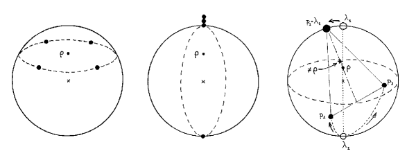
Figure 1: To the left we see a uniform distribution with $N=4$ for the density matrix ${\rho}=\mbox{diag}(3/4,1/4)$ in the Bloch ball and in the middle the degenerate uniform distribution that one would obtain from Nielsen’s procedure. By studying the rightmost picture one can convince oneself that if $p_{1}={\lambda}_{1}$ then any ensemble with $N>2$ pure states must be degenerate.

Clearly there are many ways to realize a uniform ensemble. Nielsen [5] provides a different procedure that relies on the theorem by Horn [6], discussed in the next section. Horn’s theorem tells us how to construct a matrix $U$ that obeys eq. (5) whenever $\vec{p}$ is majorized by $\vec{\lambda}$. This matrix is then used in eq. (3). But there is no guarantee that the states $|{\psi}_{i}\rangle$ are distinct. Explicit calculation shows that generically they are not, except when $N=M$. What this shows is that Theorem 1 must be used with some care. While the rows of a unitary matrix are never equal, it may still be true that the first $M$ components of a pair of rows in a unitary $N\times N$ matrix coincide. If this happens two of the pure states in the decomposition (2) will coincide too, and the ensemble will in fact not be uniform (see fig. 1). An analogous difficulty affects non-uniform ensembles as well. More details will be provided in section 4, once we have sketched some relevant background.

Further inspection of the Bloch ball reveals that Conjecture 1 cannot be true in general. It obviously fails for pure states. A more interesting counterexample is the following: Let $({\lambda}_{1},{\lambda}_{2})=(1/2,1/2)$. This is the maximally mixed state. Let $(p_{1},p_{2},p_{3})=(\frac{1}{2},\frac{1}{4},\frac{1}{4})$. Clearly $\vec{p}\prec\vec{\lambda}$. But it is geometrically evident that an ensemble of pure states with these $p_{i}$ as probabilities cannot give the maximally mixed state: Our three states define a plane through the Bloch ball that has to go through the center of the ball (where the maximally mixed state sits). The convex sum of the two states with probability $1/4$ lies inside the ball and the density matrix must lie on the straight line between that point and that of the state with probability $1/2$. But then the density matrix cannot lie in the center of the ball as stated. An extension of this argument shows that when $M=2$ it is always impossible to realize a non-degenerate ensemble with $p_{1}={\lambda}_{1}$ and $N>2$. See fig. 1.

3. Majorization and bistochastic matrices.

To bring the issues into focus a review of the mathematical background is called for. Majorization, as defined in the introduction, provides a natural partial preordering of vectors, and in particular of discrete probability distributions (positive vectors with trace norm equal to one). It is a preordering because $\vec{p}\prec\vec{q}$ and $\vec{q}\prec\vec{p}$ does not imply $\vec{p}=\vec{q}$, only that the vector $\vec{q}$ is obtained by permuting the components of $\vec{p}$. The notion is important in many contexts, ranging from economics to LOCC (Local Operations and Classical Communication) of entangled states in quantum mechanics [7].

The set of probability vectors is a convex simplex, and the set of such vectors that are majorized by a given vector forms a convex polytope with its corners at the $N!$ vectors obtained by permuting the $N$ components of the given vector. It is helpful to keep the simplest example in mind. Let the number of components be $N=3$. Then the set forms a triangle, and the set of vectors majorized by a given vector is easily recognized (see fig. 2).

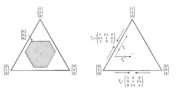
Figure 2: The probability simplex for $N=3$. To the left we see the set of vectors majorized by a given vector sitting in the corner of the shaded polytope. To the right we see how to get from one probability vector to another by means of two $T$–transforms.

A basic fact about majorization is a theorem due to Hardy, Littlewood and Pólya, that states that $\vec{p}\prec\vec{q}$ if and only if there exists a bistochastic matrix $B$ such that $\vec{p}=B\vec{q}$. A stochastic matrix is a matrix with non–negative entries such that the elements in each column sum to unity, which means that the matrix transforms probability vectors to probability vectors. It is bistochastic if also its rows sum to unity, which means that the uniform distribution $\vec{e}=\frac{1}{N}(1,1,\ ...\ ,1)$ is a fixed point of the map. According to Birkhoff’s theorem the space of bistochastic $N$ by $N$ matrices is an $(N-1)^{2}$ dimensional convex polytope with the $N!$ permutation matrices making up its corners. In the center of the polytope we find the van der Waerden matrix $B_{*}$ all of whose entries are equal to $1/N$.

Some special cases of bistochastic matrices will be of interest below. A $T$–transform is a bistochastic matrix that acts non-trivially only on two entries of the vectors. By means of permutations it can therefore be brought to the form

$$T=\left(\begin{array}[]{ccccc}t&1-t&0&\cdots&0\\ 1-t&t&0&\cdots&0\\ 0&0&1&\cdots&0\\ \vdots&\vdots&\vdots&\ddots&\vdots\\ 0&0&0&\cdots&1\end{array}\right)\ ,\hskip 14.22636pt0\leq t\leq 1\ .$$ (9)

Given two vectors $\vec{p}\prec\vec{q}$ there always exists a sequence of $N-1$ $T$–transforms such that $\vec{p}=T_{N-1}\ ...\ T_{1}\vec{q}$. On the other hand (except when $N=2$) it is not true that every bistochastic matrix can be written as a sequence of $T$–transforms. Fig. 2 shows how $T$–transforms act when $N=3$.

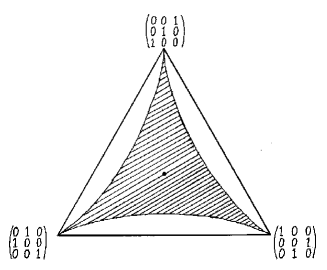
Figure 3: A two dimensional slice through Birkhoff’s polytope; the shaded region consists of unistochastic matrices and the dot in the center represents the van der Waerden matrix. Some interesting observations are made about it in ref. [9], where a closely related picture is drawn.

Unistochastic matrices were defined in the introduction. An orthostochastic matrix is a special case of that where the matrix elements of the bistochastic matrix are given by squares of the corresponding element of an orthogonal matrix. Horn’s theorem [6] states that given $\vec{p}\prec\vec{q}$ one can always find an orthostochastic matrix $B$ such that $\vec{p}=B\vec{q}$. The proof is by induction and actually gives a construction of $B$ as a sequence of $N-1$ $T$–transforms. The set of unistochastic matrices form a compact connected subset of the set of bistochastic matrices. When $N>2$ not all bistochastic matrices are unistochastic (see fig. 3). The van der Waerden matrix is unistochastic. It will be of interest below to know that sequences of $T$–transforms are always unistochastic when $N=3$, but that this is not so when $N>3$ [8]. For a more extensive discussion of unistochastic matrices we recommend reference [9].

4. Conjectures.

We can now return to the question of precisely which probability vectors $\vec{p}$ that can occur in non-degenerate ensembles for a density matrix with eigenvalue vector $\vec{\lambda}$. We know that $\vec{p}\prec\vec{\lambda}$. Nielsen’s idea [5] is to rely on Horn’s theorem to provide an orthostochastic matrix $B$ connecting the two vectors. The catch—from our point of view—is that the resulting ensemble will be degenerate in generic cases.

In section 2 we pointed out a class of counterexamples to Conjecture 1 for two dimensional Hilbert spaces. We can now see in a different way how they arise for arbitrary dimension $N$. Let

$$p_{1}+\ ...\ +p_{k-1}={\lambda}_{1}+\ ...\ +{\lambda}_{k-1}$$ (10)

and assume ${\lambda}_{k-1}>{\lambda}_{k}$. It is then easy to show that any bistochastic matrix connecting the two vectors must take the block diagonal form

$$B=\left(\begin{array}[]{cc}D_{1}&0\\ 0&D_{2}\end{array}\right)\ ,$$ (11)

where $D_{1}$ and $D_{2}$ are bistochastic matrices in themselves. $D_{1}$ is a $(k-1)\times(k-1)$ matrix. If $k=M$ then the form of $B$ means that only one column of $D_{2}$ is actually used in constructing no less than $N-M+1$ of the pure states in eq. (3), so that all these state vectors are contained in a one dimensional subspace. Hence the ensemble must have at least that degree of degeneracy, for essentially the same reason that a pure density matrix leads to a totally degenerate ensemble. It is tempting to guess that this is the only kind of counterexample to Conjecture 1 that can arise. Note however that the geometric argument in section 2 was actually a little more general as far as the case $M=2$ is concerned, and excludes also the case ${\lambda}_{M-1}={\lambda}_{M}$.

When $k<M$ in eq. (10) there is no obvious reason why the block diagonal form of $B$ must lead to degeneracies, and in fact this is not so in the (few) examples that we checked. In the concluding section we will conjecture that we have already found all the necessary additional restrictions that are missing from Conjecture 1.

Let us approach the problem from another direction. Given $\vec{p}\prec\vec{\lambda}$ can we find an algorithm for how to construct a unistochastic matrix $B$ such that $\vec{p}=B\vec{\lambda}$ and such that the corresponding unitary matrix leads to a non-degenerate ensemble? To begin with let us assume that $\vec{p}=\vec{e}$ and let us ask for a sequence of $T$–transforms that produces the “natural” uniform ensemble presented in section 2. An algorithm that does this is to first apply a $T$–transform $T_{1}$ with $t=1/2$ to the first two entries in $\vec{p}$, then a $T$-transform $T_{2}$ with $t=1/2$ to the second and third entries, and so on until $T_{N-1}$ sets the last two components of the vector equal. Then we repeat the procedure an infinite number of times. We get

$$\lim_{n\rightarrow\infty}(T_{N-1}T_{N-2}\ ...\ T_{1})^{n}=\frac{1}{N}\left(\begin{array}[]{ccccc}1&1&1&\cdots&1\\ 1&1&1&\cdots&1\\ 1&1&1&\cdots&1\\ \vdots&\vdots&\vdots&\ddots&\vdots\\ 1&1&1&\cdots&1\end{array}\right)\ .$$ (12)

This is the van der Waerden matrix $B_{*}$ which is unistochastic and when used in Schrödinger’s theorem does in fact lead to the natural uniform ensemble from section 2. To see that the sequence converges to $B_{*}$ we simply observe that the $T$–transforms do not depend on the vector $\vec{p}$ that we start out with. Therefore we can read off the columns of $B_{*}$ by seeing how it acts on the corners of the probability simplex, that is the vectors $(1,0,\ ...\ ,0)$ and so on.

Clearly this algorithm can be generalized to arbitrary $\vec{p}$ and $\vec{\lambda}$. The key idea is to choose, at each step, a $T$–transform that ensures the equality $p_{k}/p_{k-1}={\lambda}_{k}/{\lambda}_{k-1}$. Typically this will again converge to a definite bistochastic matrix $B$ in an infinite number of steps, this time because the individual $T$–transforms approach the unit matrix. In the examples that we checked (mostly for three-by-three matrices) it does produce a non-degenerate ensemble except for the counterexamples we already have. We therefore have a candidate for a constructive algorithm with the desired properties.

Unfortunately we do not know if the candidate is good enough. We do not know that it always results in a unistochastic matrix, let alone a non-degenerate ensemble. Already the first question becomes non-trivial when $N>3$, as noted in section 3. What we do know is that a sequence of $T$–transforms always meets the “chain-links” conditions from ref. [10] (see also [9]). These are necessary but not sufficient conditions that a bistochastic matrix is unistochastic. The idea is as follows: Take a bistochastic matrix

$$B=\left(\begin{array}[]{ccc}a_{1}&b_{1}&c_{1}\\ a_{2}&b_{2}&c_{2}\\ a_{3}&b_{3}&c_{3}\end{array}\right)\ .$$ (13)

Form the “links” $L_{i}=\sqrt{a_{i}b_{i}}$. If $B$ is unistochastic it must be true that

$$L_{1}\leq L_{2}+L_{3}\ ,\hskip 8.53581ptL_{2}\leq L_{3}+L_{1}\hskip 8.53581pt\mbox{and}\hskip 8.53581ptL_{3}\leq L_{1}+L_{2}\ .$$ (14)

These are called the chain-links conditions (stated in terms of columns) because they make it possible to form a “chain” (in this case a triangle) out of the links. This in turn ensures that a set of phases ${\mu}_{1}$, ${\mu}_{2}$ can be found such that the matrix

$$\left(\begin{array}[]{lll}\sqrt{a_{1}}&\sqrt{b_{1}}&\cdot\\ \sqrt{a_{2}}&\sqrt{b_{2}}e^{i{\mu}_{1}}&\cdot\\ \sqrt{a_{3}}&\sqrt{b_{3}}e^{i{\mu}_{2}}&\cdot\end{array}\right)$$ (15)

is unitary. (It is unnecessary to check the last column.) For three by three matrices the chain-links conditions are sufficient. For $N$ by $N$ matrices with $N>3$ the story becomes more complicated. The chain-links conditions still state that no one of the lengths (constructed analogously) can be larger than the sum of all the others. When one tries to construct the unitary matrix the number of equations to solve is the same as the number of phases available, but it can happen that the equations have no solution. Therefore the chain-links conditions are necessary but not sufficient when $N>3$.

Lemma: A sequence of $T$–transforms always obeys the chain-links conditions.

Sketch of proof: A single $T$–transform is unistochastic. Consider any sequence of $T$–transforms. Suppose that the first $n$ of these form a matrix $B$ that obeys the chain-links conditions. It is enough to prove that this implies that $TB$ obeys the chain-links conditions, where $T$ is any $T$–transform. (Since the set of matrices that obey these conditions is compact, infinite sequences pose no particular problem.) Consider therefore

$$T(t)B=\left(\begin{array}[]{ccc}1&0&0\\ 0&t&1-t\\ 0&1-t&t\end{array}\right)\left(\begin{array}[]{ccc}a_{1}&b_{1}&\cdot\\ a_{2}&b_{2}&\cdot\\ a_{3}&b_{3}&\cdot\end{array}\right)\ ,\hskip 14.22636pt0\leq t\leq 1\ .$$ (16)

With the links $L_{i}(t)$ formed from the matrix $T(t)B$ as indicated above, we must show that

$$L_{1}(1)\leq L_{2}(1)+L_{3}(1)\hskip 14.22636pt\Rightarrow\hskip 14.22636ptL_{1}(t)\leq L_{2}(t)+L_{3}(t)\ .$$ (17)

(Note that $T(1)B=B$ which obeys the conditions by assumption.) Since $L_{1}(t)$ is constant it is enough to verify that the function $L_{2}(t)+L_{3}(t)$ is larger than $L_{2}(1)+L_{3}(t)$ everywhere in the interval. We observe that this function is symmetric around $t=1/2$ and a straightforward calculation verifies that it assumes its only extremum there, and that this extremum is a maximum. The proof that the other chain-links conditions hold is similar. Extension of the proof to larger matrices and to the chain-links condition stated in terms of rows rather than columns is also straightforward.

For three-by-three matrices this establishes the result of ref. [8], that any sequence of $T$–transforms is unistochastic. For larger matrices the chain-links condition is necessary but not sufficient for that and there do exist sequences of $T$–transforms that are not unistochastic. It remains possible that the particular kind of sequence that we propose as an algorithm to realize an ensemble with probability vector $\vec{p}$ always results in unistochastic matrices but we have failed to prove this. Assuming that this can be done we would still have to prove that the ensemble that results from the unitary matrix so constructed is non-degenerate for all allowed probability vectors. This appears to be significantly more difficult.

5. Conclusions.

We have studied the question of precisely what kind of discrete probability distributions that can appear in an ensemble of pure states that describe a given density matrix. Evidently our main conclusion is that this question has more facets to it than one might suspect based on earlier literature [5]. We think that one answer is the following:

Conjecture 2: Given any probability vector $\vec{p}$ majorized by the eigenvalue vector $\vec{\lambda}$. Assume that the density matrix is not pure. Then there exists a set of distinct pure states $|\psi_{i}\rangle$ such that eq. (2) holds if and only if $p_{1}+\ ...\ +p_{M-1}\neq{\lambda}_{1}+\ ...\ +{\lambda}_{M-1}$.

The “only if” part of the statement is proved for $M=2$. For $M>2$ the case ${\lambda}_{M-1}={\lambda}_{M}$ may need separate attention, otherwise the “only if” part is again proved. The “if” part is only weakly supported by arguments and examples.

We also made a suggestion for how, given a $\vec{p}$ consistent with Conjecture 2, one might go about to construct such an ensemble by means of a sequence of $T$–transforms, but this suggestion is very weakly supported. Essentially the only argument is that the procedure does give the geometrically natural uniform ensemble when $\vec{p}=\vec{e}$.

Acknowledgement:

We thank Göran Lindblad, Wojciech Słomczyński and Karol Życzkowski for discussions and help; also an anonymous referee for comments.

References

- [1] E. Schrödinger, Proc. Camb. Phil. Soc. 32 (1936) 446.
- [2] L. P. Hughston, R. Josza and W. K. Wootters, Phys. Lett. A183 (1993) 14.
- [3] T. Ando, Lin. Alg. Appl. 118 (1989) 163.
- [4] A. Uhlmann, Rep. Math. Phys. 1 (1970) 147.
- [5] M. A. Nielsen, Phys. Rev. A62 (2000) 052308.
- [6] A. Horn, Amer. J. Math. 76 (1954) 620.
- [7] M. A. Nielsen, Phys. Rev. Lett. 83 (1999) 436.
- [8] Y.-T. Poon and N.-K. Tsing, Lin. Multilin. Alg. 21 (1987) 253.
- [9] K. Życzkowski, M. Kuś, W. Słomczyński and H.-J. Sommers, Random unistochastic matrices, arXiv preprint nlin.CD/ 0112036.
- [10] P. Pakoński, K. Życzkowski and M. Kuś, J. Phys. A34 (2001) 9303.