Quantum Zeno effect in a model multilevel molecule

Abstract

We study the dynamics of the populations of a model molecule endowed with two sets of rotational levels of different parity, whose ground levels are energy degenerate and coupled by a constant interaction. The relaxation rate from one set of levels to the other one has an interesting dependence on the average collision frequency of the molecules in the gas. This is interpreted as a quantum Zeno effect due to the decoherence effects provoked by the molecular collisions.

CNR-IMIP] Istituto di Metodologie Inorganiche e dei Plasmi, Consiglio Nazionale delle Ricerche, Bari, Italy Università di Bari-Matematica] Dipartimento di Matematica, Università di Bari, Bari, Italy [INFN-Bari] Istituto Nazionale di Fisica Nucleare, Sezione di Bari, Bari, Italy Università di Bari-Chimica] Dipartimento di Chimica, Università di Bari, Bari, Italy [CNR-IMIP] Istituto di Metodologie Inorganiche e dei Plasmi, Consiglio Nazionale delle Ricerche, Bari, Italy CNR-IMIP] Istituto di Metodologie Inorganiche e dei Plasmi, Consiglio Nazionale delle Ricerche, Bari, Italy Università di Bari-Fisica] Dipartimento di Fisica, Università di Bari, Bari, Italy [INFN-Bari] Istituto Nazionale di Fisica Nucleare, Sezione di Bari, Bari, Italy ICTP] Abdus Salam International Centre for Theoretical Physics, Trieste, Italy [INFN-Trieste] Istituto Nazionale di Fisica Nucleare, Sezione di Trieste, Trieste, Italy

1 Introduction

The quantum Zeno effect is usually formulated as the hindrance of the evolution of a quantum system due to frequent measurements performed by a classical apparatus ^{1, 2} and is formalized according to von Neumann projection rule ³. The literature of the last few years on this topic is vast and contemplates a variety of physical phenomena, ranging from oscillating (few level) systems ⁴ and alternative proposals ⁵ to bona fide unstable systems ⁶, where the so-called ”inverse” Zeno effect can take place.

The ideas and concepts at the basis of the quantum Zeno effect (QZE) were also successfully extended to continuous measurement processes by different authors and in different contexts ⁷ and led to a remarkable explanation of the stability of chiral molecules ⁸. This was a fertile idea, in that it explained the behavior of a variety of physical systems in terms of a similar underlying mechanism.

The QZE is, however, a much more general phenomenon, that takes place when a quantum system is strongly coupled to another system ⁹ or when it undergoes a rapid dephasing process. Such a rapid loss of phase coherence (”decoherence”) of the quantum mechanical wave function (for instance as a result of frequent interactions with the environment) is basically equivalent to a continuous measurement process (the main difference being that the state of the system is not necessarily explicitly recorded by a pointer).

The quantum Zeno effect is always ultimately ascribable to the short-time features of the dynamical evolution law ¹⁰: it is only the study of this dynamical problem that determines the range in which a frequent disturbance or interaction will yield a QZE. The very definition of ”frequent” is a delicate problem, that depends on the features of the interaction Hamiltonian. Moreover, one should also notice that the quantum system is not necessarily frozen in its initial state ¹¹, but rather undergoes a ”quantum Zeno dynamics”, possibly evolving away from its initial state ¹³. The study of such an evolution in the ”quantum Zeno subspace” ¹² is in itself an interesting problem, whose mathematical and physical aspects, as well as the possible applications to chemistry and physical chemistry, are not completely clear and require further study and elucidation.

After the seminal experiment by Itano and collaborators ⁴, the QZE has been experimentally verified in a variety of different situations, on experiments involving photon polarization ¹⁴, nuclear spin isomers ¹⁵, individual ions ^{16, 17, 18, 19}, optical pumping ²⁰, NMR ²¹, Bose-Einstein condensates ²², the photon number of the electromagnetic field in a cavity ²³, and new experiments are in preparation with neutron spin ^{24, 25}.

We focus here on the interesting example of QZE proposed in ¹⁵: the nuclear spin depolarization mechanisms in ¹³CH₃F, due to magnetic dipole interactions and collisions among the molecules in the gas, was experimentally investigated and interpreted as a QZE. In a few words, the ¹³CH₃F molecule has two kinds of angular momentum states, according to the value of the total spin of the three protons (H nuclei): $I=3/2$ (ortho) and $I=1/2$ (para). Transitions between states with different parity are (electric dipole) forbidden, so that spin flip occurs via a weak coupling between two levels of different spin parity (this is most effective when there is an accidental degeneracy between the levels, achievable, for example, via a Stark effect ²⁶). One observes a significant dependence of the spin relaxation on the gas pressure and interprets this as a QZE provoked by the dephasing due to molecular collisions. Nuclear spin conversion in polyatomic molecules is reviewed in ²⁷.

The aim of this article is to study the occurrence of the QZE in the general framework of collision-inhibited Rabi-like oscillations between two sets of rotational levels. We shall study the evolution of the level populations in a model multilevel molecule endowed with two sets of rotational levels of different parity. In particular, we shall concentrate on the interesting effects that arise as a consequence of the interactions (collisions) with the other molecules in the gas. The model we shall adopt will be studied both numerically and analytically, and the results will be compared. One of the main objectives of our investigation will be the analysis of apparently different phenomena in terms of a Zeno dynamics.

We shall introduce the system in Section 2 and the Zeno problem in the present context in Section 3. In Sections 4-6 we study the problem from an analytic point of view, by deriving and approximately solving a master equation. In Section 7 the analytical result are compared to an accurate numerical simulation. We conclude in Section 8 with a few remarks.

2 The system

Our model molecule has two subsets of rotational levels (to be called left ($L$) and right ($R$) levels in the following) of different parity, whose ground levels are energy degenerate and coupled by a constant interaction. (The choice of the ground levels is motivated by simplicity: one could choose any other couple of energy-degenerate levels in the $L$-$R$ subspaces.) The molecules undergo collisions with other identical molecules in the gas and we assume that these collisions couple the rotational energy levels but do not violate spin parity conservation. We shall focus on the dependence of the relaxation rate on the average collision time or, equivalently, on gas pressure: a QZE takes place if the transition between the left and right subspaces is inhibited when the collisions become more frequent (i.e., the gas pressure increases).

A sketch of the system is shown in 1.

Figure 1: Poissonian collisions in a gas of multilevel molecules.

The total Hilbert spaces of each molecule is made up of two subspaces ${\cal H}_{L}$ (left) and ${\cal H}_{R}$ (right), with $N_{L}$ and $N_{R}$ levels respectively. Collisions cannot provoke $L\leftrightarrow R$ transitions, so that no transitions are possible between the two subspaces, except through their ground states. However, collisions with other particles in the gas provoke transitions within each subspace.

The Hamiltonian is

$$H=H_{f}+H_{\mathrm{coll}}(t)=H_{0}+H_{1}+H_{\mathrm{coll}}(t),$$ (1)

where $H_{f}=H_{0}+H_{1}$ is the free Hamiltonian and

$$H_{0} = \sum_{n_{L}=1}^{N_{L}}E_{n_{L}}|n_{L}\rangle\langle n_{L}|+\sum_{n_{R}=1}^{N_{R}}E_{n_{R}}|n_{R}\rangle\langle n_{R}|,\$$ (2)

$$H_{1} = \hbar\Omega\left(|1_{L}\rangle\langle 1_{R}|+|1_{R}\rangle\langle 1_{L}|\right),$$ (3)

$$H_{\mathrm{coll}} = \hbar\sum_{j}\delta(t-\tau_{j})\;V,$$ (4)

$$V = \alpha_{L}V_{L}+\alpha_{R}V_{R},$$ (5)

$$V_{s} = \sum_{n_{s}=1}^{N_{s}-1}V_{n_{s}}=\sum_{n_{s}=1}^{N_{s}-1}|n_{s}\rangle\langle n_{s}+1|+|n_{s}+1\rangle\langle n_{s}|,\;\;\;\;$$ (6)

with $s=L,R$. The energy levels $|n_{s}\rangle$ have energies $E_{n_{s}}$ ($s=L,R$) and $H_{1}$ provokes $L\leftrightarrow R$ transitions between the two ground states, with (Rabi) frequency $\Omega$. $\Omega$ is small (in a sense to be made precise later), for such a transition is electric-dipole forbidden. $H_{\mathrm{coll}}$ accounts for the effect of collisions with the gas (environment): the collisions are distributed according to the Poisson statistics, appropriate for gas phase with short-range binary collisions, so that they occur at times

$$\tau_{j+1}=\tau_{j}+\delta\tau_{j},$$ (7)

where $\delta\tau_{j}$’s are independent random variables with distribution

$$p(\delta\tau_{j})=\frac{1}{\tau}\exp(-\delta\tau_{j}/\tau)$$ (8)

and (common) average $\tau$. The coupling constants $\alpha_{L,R}$ are in general different from each other and measure the ”effectiveness” of a collision. For the sake of simplicity we assume that collisions provoke transitions only between adjacent levels [$V_{s}$ in (6) involves only ”nearest neighbors” couplings]. We will assume, for concreteness, that the energy levels are rotational, so that

$$E_{n_{s}}=\hbar\omega_{s}n_{s}(n_{s}+1)\quad(s=L,R)$$ (9)

and $|1_{L}\rangle$ and $|1_{R}\rangle$ are the only resonant pair of states:

$$E_{1_{L}}=E_{1_{R}},\qquad E_{m_{L}}\neq E_{n_{R}}\quad\mbox{for}\quad m_{L},n_{R}>1.$$ (10)

See 1. The Hilbert spaces ${\cal H}_{L}$ and ${\cal H}_{R}$ are finite dimensional, with dimensions $N_{L}$ and $N_{R}$, respectively. This is because, in general, the number of accessible rotational levels is limited to a few tens, since for sufficiently high energies molecules tend to dissociate. This could be accounted for by introducing two ”absorbing” levels $|N_{L+1}\rangle,|N_{R+1}\rangle$ ²⁸. However, in our analysis, we will explore a time region in which the introduction of absorbing levels is not necessary (in other words, the times involved will not be long enough to display ”border effects”).

3 Zeno effect

Before we start our theoretical and numerical analysis it is convenient to focus on the physics of the model introduced in the preceding section and to clarify in which sense we expect a Zeno effect to take place. We start from a simple numerical experiment and calculate the time evolution of the populations by the Monte Carlo method described in²⁹.

Consider a uniform gas of identical molecules, having the internal structure described in the preceding section. A single molecule freely wanders in a total volume and undergoes random collisions. By neglecting the spatial component of the wave function, each molecule can be represented by an ($N_{L}+N_{R}$)-dimensional state vector $|\psi(t)\rangle$ that describes its internal state ³⁰. This physical situation is well schematized by the model described in Sec. 2. During the free flight the evolution is governed by the free hamiltonian

$$|\psi(t)\rangle=\exp\left(-\frac{i}{\hbar}H_{f}t\right)|\psi(0)\rangle.$$ (11)

Since the molecules are immersed in a bath, the collisions are distributed in time according to the Poisson statistics (7)-(8), with average collision frequency (per particle) $\tau^{-1}$. Once a collision occurs, a collision time is sampled according to:

$$\delta\tau=-\tau\log(y),$$ (12)

$y$ being a random number uniformly distributed in $[0,1[$. The collisions are modelled as instantaneous events and act on the left/right subspaces independently. As a result of a collision, the state becomes

$$|\psi(t+0^{+})\rangle=\exp\left(-i\sum_{s=L,R}\alpha_{s}V_{s}\right)|\psi(t)\rangle.$$ (13)

The matrix $\exp(-i\sum_{s}\alpha_{s}V_{s})$ is evaluated numerically. It is assumed to be independent of the internal state of the colliding partners and of their kinetic energy.

We also stress that since our aim is to investigate the occurrence of a QZE within the proposed level structure, we are not interested in the dissociation of highly excited molecules. To this end, we must restrict our attention to times such that the molecules do not ”see” the upper limit of the rotational levels, so that ”border” effects do not play any significant role. In this way the dissociation of highly excited molecules can be safely neglected.

The afore-mentioned qualitative features of our analysis will be carefully scrutinized and made precise in the following sections. We now take them for granted and give a few preliminary results in order to get a feeling for the physics at the basis of the Zeno effect.

We set $N_{L}=N_{R}=40$ energy levels, with energies given by (9), where $n_{s}=1,\dots,40$, $\omega_{L}=1.3\cdot 10^{10}\ {\mathrm{s}}^{-1}$ and $\omega_{R}=9.7\cdot 10^{9}{\mathrm{s}}^{-1}$. We always compute the average over an ensemble of $5\cdot 10^{3}$ particles. All particles are initially in the $|1_{L}\rangle$ state and we study the temporal behavior of the relative population in the left subspace

$$P_{L}\equiv\sum_{n_{L}}p_{n_{L}},$$ (14)

$p_{n_{L}}$ being the occupation probability of state $|n_{L}\rangle$.

The results of our numerical integration are shown in 2-3.

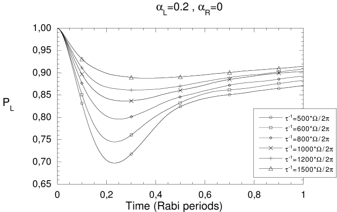
Figure 2: Temporal evolution of $P_{L}$. The collision frequency $\tau^{-1}$ is varied between $500T_{R}^{-1}$ and $1500T_{R}^{-1}$ ($T_{R}=2\pi/\Omega$). We set $\alpha_{L}=0.2,\alpha_{R}=0$, so that, in practice, $N_{L}=40$ left energy levels are coupled to only $N_{R}=1$ right level. The survival probability in the left subspace increases as the collision frequency is increased: frequent collisions hinder transition to the right subspace, a manifestation of a (”classically intuitive”) Zeno effect.

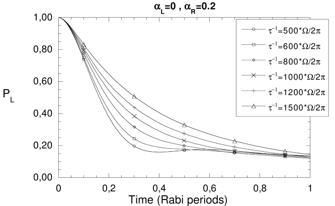
Figure 3: Temporal evolution of $P_{L}$. The collision frequency $\tau^{-1}$ is varied between $500T_{R}^{-1}$ and $1500T_{R}^{-1}$. Unlike in the previous figure, we set $\alpha_{L}=0,\alpha_{R}=0.2$, so that in practice, $N_{L}=1$ left level is coupled to $N_{R}=40$ right levels. Again, the survival probability in the left subspace increases as the collision frequency is increased: frequent collisions hinder transition to the right subspace, a manifestation of a (”classically counterintuitive”) Zeno effect.

In 2, $\alpha_{L}=0.2$ and $\alpha_{R}=0$, so that collisions do not provoke transitions among the right states (or, equivalently, the right subspace consists only of state $|1_{R}\rangle$). It is apparent that when the collision frequency $\tau^{-1}$ is increased between $500T_{R}^{-1}$ and $1500T_{R}^{-1}$ ($T_{R}=2\pi/\Omega$ being the Rabi period) the survival probability in the left subspace increases. If the collisions are viewed as a dephasing process (effectively yielding a ”measurement” of the occupation probabilities of the left states), this can be viewed as a Zeno effect. This is in agreement with our ”classical” intuition: since the system is initially in the left subspace and collisions remove population density from the ground state $|1_{L}\rangle$ of this subspace (the only level coupled to the right subspace), it is intuitively clear that, by increasing the collision frequency, transitions to the right subspace are hindered. This is a ”classically intuitive” version of the Zeno effect.

The situation depicted in 3 is different: here $\alpha_{L}=0$ and $\alpha_{R}=0.2$, so that now collisions do not provoke transitions among the left states, or equivalently the left subspace consists only of state $|1_{L}\rangle$ (which is also the only state coupled to the right subspace). Once again, when the collision frequency $\tau^{-1}$ is increased in the same range as before, the survival probability in the left subspace increases. We stress that the collisions are effective in hindering the transition from a single level towards a subspace that is initially empty. In other words, now the collisions act only on the right subspace, where virtually no particles are present. Once again, this can be viewed as a Zeno effect; however, it is somewhat less intuitive than the previous one (and maybe a bit puzzling for our ”classical” intuition). This a ”classically counterintuitive” version of the Zeno effect.

After having rapidly analyzed these two simple situations, we are ready to tackle the more general case of $N_{L}$ left levels coupled to $N_{R}$ right ones. This will be done in the following.

4 Master equation

4.1 The general case

We start our analysis by deriving a master equation for the density matrix of the molecule. Write (4) as

$$H_{\mathrm{coll}}(t)=\hbar\;\mu(t)V,$$ (15)

where

$$\mu(t)=\frac{dN(t)}{dt}=\sum_{j}\delta(t-\tau_{j})$$ (16)

is the derivative of a Poisson process $N(t)$ with mean time $\tau$ ³¹:

$$\mbox{Prob}\{N(t)=n\}=P(n,t)=e^{-t/\tau}\frac{1}{n!}\left(\frac{t}{\tau}\right)^{n}.$$ (17)

One gets

$$\langle dN(t)\rangle=\frac{dt}{\tau},\qquad\left\langle\left(dN(t)-\frac{dt}{\tau}\right)^{2}\right\rangle=\frac{dt}{\tau},$$ (18)

so that the process

$$dW(t)=\eta(t)dt=\mu(t)dt-\frac{dt}{\tau}=dN(t)-\frac{dt}{\tau}$$ (19)

has a vanishing mean and a linear variance in $dt$

$$\langle dW(t)\rangle=0,\qquad\left\langle dW(t)^{2}\right\rangle=\frac{dt}{\tau}.$$ (20)

In terms of the white noise $\eta(t)$ these equations read

$$\langle\eta(t)\rangle=0,\qquad\left\langle\eta(t)\eta(t^{\prime})\right\rangle=\frac{1}{\tau}\delta(t-t^{\prime}).$$ (21)

The collision Hamiltonian can then be rewritten in terms of a constant part and a white noise

$$H_{\mathrm{coll}}(t)=\frac{\hbar}{\tau}V+\hbar\;\eta(t)V,$$ (22)

whence the total Hamiltonian (1) reads

$$H=\bar{H}+\hbar\;\eta(t)V,\qquad\bar{H}=H_{0}+H_{1}+\frac{\hbar}{\tau}V.$$ (23)

The Schrödinger equation (in Itô form) is

$$|\psi(t+dt)\rangle=\left(1-\frac{i}{\hbar}\bar{H}dt-\frac{1}{2\tau}V^{2}dt\right)|\psi(t)\rangle-iVdW|\psi(t)\rangle$$ (24)

and the average density matrix [$\langle\cdots\rangle$ is introduced in Eq. (18)],

$$\rho(t)=\left\langle\;|\psi(t)\rangle\langle\psi(t)|\;\right\rangle,$$ (25)

follows a master equation in the Kossakowski-Lindblad form ³²

$$\frac{d\rho}{dt} = -\frac{i}{\hbar}\;[\bar{H},\rho]-\frac{1}{2\tau}\;[V,[V,\rho]]$$ (26)

$$= -\frac{i}{\hbar}\;[\bar{H},\rho]-\frac{1}{2\tau}\;\{V^{2},\rho\}+\frac{1}{\tau}\;V\rho V.$$

By using Eqs. (23), (5) and (6) we get

$$\frac{d\rho}{dt} = -\frac{i}{\hbar}\;[H_{0},\rho]-\frac{i}{\hbar}\;[H_{1},\rho]-\frac{i}{\tau}\;[V,\rho]-\frac{1}{2\tau}\;\{V^{2},\rho\}+\frac{1}{\tau}\;V\rho V$$ (27)

$$= -\frac{i}{\hbar}\;[H_{0},\rho]-\frac{i}{\hbar}\;[H_{1},\rho]+\sum_{s=L,R}\left(-i\frac{\alpha_{s}}{\tau}[V_{s},\rho]-\frac{\alpha_{s}^{2}}{2\tau}\{V_{s}^{2},\rho\}+\frac{\alpha_{s}^{2}}{\tau}V_{s}\rho V_{s}\right)$$

$$+\frac{\alpha_{L}\alpha_{R}}{\tau}\left(V_{L}\rho V_{R}+V_{R}\rho V_{L}\right).$$

This equation for the average density matrix (25) is exact, but complicated. However, it can be greatly simplified under some reasonable hypotheses.

4.2 Reduced master equation

We assume that all level pairs $E_{m_{R}}$ and $E_{n_{L}}$ are sufficiently far from resonance, namely

$$\frac{\Delta E}{\hbar}\gg\Omega,\ \tau^{-1},$$ (28)

where $\Delta E$ is the smallest energy difference between states $|m_{R}\rangle$ and $|n_{L}\rangle$, with $m_{R},n_{L}>1$. This requirement will be discussed in more detail in Section 7. At this stage we only observe that, typically, $\Delta E/\hbar\simeq 10^{-9}$s, while $\Omega\simeq 1$kHz and $\tau\simeq 1\mu$s, so the above condition appears very reasonable.

It is then possible to show that in (27) the dynamics of the populations $p_{m_{s}}=\rho_{m_{s}m_{s}}$ ($s=L,R$) plus the coherence term $\rho_{1_{L}1_{R}}$ completely decouples from the dynamics of the coherence terms $\rho_{m_{s}n_{s^{\prime}}}$ ($s,s^{\prime}=L,R$ and $m_{s},n_{s^{\prime}}\neq 1$). This is because, roughly speaking, no ”diagonal” fast frequency is present [essentially because $\langle m_{s}|[H_{0},\rho]|m_{s}\rangle=0$ in (27)] and, under hypothesis (28), the contribution of all the other fast terms is averaged to zero over the long timescales $\tau$ and $\Omega^{-1}$, and the dynamics of the slow and fast terms completely decouples. In conclusion, only the ”slow” dynamics is relevant over the large timescales $\tau$ and $\Omega^{-1}$.

The above argument has a general rigorous justification ¹² in terms of an adiabatic theorem and is elucidated in Appendix 9 for the model studied in this article. One shows that the part of the master equation (27) pertaining to the populations becomes

$$\frac{d\tilde{\rho}}{dt}\simeq-\frac{i}{\hbar}\;[\tilde{H}_{1},\tilde{\rho}]-\frac{i}{\tau}\;[\tilde{V},\tilde{\rho}]-\frac{1}{2\tau}\;\{\widetilde{V^{2}},\tilde{\rho}\}+\frac{1}{\tau}\;\widetilde{V\tilde{\rho}V},$$ (29)

where the reduced operator $\tilde{A}$, defined by

$$\tilde{A}=QAQ+\sum_{s=L,R}\sum_{m_{s}=2}^{N_{s}}P_{m_{s}}AP_{m_{s}},$$ (30)

involves only matrix elements belonging to the eigenspaces of $H_{0}$ ¹²,

$$Q=P_{1_{L}}+P_{1_{R}}\qquad\mbox{and}\quad P_{m_{s}}=|m_{s}\rangle\langle m_{s}|,$$ (31)

[remember condition (10)] and is diagonal with respect to $H_{0}$

$$[H_{0},\tilde{A}]=0.$$ (32)

In particular, from Eq. (3)

$$\tilde{H}_{1} = QH_{1}Q=H_{1}=\hbar\Omega\sigma_{1},$$

$$\sigma_{1} \equiv |1_{L}\rangle\langle 1_{R}|+|1_{R}\rangle\langle 1_{L}|$$ (33)

and from Eqs. (5) and (6)

$$\tilde{V}=0,\qquad\widetilde{V^{2}}=\sum_{s=L,R}\alpha_{s}^{2}\widetilde{V_{s}^{2}}=\sum_{s=L,R}\alpha_{s}^{2}\sum_{m_{s}=1}^{N_{s}-1}V_{m_{s}}^{2}$$ (34)

and

$$\widetilde{V\tilde{\rho}V}=\sum_{s=L,R}\alpha_{s}^{2}\widetilde{V_{s}\tilde{\rho}V_{s}}=\sum_{s=L,R}\alpha_{s}^{2}\sum_{m_{s}=1}^{N_{s}-1}V_{m_{s}}\tilde{\rho}V_{ms},$$ (35)

so that Eq. (29) reads

$$\frac{d\tilde{\rho}}{dt}=-i\Omega[\sigma_{1},\tilde{\rho}]-\sum_{s=L,R}\frac{\alpha_{s}^{2}}{2\tau}\sum_{m_{s}=1}^{N_{s}-1}[V_{m_{s}},[V_{m_{s}},\tilde{\rho}]].$$ (36)

This is the master equation we will study in detail. The only assumption made in its derivation is (28).

The reduced density matrix $\tilde{\rho}$ is given by Eq. (30) and involves only the level populations $p_{n_{s}}=\rho_{n_{s}n_{s}}$ ($s=L,R$) and the two coherence terms $\rho_{1_{L},1_{R}}$ and $\rho_{1_{R},1_{L}}$, all other matrix elements being zero. Thus, it describes two classical Markov chains $(1_{L},\ldots,N_{L})$ and $(1_{R},\ldots,N_{R})$, whose transition rates are proportional to $D_{L}=\alpha_{L}^{2}/\tau$ and $D_{R}=\alpha_{R}^{2}/\tau$ respectively, linked by quantum Rabi oscillations between $|1_{L}\rangle$ and $|1_{R}\rangle$, whose period is $T_{R}=2\pi/\Omega$.

By setting $D=(D_{L}+D_{R})/2$, i.e. $\alpha^{2}=(\alpha^{2}_{L}+\alpha^{2}_{R})/2$, the ratio between the two timescales

$$x=DT_{R}=\frac{\alpha^{2}}{\tau}T_{R}=\frac{2\pi\alpha^{2}}{\tau\Omega}$$ (37)

is an important parameter, that describes different dynamical regimes. Larger values of $x$ correspond to more frequent collisions (within a Rabi period) and consequently to a more evident manifestation of the QZE.

5 Stochastic dynamics in decoupled subspaces

Let us first study the subdynamics of each subspace ${\cal H}_{L/R}$ separately. To this end, set $\Omega=0$ in Eq. (36): the time evolution is governed only by the collision dynamics, the right and left subspaces decouple and their subdynamics can be studied separately.

In terms of ($s=L,R$)

$$\mbox{\boldmath$p$}^{s}=\left(\rho_{1_{s}1_{s}},\ldots,\rho_{n_{s}n_{s},\ldots}\right)=\left(p_{1_{s}},\ldots,p_{n_{s}},\ldots\right),$$ (38)

Eq. (36) reduces to

$$\frac{d\mbox{\boldmath$p$}^{s}}{dt}=D_{s}W^{s}\mbox{\boldmath$p$}^{s},$$ (39)

where $W^{s}$ is the stochastic matrix

$$W^{s}=\left(\begin{array}[]{ccccc}-1&1&0&0&\dots\\ 1&-2&1&0&\dots\\ 0&1&-2&1&\dots\\ 0&0&1&-2&\dots\\ \vdots&\vdots&\vdots&\vdots&\ddots\\ \end{array}\right),\qquad(s=L,R)\ \$$ (40)

and

$$D_{s}=\frac{\alpha^{2}_{s}}{\tau}.$$ (41)

Note that $W^{s}$ is a real symmetric matrix with real eigenvalues and a complete set of eigenvectors.

The resulting dynamics is diffusive. Indeed, Eq. (39) explicitly reads

$$\dot{p}_{1_{s}} = D_{s}\left(-p_{1_{s}}+p_{2_{s}}\right),\qquad\qquad(\Omega=0)$$ (42)

$$\dot{p}_{n_{s}} = D_{s}\left(p_{n_{s}-1}-2p_{n_{s}}+p_{n_{s}+1}\right),\quad(n_{s}\geq 2)$$ (43)

which is nothing but a diffusion equation (dropping the suffix $s$)

$$\partial_{t}p_{n}(t)=D\,\triangle p_{n}(t),$$ (44)

where

$$\triangle\equiv\frac{1}{2}\left(\nabla^{+}\nabla^{-}+\nabla^{-}\nabla^{+}\right),$$ (45)

and

$$\nabla^{+}p_{n}=p_{n+1}-p_{n},\qquad\nabla^{-}p_{n}=p_{n}-p_{n-1}.$$ (46)

The boundary condition $\nabla^{-}p_{1}=0$ [see Eq. (42)] is imposed by introducing a supplementary state $n=0$, whose probability satisfies $p_{0}=p_{1}$ for every $t$. The evolution of the population is made up of two terms (both expressed in terms of the fundamental solution of the heat equation): each ”site” (level) gets a direct and a ”reflected” contribution from the boundary $n=1$:

$$p_{n}(t)=q_{n}(Dt)+q_{1-n}(Dt),$$ (47)

where $q_{n}(t)$ are the probabilities of the continuous-time symmetrical random walk engendered by the equations ³³

$$\dot{q}_{n}=q_{n-1}-2q_{n}+q_{n+1},\quad-\infty<n<\infty,$$ (48)

whose solution starting at $n=1$ for $t=0$ [i.e. $p_{n}(0)=\delta_{n1}$] reads

$$q_{n}(t)=e^{-2t}I_{|n-1|}(2t),$$ (49)

$I_{n}(t)$ being the modified Bessel function ³⁴. As is well known, for $t\to\infty$ and $n\to\infty$ with $n^{2}/t=$const, this yields

$$q_{n}(t)\sim\frac{1}{\sqrt{4\pi t}}\exp\left(-\frac{(n-1)^{2}}{4t}\right).$$ (50)

Note that the boundary condition is essential in assuring probability conservation,

$$\sum_{n=1}^{+\infty}p_{n}(t)=\sum_{n=-\infty}^{+\infty}q_{n}(Dt)=1,$$ (51)

for any $t$. The above equations are of general validity. In particular,

$$p_{1}(t)=e^{-2Dt}\left[I_{0}(2Dt)+I_{1}(2Dt)\right],$$ (52)

(and $p_{1}(0)=1$). It is also possible, by using the solution (47) and (49), to evaluate the mean and second moment

$$\mu(t) = \sum_{n=1}^{\infty}np_{n}(t),$$ (53)

$$\sigma^{2}(t) = \sum_{n=1}^{\infty}n^{2}p_{n}(t)\ .$$ (54)

Indeed, by using (48), one can obtain explicit differential equations involving these quantities, valid for any $t$,

$$\dot{\mu}(t) = Dp_{1}(t)=De^{-2Dt}\left[I_{0}(2Dt)+I_{1}(2Dt)\right],$$

$$\dot{\sigma^{2}}(t) = 2D+Dp_{1}(t),$$ (55)

whose integration gives

$$\mu(t) = \frac{1}{2}+\frac{1}{2}e^{-2Dt}\left[(1+4Dt)\,I_{0}(2Dt)+4Dt\,I_{1}(2Dt)\right],$$

$$\sigma^{2}(t) = 2Dt+\mu(t).$$ (57)

Let us also give, for completeness, the expression of $\mu$ and $\sigma$ for times $Dt\gg 1$ [but always $t\ll T_{\mathrm{d}}$, see Eq. (60) below]. From Eqs. (LABEL:eq:mut)-(57),

$$\mu(t) \sim \sqrt{\frac{4D}{\pi}t},$$

$$\sigma(t) \sim \sqrt{2Dt}.$$ (58)

In order to compare these results with those of the following sections, consider that

$$Dt=x\frac{t}{T_{R}},$$ (59)

where $T_{R}$ is the Rabi period and $x=x_{s}=\alpha_{s}^{2}T_{R}/\tau\;(s=1,2)$ is essentially the scaling parameter introduced in (37).

In reality, as we already emphasized, the number $N$ ($N_{L}$ or $N_{R}$) of accessible rotational levels is in fact finite, because the molecule dissociates after absorbing a sufficient amount of energy. In order to account for this process one can add an $(N+1)$th absorbing level (in each subspace). However, since we are interested in phenomena, such as the QZE, that can be brought to light within timescales shorter than the dissociation time, the introduction of an absorbing level is an unnecessary complication that can be easily avoided by restricting our attention to the relevant timescales. Let us therefore estimate the time scale at which dissociation occurs. If a molecule dissociates when it reaches level $N+1$, namely if only $N$ levels take part in the diffusion process, the ”dissociation” time reads

$$T_{\mathrm{d}}\simeq\frac{N^{2}}{D}=\frac{N^{2}\tau}{\alpha^{2}}=\frac{N^{2}}{x}T_{R}.$$ (60)

This is the time needed by the system, that starts in the ground level, in order to reach the uppermost level via the diffusive propagation engendered by the collision. This rough estimate of the ”dissociation” time can be improved: a better analysis yields $T_{\mathrm{d}}=N^{2}\tau/\pi^{2}\alpha^{2}$, which is roughly of the same order of magnitude.

In our analysis we will assume $N=40$. Within the numerical range of the parameters $\alpha$ and $\tau$ to be used in our simulation, the dissociation time $T_{\mathrm{d}}$ varies between $2$ and $12$ Rabi periods. In the following we will always remain well below this threshold.

6 Zeno effect in coupled subspaces

We have seen in Section 3 that when the $L$ and $R$ subspaces are coupled, namely when $\Omega\neq 0$, a QZE can be obtained by increasing the collision frequency. Indeed, as we will show, by increasing the collision frequency, the probability of remaining in the initial subspace decays more slowly. We also commented on the possibility of studying the Zeno dynamics in two different situations, one classically more intuitive and the other one less intuitive. These different names reflect the fact that the former case can be understood (at least qualitatively) by means of a classical Markov process, while the latter cannot. Both Zeno effects are contained in the master equation derived in Section 4 and are a consequence of the features of the collisions with the other molecules constituting the environment, or in other words, of the coupling constants of the interaction Hamiltonian $H_{\mathrm{coll}}$. The resulting dynamics will be numerically investigated in full generality in Section 7. However, before we show the results of the numerical simulation, let us discuss the main qualitative features of the dynamics without solving the complete master equation. This will be done in the present section with the help of some working hypotheses and will help us clarify some additional features of the Zeno effects.

When $\Omega\neq 0$ the two subspaces ${\cal H}_{L}$ and ${\cal H}_{R}$ are coupled through their ground states. The evolution is described by (43), supplemented by the following three equations

$$\dot{p}_{1_{L}} = D_{L}\left(-p_{1_{L}}+p_{2_{L}}\right)+\Omega p^{c}(t),$$ (61)

$$\dot{p}_{1_{R}} = D_{R}\left(-p_{1_{R}}+p_{2_{R}}\right)-\Omega p^{c}(t),$$ (62)

$$\dot{p}^{c}(t) = -\frac{D_{L}+D_{R}}{2}p^{c}(t)-2\Omega\left(p_{1_{L}}(t)-p_{1_{R}}(t)\right),\ \$$ (63)

where $p^{c}$ is the coherence term between states $|1_{L}\rangle$ and $|1_{R}\rangle$

$$p^{c}=-2\mathrm{Im}\rho_{1_{L}1_{R}}=i\left(\rho_{1_{L}1_{R}}-\rho_{1_{R}1_{L}}\right),$$ (64)

responsible for the coupling between the two subspaces. The total probabilities of being in the left and right subspaces read

$$P_{L}(t)=\sum_{n_{L}}p_{n_{L}}(t),\quad P_{R}(t)=\sum_{n_{R}}p_{n_{R}}(t),$$ (65)

respectively. The derivatives of these quantities are easily seen to be simply related to the coherence term:

$$\dot{P}_{L}(t)=\Omega p^{c}(t),\quad\dot{P}_{R}(t)=-\Omega p^{c}(t).$$ (66)

Notice that $\dot{P}_{L}+\dot{P}_{R}=0$ (conservation of particles number). Let our particles start in the left subspace at time $t=0$. Therefore the quantity of interest is $P_{L}$. One can obtain the evolution equation for $P_{L}(t)$ by eliminating $p^{c}$ by means of (63)

$$\ddot{P}_{L}+D\dot{P_{L}}+2\Omega^{2}\left(p_{1_{L}}-p_{1_{R}}\right)=0,$$ (67)

where we set $D\equiv(D_{L}+D_{R})/2$. This equation shows that the dynamics of $P_{L}$ is governed only by the population difference between the ground states, irrespectively of the population of the higher levels. This introduces an interesting picture of the dynamics, in which the Rabi oscillations act as a ”source” for the probability. The source drains particles from the left to the right subspace if $p_{1_{L}}>p_{1_{R}}$ and vice versa if $p_{1_{L}}<p_{1_{R}}$.

Our initial condition will always be $p_{1_{L}}(0)=1$: initial population in the ground state of the left subspace. For $t\ll 1/D\ll T_{R}=2\pi/\Omega$ (which is always true for our choice of parameters), we can set $p_{1_{L}}(t)=1+O(Dt)$ and $p_{1_{R}}(t)=O(Dt)$ and a power-series solution of (67), with initial conditions $P_{L}(0)=1,\ \dot{P}_{L}(0)=0$, yields

$$P_{L}(t)=1-\Omega^{2}t^{2}+o(\Omega^{2}t^{2}),$$ (68)

which shows that the quadratic region of the Rabi oscillation is not perturbed by the collisional dynamics (namely, does not depend on $\alpha$), even thought it extends up to times shorter than $1/D\ll T_{R}$. This result was to be expected ⁹ and is well observed in our numerical experiments, also for very high collision frequencies.

Equation (67) is exact, but it is not a closed equation for the total probability $P_{L}$. One needs the populations of the ground states in order to obtain $P_{L}$. We will therefore introduce an ansatz for the functional form of the populations of the ground states, valid for large values of the parameter $x$ defined in Eq. (37), which will enable us to get a closed equation for $P_{L}$. In addition we will also gain a deeper understanding of the Zeno phenomenon for this system. The ansatz consists in substituting for $p_{1_{L/R}}$ the solution (52), obtained for the decoupled subspaces ($\Omega=0$), normalized to $P_{L/R}$. This ”adiabatic” (Born-Oppenheimer-like) approximation relies upon the assumption that the time scale of the internal collisional dynamics is much faster than the Rabi one ($1/D\ll T_{R}$), so that particles are drained from the ground level and redistributed according to the uncoupled dynamics. The Rabi coupling simply accounts for the varying number of particles present in each subspace. This ansatz is translated into the equations

$$p_{1_{L}} = P_{L}(t)f_{L}(t),$$

$$p_{1_{R}} = P_{R}(t)f_{R}(t)=(1-P_{L})f_{R}(t),$$ (69)

where $f_{L/R}(t)$ are the population probabilities of the ground states given by the uncoupled dynamics (52)

$$f_{L/R}=e^{-2D_{L/R}t}\left[I_{0}(2D_{L/R}t)+I_{1}(2D_{L/R}t)\right].$$ (70)

Substituting in (67) we obtain

$$\ddot{P}_{L}+D\dot{P}_{L}+2\Omega^{2}\left(P_{L}(f_{L}+f_{R})-f_{R}\right)=0,$$ (71)

which is the equation of motion of a unit-mass, forced pendulum with varying frequency. The initial conditions are $P_{L}(0)=1,\;\dot{P_{L}}(0)=0$. It is easy to prove that if $f_{R}/(f_{L}+f_{R})$ tends to a well-defined limit and its first and second derivatives vanish when $t\to\infty$, there is a stable fixed point at $t=\infty$

$$P_{L}^{*}=\frac{f_{R}(t)}{f_{R}(t)+f_{L}(t)}\Bigg{|}_{t\to\infty}$$ (72)

and any solution will eventually reach this point. This feature of the population of the left subspace is always observed in the numerical solutions. An asymptotic analysis of the Bessel functions, performed with $1/D\ll t\ll T_{\mathrm{d}}$ shows that all these requirements are satisfied and an equilibrium distribution exists and is given by

$$P_{L}^{*}=\frac{1}{1+\sqrt{D_{R}/D_{L}}}=\frac{\alpha_{L}}{\alpha_{L}+\alpha_{R}}.$$ (73)

Let us see now how the Zeno effect emerges in this picture in three different cases.

6.1 Case $\alpha_{L}=\alpha_{R}=\alpha\neq 0$

The first case-study is obtained by setting $\alpha=\alpha_{L}=\alpha_{R}\neq 0$, so that the (collision dynamics in the) two subspaces are identical and $f_{L}(t)=f_{R}(t)\equiv f(t)$. We change the time variable from $t$ to the dimensionless $t/T_{R}=2\pi t/\Omega$ and set $x=DT_{R}=\alpha^{2}T_{R}/\tau=2\pi\alpha^{2}\tau/\Omega$, obtaining (the dot denotes now differentiation with respect to $t/T_{R}$)

$$\ddot{P}_{L}+x\dot{P}_{L}+8\pi^{2}f(t)(2P_{L}-1)=0,$$ (74)

where $f(t)$ is given by (70). Since $D_{L}=D_{R}$, according to (73), $P_{L}$ will eventually tend to $P_{L}^{*}=1/2$. However, we will see that the typical time scale $T_{\mathrm{relax}}$ of this relaxation process will increase with $x$ and this will be interpreted as a QZE.

The proposed analogy with a classical damped harmonic oscillator suggests that when $x\gg 1$ we get $\dot{P}_{L}\sim 1/x^{\alpha}$ and $\ddot{P}_{L}\sim 1/x^{2\alpha}$, with $\alpha>1$. Indeed, we will see that the solution satisfies this hypothesis with $\alpha=3/2$, so that the first term ($\ddot{P}_{L}\sim x^{-2\alpha}$) is negligible with respect to the second ($x\dot{P}_{L}\sim x^{1-\alpha}$) and the third one (both $f$ and $P_{L}$ are of order 1) and hence can be dropped from (74). Thus we are left with a first-order, separable differential equation whose solution is [here $P_{L}(0)=1$ but $\dot{P}_{L}(0)=O(1/x)$]

$$P_{L}(t) = \frac{1}{2}+\frac{1}{2}\exp\left[\frac{8\pi^{2}}{x^{2}}\Big{(}1-e^{-2xt}(1+4xt)\;I_{0}(2xt)\right.$$ (75)

$$\qquad\qquad\qquad\qquad\left.-e^{-2xt}4xt\;I_{1}(2xt)\Big{)}\right].$$

For $xt\gg 1$ we obtain a stretched exponential

$$P_{L}(t)\simeq\frac{1}{2}+\frac{1}{2}\exp\left[\frac{8\pi^{2}}{x^{2}}-32\pi^{3/2}\left(\frac{t}{x^{3}}\right)^{1/2}\right],$$ (76)

from which one can define a relaxation time as the only characteristic time present in the exponential (restoring natural time units):

$$T_{\mathrm{relax}}\propto x^{3}T_{R}.$$ (77)

The Zeno effect consists in the fact that by increasing $x$ (more frequent collisions) the corresponding curves of $P_{L}$ tend to zero more slowly. These predictions are in qualitative and quantitative agreement with the numerical simulations of the next section.

In order to get a rough preliminary idea of the issues discussed in this section, look for instance at 4 and 5, where the numerical results (to be described in greater details in the following) are compared to Eqs. (76)-(77). The probability (75)-(76) is correct up to a precision of $10\%$, showing that the ansatz (69) yields sensible results. Notice that $x=48$ in 4, so that the solution (76), which is supposed to be valid for $xt\gg 1$, must yields accurate results for $t/x^{3}\geq 10^{-6}$, as one indeed observes. A numerical fit for the exponent in the stretched-exponential yields $t^{0.3}$ rather than $t^{1/2}$, confirming the general functional dependence. The very fact that the global relaxation law is of the stretched-exponential type suggests that the dynamics is highly nontrivial, but we will not elaborate on this here. Finally, as can be seen from 5, the scaling law (77) is very well verified.

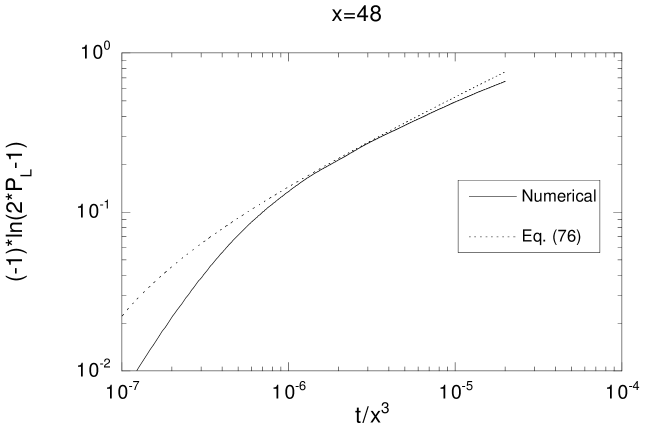
Figure 4: Comparison between the numerical results and Eq. (76). We set $x=48$.

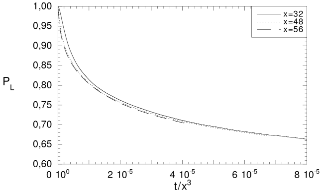
Figure 5: Rescaled probabilities for $x=32,\;48,\;56$ (numerical results).

6.2 Case $\alpha_{L}\neq\alpha_{R}=0$

Let us briefly reconsider the first case analyzed in Sec. 3, 2. Here the left subspace is affected by collisions while the right one is not. Although this is not a realistic situation, it is interesting and instructive to look at it. We shall show that also in this case, as the collision strength is increased, the system tends to spend more time in the initial (left) subspace.

If $\alpha_{R}=0$ and $\alpha_{L}\neq 0$ then $f_{L}\equiv f$ and $f_{R}=1$ and Eq. (71) reads

$$\ddot{P}_{L}+x\dot{P}_{L}+8\pi^{2}[P_{L}(1+f(t))-1]=0,$$ (78)

where $x=\alpha_{L}^{2}T_{R}/2\tau=\pi\alpha_{L}^{2}/\Omega\tau$. By means of the same approximations of the preceding subsection we obtain, for $x\gg 2\sqrt{2}\pi$,

$$P_{L}(t) \simeq 1-\frac{2\sqrt{2}\pi}{x}e^{-\left(\sqrt{\frac{8\pi^{2}t}{x}}+\frac{2\sqrt{2\pi}}{x}\right)^{2}}$$ (79)

$$\times\Phi\left(\sqrt{\frac{8\pi^{2}t}{x}}+\frac{2\sqrt{2\pi}}{x}\right),$$

where $\Phi(z)$ is the error function of imaginary argument ³⁴

$$\Phi(z)=\frac{2}{\sqrt{\pi}}\int_{0}^{z}dxe^{x^{2}}.$$ (80)

Here the definition of a relaxation time is not easy (no simple scaling law exists). However, both in this solution and in the numerical data, $P_{L}$ has a single minimum $P^{*}_{L}$, which is an increasing function of $x$: this can be regarded as a manifestation of a (classically intuitive) Zeno effect, as explained in Sec. 3. From (79) the value of the minimum is

$$P_{L}^{*}=1-\frac{2.7}{x}$$ (81)

and is an increasing function of $x$ . This law is well confirmed by the numerical results shown in 2. Beyond the minimum $P_{L}$ tends to 1 with a power-law

$$P_{L}(t)\simeq 1-\sqrt{\frac{4}{\pi xt}}\;.$$ (82)

This is again a Zeno effect: by increasing the collision rate $x$ the survival probability increases.

6.3 Case $\alpha_{R}\neq\alpha_{L}=0$

This is the second case analyzed in Sec. 3, 3. If $\alpha_{L}=0,\ \alpha_{R}\neq 0$, then $f_{R}=f,f_{L}=0$ and Eq. (71) reads (here $x=\alpha_{R}^{2}T_{R}/2\tau$)

$$\ddot{P}_{L}+x\dot{P}_{L}+8\pi^{2}[P_{L}(1+f(t))-f(t)]=0.$$ (83)

Again we neglect $\ddot{P}_{L}$ with respect to $x\dot{P}_{L}$ and $P_{L}$, obtaining a first-order equation whose solution is (in the large $x$ limit)

$$P_{L}(t) \simeq e^{-\left(\sqrt{\frac{8\pi^{2}t}{x}}+\frac{2\sqrt{2\pi}}{x}\right)^{2}}$$ (84)

$$\times\left[1+\frac{2\sqrt{2}\pi}{x}\Phi\left(\sqrt{\frac{8\pi^{2}t}{x}}+\frac{2\sqrt{2\pi}}{x}\right)\right].$$

This displays a (quantum) Zeno effect, since for $xt\gg 1$ one gets

$$P_{L}(t)\sim e^{-\left(\sqrt{\frac{8\pi^{2}t}{x}}+\frac{2\sqrt{2\pi}}{x}\right)^{2}}$$ (85)

[compare with (79)].

Once again there is a scaling law and one can define a characteristic relaxation time (in natural units)

$$T_{\mathrm{relax}}\sim xT_{R}.$$ (86)

Observe that this scaling is at variance with (77).

7 Simulations

7.1 Method

We will now study in detail the features and results of the integration of the kinetic equation by means of a Monte Carlo method already used in the past to study the kinetics of two-level systems in nonequilibrium gases ^{29, 30}.

Let us recall the main features of the simulation. Some details have already been given in Sec. 3. We set $\Omega=935\ {\mathrm{s}}^{-1}$, $\alpha=\alpha_{R}=\alpha_{L}\simeq 0.2\div 0.4$, $\tau^{-1}\leq 2\cdot 10^{5}\ {\mathrm{s}}^{-1}$ and $N_{L}=N_{R}=40$ energy levels in each subspace, with energies given by (9), where $n_{s}=1,\dots,40$, $\omega_{L}=1.3\cdot 10^{10}\ {\mathrm{s}}^{-1},\ \omega_{R}=9.7\cdot 10^{9}{\mathrm{s}}^{-1}$. The minimum energy difference $\Delta E$ between the levels is of great importance. One can check that with the above-mentioned numerical figures $\Delta E/\hbar=2.8\cdot 10^{9}{\mathrm{s}}^{-1}$ and the condition (28) is always satisfied . The populations dynamics is collected as an average over an ensemble of $5\cdot 10^{3}$ simulated particles. Since the underlying equations are linear, the particles can be serially simulated and the precision of the results sharpened by simply increasing the sample size. The simulations provide the time variation of all the elements of the 1-particle reduced density matrix. We constantly checked all the level populations $p_{n_{s}}$, $1\leq n_{s}\leq 40$, $s=L,R$, but will only discuss in the following the temporal behavior of the total population of the left subspace $P_{L}$. The initial situation, in all the simulations, is

$$p_{1_{L}}=1,\quad\text{all others}=0,$$ (87)

so that the initial population is concentrated in the $|1_{L}\rangle$ state (the ground state of the left subspace).

7.2 Results

It is interesting to discuss in more detail some features of the relaxation process and compare them to the analytical model proposed in Sec. 4. We track the temporal evolution of all the populations and try to estimate the speed and the extent at which the levels get populated. Two suitable indicators are the mean $\mu=\mu_{L}$ and standard deviation $\sigma=\sigma_{L}$, introduced in (53) and (54). They are plotted in 6 and 7 and accurately reproduce the analytical results (LABEL:eq:mut) and (57) (remember that $Dt=xt/T_{R}$). The analytical results are not shown in the graphs, for they cannot be distinguished from the numerical ones.

Notice also in both figures the square-root dependence (58) for large times $t\gg T_{R}/x\simeq 3\cdot 10^{-2}T_{R}$. It is worth stressing that this also provides a direct proof that boundary effects, related to the finiteness of the number of levels, can be safely neglected for the times considered here.

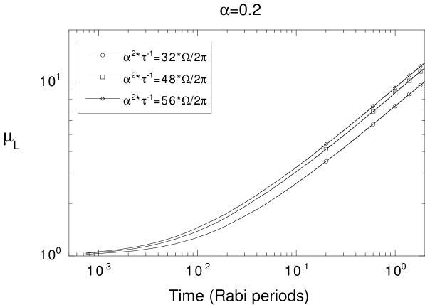
Figure 6: Temporal evolution of the mean $\mu_{L}$ introduced in Eq. (53), for $\alpha_{R}=\alpha_{L}=\alpha=0.2$ and $x=32,\ 48,\ 56$.

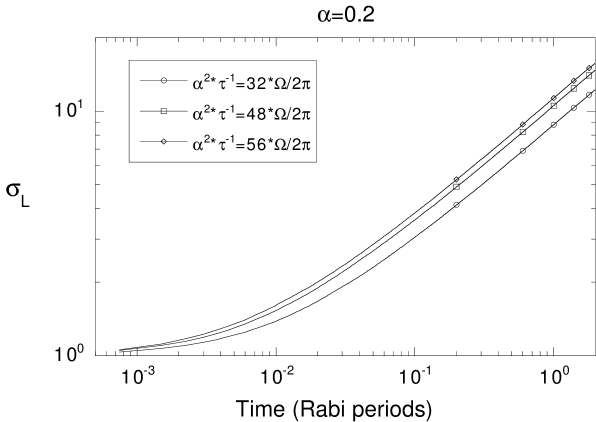
Figure 7: Temporal evolution of the standard deviation $\sigma_{L}$ introduced in Eq. (54), for $\alpha_{R}=\alpha_{L}=\alpha=0.2$ and $x=32,\ 48,\ 56$.

We now show how the relaxation of the population depends on the collision frequency $\tau^{-1}$, for fixed values of the parameter $\alpha=\alpha_{L}=\alpha_{R}$. 8 shows the temporal evolution of the relative population of the left subspace $P_{L}(t)\equiv\sum_{n_{L}}p_{n_{L}}(t)$ (once again, the analytical results cannot be distinguished from the numerical ones and are not shown in the graph). We note that this quantity will always eventually tend to its equilibrium value $P_{L}^{*}=1/2$, according to (73). However, the important point is that by increasing the collision frequency from $300\ T_{R}^{-1}$ to $800\ T_{R}^{-1}$, the system tends to remain in the left subspace for a longer time. This is evident in the plot and is a clear manifestation of a QZE. We also notice (although this is not clearly visible in 8, due to the scale chosen) that there is always a short-time quadratic region, characterized by a ”Zeno time” $\ddot{P}_{L}(0)=-\Omega$, in full agreement with Eq. (68). The features of this short-time region are independent of other parameters (such as $\alpha$ and $\tau$) ⁹, as can be seen in the figure. Finally, we emphasize that $x=\alpha^{2}T/\tau$ ranges between 12 and 32 and is therefore always $\gg 1$, so that the analysis of Sec. 6.1 applies.

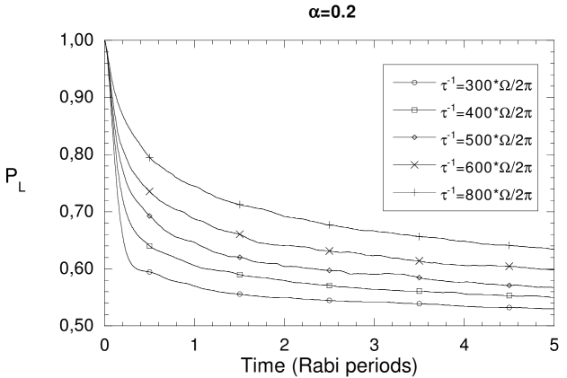
Figure 8: Temporal evolution of $P_{L}$ as a function of the collision frequency $\tau^{-1}$. We always set $\alpha=\alpha_{l}=\alpha_{R}=0.2$.

A similar Zeno effect is evident when the parameter $\alpha$ is varied, while keeping the collision frequency $\tau^{-1}$ constant, as displayed in 9 (once again, we only display the numerical results, for the analytical ones cannot be distinguished). Unlike in the preceding case, where the Zeno effect was due to increasing collision frequency, now it is due to increasing collision effectiveness: a larger $\alpha$ entails more dephasing and decoherence and, in a loose sense, a better ”measurement” of the quantum state. The parameter $x=\alpha^{2}T/\tau$ ranges between 39 and 72 ($\gg 1$) and one observes again the presence of a (parameter-independent) short-time region.

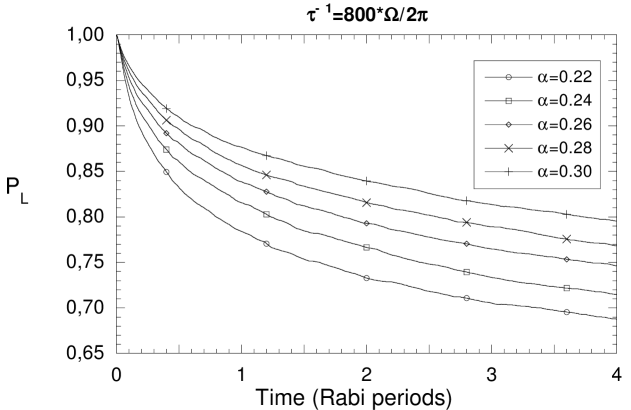
Figure 9: Temporal evolution of $P_{L}$ as a function of $\alpha=\alpha_{L}=\alpha_{R}$. For all calculations we set $\tau^{-1}=800\Omega/2\pi$.

As the analysis of Secs. 4-6 shows, the dynamics of the system should be ruled by the scaling parameter

$$x=DT_{R}=\frac{\alpha^{2}T_{R}}{\tau}.$$ (88)

10 shows how this scaling law is supported by the results of the numerical simulation. The plot shows three sets of curves corresponding to three different values of $x$. In each set, the values of $\alpha$ and $\tau$ were varied as indicated. Some deviations from the scaling law (of order 5%) can be observed and are to be ascribed to the influence of the terms neglected in deriving Eq. (36). Incidentally, notice again the short-time quadratic behavior.

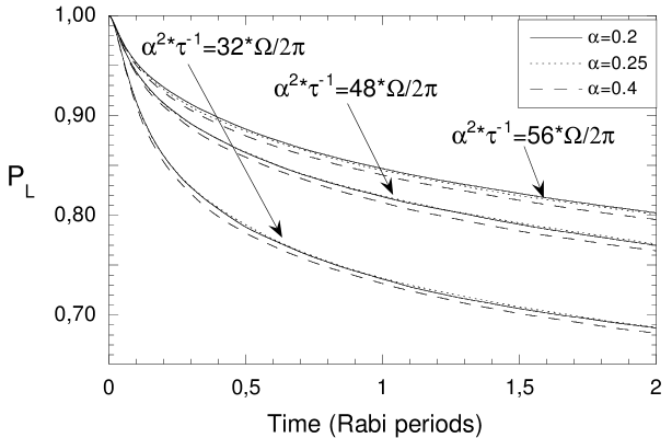
Figure 10: Test of the scaling law (88). Temporal evolution of $P_{L}$ for different values of $x=\alpha^{2}T/\tau$: three simulations were done with $\alpha_{R}=\alpha_{L}=\alpha=0.2,\ 0.25,\ 0.4$, respectively. $x$ ranges between 32 to 56.

8 Concluding remarks

We have studied a Zeno effect in a multilevel molecule made up of 40+40 levels, one of which (the ground state of the left subspace) is initially populated, and the evolution towards the right subspace is slowed down both because the collisions remove population density ”upwards” from the left ground state (a classically intuitive process) and because they ”dephase” (or analogously, make energetically less favorable) the transitions towards the right subspace. The latter process is classically less intuitive, but is readily understood if one thinks in terms of quantum transition amplitudes (or of the Fermi ”golden” rule for a bona fide unstable system).

It is worth stressing that the general ideas and techniques introduced in this article are valid for any multilevel molecule and any possible level distribution: we focused on the case (9) only for concreteness. Those situations in which (28) is not valid are very particular cases and their analysis, although of interest, goes beyond the scope of this article.

On the other hand, it is also necessary to emphasize that we neglected temperature effects and rapid structural rearrangement phenomena leading to a Boltzmann distribution of the level populations. This is a conceptually interesting problem, that involves delicate issues: a sensible estimate of the timescales involved in these thermalization processes is a challenging problem that requires further investigation.

We conclude by noticing that the Hamiltonian (1)-(6) is also relevant for the study of quantum chaos and Anderson localization ³⁵. The analysis of Poissonianly distributed ”kicks” (7) would introduce a novel element of discussion in such a context.

P.F. and S.P. acknowledge the financial support of the European Union through the Integrated Project EuroSQIP. D.B., S.L. and P.M. were partially supported by Ministero dell’Istruzione, dell’Università e della Ricerca (Contract 2001031223_009).

9 Appendix

It is interesting to look explicitly at the derivation of Eq. (36) from Eq. (27). The physical mechanism at work is the effective decoupling between the fast and the slow modes in (27). Let us start from the equation for $\rho_{1_{L}2_{L}}$, that explicitly reads [here $\omega_{2_{L}1_{L}}\equiv\left(E_{2_{L}}-E_{1_{L}}\right)/\hbar$]

$$\frac{d\rho_{1_{L}2_{L}}}{dt} = i\omega_{2_{L}1_{L}}\rho_{1_{L}2_{L}}-i\Omega\rho_{1_{R}2_{L}}-i\frac{\alpha_{L}}{\tau}\left(\rho_{2_{L}2_{L}}-\rho_{1_{L}1_{L}}-\rho_{1_{L}3_{L}}\right)$$ (89)

$$-\frac{\alpha^{2}_{L}}{2\tau}(\rho_{1_{L}2_{L}}+\rho_{3_{L}2_{L}}-2\rho_{2_{L}1_{L}}-2\rho_{2_{L}3_{L}}+2\rho_{1_{L}2_{L}}+\rho_{1_{L}4_{L}}).$$

When condition (28) is satisfied, the first term in the right-hand side dominates over the others and one obtains

$$\frac{d\rho_{1_{L}2_{L}}}{dt}\simeq i\omega_{2_{L}1_{L}}\rho_{1_{L}2_{L}},$$ (90)

which yields a very fast dynamics for the term $\rho_{1_{L}2_{L}}$:

$$\rho_{1_{L}2_{L}}(t)=\rho_{1_{L}2_{L}}(0)\exp({i\omega_{2_{L}1_{L}}t}).$$ (91)

The equations for the other off-diagonal components of $\rho$ are similar. These equations yield very rapidly oscillating solutions.

On the other hand, the dynamics of the populations $\rho_{1_{s}1_{s}}$, with $s=L,R$, and of the coherent terms $\rho_{1_{L}1_{R}}$ is governed by the equations

$$\frac{d\rho_{1_{L}1_{L}}}{dt} = -i\Omega(\rho_{1_{R}1_{L}}-\rho_{1_{L}1_{R}})+\frac{\alpha_{L}^{2}}{\tau}(\rho_{2_{L}2_{L}}-\rho_{1_{L}1_{L}})-i\frac{\alpha_{L}}{\tau}(\rho_{2_{L}1_{L}}-\rho_{1_{L}2_{L}})-\frac{\alpha^{2}_{L}}{2\tau}(\rho_{3_{L}1_{L}}+\rho_{1_{L}3_{L}}),$$

$$\frac{d\rho_{1_{R}1_{R}}}{dt} = i\Omega(\rho_{1_{R}1_{L}}-\rho_{1_{L}1_{R}})+\frac{\alpha_{R}^{2}}{\tau}(\rho_{2_{R}2_{R}}-\rho_{1_{R}1_{R}})-i\frac{\alpha_{R}}{\tau}(\rho_{2_{R}1_{R}}-\rho_{1_{R}2_{R}})-\frac{\alpha^{2}_{R}}{2\tau}(\rho_{3_{R}1_{R}}+\rho_{1_{R}3_{R}}),$$

$$\frac{d\rho_{1_{L}1_{R}}}{dt} = i\Omega(\rho_{1_{L}1_{L}}-\rho_{1_{R}1_{R}})-\frac{\alpha_{L}^{2}}{2\tau}\rho_{1_{L}1_{R}}-\frac{\alpha_{R}^{2}}{2\tau}\rho_{1_{R}1_{L}}-i\frac{\alpha_{L}}{\tau}\rho_{2_{L}1_{R}}-i\frac{\alpha_{R}}{\tau}\rho_{1_{L}2_{R}}+\frac{\alpha_{L}\alpha_{R}}{\tau}\rho_{2_{L}2_{R}}$$ (92)

$$-\frac{\alpha^{2}_{L}}{2\tau}\rho_{3_{L}1_{R}}-\frac{\alpha^{2}_{R}}{2\tau}\rho_{1_{L}3_{R}}.$$

It is apparent that no ”diagonal” fast frequency $\omega$ is present and these matrix elements evolve over timescales $\tau$ and $\Omega^{-1}$ which are much larger than $\omega^{-1}$. Therefore the contribution of all the off-diagonal fast terms of the type (91) is averaged to zero over the long timescales $\tau$ and $\Omega^{-1}$, the dynamics of the slow and fast terms completely decouples and we get

$$\frac{d\rho_{1_{L}1_{L}}}{dt} \simeq -i\Omega(\rho_{1_{R}1_{L}}-\rho_{1_{L}1_{R}})+\frac{\alpha_{L}^{2}}{\tau}(\rho_{2_{L}2_{L}}-\rho_{1_{L}1_{L}}),$$

$$\frac{d\rho_{1_{R}1_{R}}}{dt} \simeq i\Omega(\rho_{1_{R}1_{L}}-\rho_{1_{L}1_{R}})+\frac{\alpha_{R}^{2}}{\tau}(\rho_{2_{R}2_{R}}-\rho_{1_{R}1_{R}}),$$

$$\frac{d\rho_{1_{L}1_{R}}}{dt} \simeq i\Omega(\rho_{1_{L}1_{L}}-\rho_{1_{R}1_{R}})-\frac{\alpha_{L}^{2}}{2\tau}\rho_{1_{L}1_{R}}-\frac{\alpha_{R}^{2}}{2\tau}\rho_{1_{R}1_{L}}.$$

Analogously, the evolution equations of the populations $p_{m_{s}}=\rho_{m_{s}m_{s}}$ read ($m_{s}\neq 1_{L,R}$)

$$\frac{d\rho_{m_{s}m_{s}}}{dt} = \frac{\alpha^{2}_{s}}{\tau}\left(\rho_{m_{s}-1,m_{s}-1}-2\rho_{m_{s}m_{s}}+\rho_{m_{s}+1,m_{s}+1}\right)$$ (94)

$$-i\frac{\alpha_{s}}{\tau}\left(\rho_{m_{s}+1,m_{s}}-\rho_{m_{s},m_{s}+1}+\rho_{m_{s}-1,m_{s}}-\rho_{m_{s},m_{s}-1}\right)$$

$$-\frac{\alpha^{2}_{s}}{2\tau}\left(\rho_{m_{s}-2,m_{s}}+\rho_{m_{s},m_{s}-2}+\rho_{m_{s}+2,m_{s}}+\rho_{m_{s},m_{s}+2}\right),$$

and by the same argument reduce to

$$\frac{d\rho_{m_{s}m_{s}}}{dt}\simeq\frac{\alpha^{2}_{s}}{\tau}\left(\rho_{m_{s}-1,m_{s}-1}-2\rho_{m_{s}m_{s}}+\rho_{m_{s}+1,m_{s}+1}\right),$$

which are in the form (29)-(36). Notice the absence of fast and oscillating terms.

References

- 1 B. Misra and E.C.G. Sudarshan, J. Math. Phys. 18, 756 (1977).
- 2 A. Beskow and J. Nilsson, Arkiv für Fysik 34, 561 (1967); L. A. Khalfin, JETP Letters 8, 65 (1968); C. N. Friedman, Indiana Univ. Math. J. 21, 1001 (1972); K. Gustafson, ”Irreversibility questions in chemistry, quantum-counting, and time-delay,” in Energy storage and redistribution in molecules, edited by J. Hinze (Plenum, 1983), and references [10,12] therein; K. Gustafson and B. Misra, Lett. Math. Phys. 1, 275 (1976).
- 3 J. von Neumann, Mathematical Foundation of Quantum Mechanics (Princeton University Press, Princeton, 1955). The QZE is discussed at p. 366.
- 4 R. J. Cook, Phys. Scr. T 21, 49 (1988); W. H. Itano, D. J. Heinzen, J. J. Bollinger, and D. J. Wineland, Phys. Rev. A 41, 2295 (1990); T. Petrosky, S. Tasaki, and I. Prigogine, Phys. Lett. A 151, 109 (1990); Physica A 170, 306 (1991); A. Peres and A. Ron, Phys. Rev. A 42, 5720 (1990); S. Pascazio, M. Namiki, G. Badurek, and H. Rauch, Phys. Lett. A 179, 155 (1993); T. P. Altenmüller and A. Schenzle, Phys. Rev. A 49, 2016 (1994); S. Pascazio and M. Namiki, Phys. Rev. A 50, 4582 (1994); P. Kwiat, H. Weinfurter, T. Herzog, A. Zeilinger, and M. Kasevich, Phys. Rev. Lett. 74, 4763 (1995); A. Venugopalan and R. Ghosh, Phys. Lett. A 204, 11 (1995); A. Beige and G. Hegerfeldt, Phys. Rev. A 53, 53 (1996).
- 5 J. I. Cirac, A. Schenzle, and P. Zoller, Europhys. Lett 27, 123 (1994); M. V. Berry and S. Klein, J. Mod. Opt. 43, 165 (1996); A. Luis and J. Periňa, Phys. Rev. Lett. 76, 4340 (1996); M. P. Plenio, P. L. Knight, and R. C. Thompson, Opt. Comm. 123, 278 (1996); E. Mihokova, S. Pascazio, and L. S. Schulman, Phys. Rev. A 56, 25 (1997); J. Řeháček et al, Phys. Rev. A 62, 013804 (2000); B. Militello, A. Messina, and A. Napoli Phys. Lett. A 286, 369 (2001); Fortschr. Phys. 49, 1041 (2001); G. S. Agarwal, M. O. Scully, and H. Walther, Phys. Rev. Lett. 86, 4271 (2001); E. Frishman and M. Shapiro, Phys. Rev. Lett. 87, 253001 (2001); A. D. Panov, Phys. Lett. A 298, 295 (2002).
- 6 A. M. Lane, Phys. Lett. A 99, 359 (1983); W. C. Schieve, L. P. Horwitz, and J. Levitan, Phys. Lett. A 136, 264 (1989); S. A. Gurvitz, Phys. Rev. B 56, 15215 (1997); P. Facchi and S. Pascazio Phys. Rev. A 62, 023804 (2000); A. G. Kofman and G. Kurizki, Nature 405, 546 (2000); P. Facchi, H. Nakazato, and S. Pascazio, Phys. Rev. Lett. 86, 2699 (2001); M.C. Fischer, B. Gutiérrez-Medina, and M.G. Raizen, Phys. Rev. Lett. 87, 040402 (2001).
- 7 A. Peres, Am. J. Phys. 48, 931 (1980); K. Kraus, Found. Phys. 11, 547 (1981); A. Sudbery, Ann. Phys. 157, 512 (1984); L.S. Schulman, Phys. Rev. A 57, 1509 (1998); P. Facchi and S. Pascazio, ”Quantum Zeno effects with ”pulsed” and ”continuous” measurements”, in Time’s arrows, quantum measurements and superluminal behavior, edited by D. Mugnai, A. Ranfagni, and L. S. Schulman (CNR, Rome, 2001) p. 139; Fortschritte der Physik 49, 941 (2001).
- 8 H. D. Zeh, Found. Phys. 1, 69 (1970); M. Simonius, Phys. Rev. Lett. 40, 980 (1978); R. A. Harris and L. Stodolsky, J. Chem. Phys. 74, 2145 (1981); Phys. Lett. B 116, 464 (1982).
- 9 P. Facchi and S. Pascazio, ”Quantum Zeno and inverse quantum Zeno effects,” in: Progress in Optics 42, edited by E. Wolf, Elsevier Amsterdam, 2001, p. 147.
- 10 For a review, see H. Nakazato, M. Namiki and S. Pascazio, Int. J. Mod. Phys. B 10, 247 (1996); D. Home and M.A.B. Whitaker, Ann. Phys. 258, 237 (1997). For experimental confirmation, see S. R. Wilkinson, C. F. Bharucha, M. C. Fischer, K. W. Madison, P. R. Morrow, Q. Niu, B. Sundaram, and M. G. Raizen, Nature 387, 575 (1997).
- 11 P. Facchi, V. Gorini, G. Marmo, S. Pascazio, and E. C. G. Sudarshan, Phys. Lett. A 275, 12 (2000); P. Facchi, S. Pascazio, A. Scardicchio, and L. S. Schulman, Phys. Rev. A 65, 012108 (2002). See also K. Machida, H. Nakazato, S. Pascazio, H. Rauch, and S. Yu, Phys. Rev. A 60, 3448 (1999).
- 12 P. Facchi and S. Pascazio, Phys. Rev. Lett. 89, 080401 (2002).
- 13 P. Facchi and S. Pascazio, J. Phys. A: Math. Theor. 41 493001 (2008).
- 14 Kwiat R, Weinfurter H, Herzog T, Zeilinger A, and Kasevich M 1995 Phys. Rev. Lett. 74 4763
- 15 B. Nagels, L.J.F. Hermans and P.L. Chapovsky, Phys. Rev. Lett. 79, 3097 (1997).
- 16 Balzer C, Huesmann R, Neuhauser W and Toschek P E 2000 Opt. Comm. 180 115
- 17 Toschek P E and Wunderlich C 2001 Eur. Phys. J. D 14 387
- 18 Wunderlich C, Balzer C and Toschek P E 2001 Z. Naturforsch. 56a 160
- 19 Balzer C, Hannemann T, Reib D, Wunderlich C, Neuhauser W and Toschek P E 2002 Opt. Commun. 211 235
- 20 Mølhave K and Drewsen M 2000 Phys. Lett. A 268 45
- 21 Xiao L and Jones J A 2006 Physics Letters A 359 424
- 22 Streed E W, Mun J, Boyd M, Campbell G K, Medley P, Ketterle W and Pritchard D E 2006 Phys. Rev. Lett. 97 260402
- 23 J. Bernu, S. Deléglise, C. Sayrin, S. Kuhr, I. Dotsenko, M. Brune, J.-M. Raimond and S. Haroche, Phys. Rev. Lett. 101, 180402 (2008)
- 24 Jericha E, Schwab D E, Jäkel M R, Carlile C J and Rauch H 2000 Physica B 283 414
- 25 Rauch H 2001 Physica B 297 299
- 26 P.L. Chapovsky, Phys. Rev. A 43, 3624 (1991); Physica A 233, 441 (1996); B. Nagels, M. Schuurman, P.L. Chapovsky and L.J.F. Hermans, Phys. Rev. A 54, 2050 (1996).
- 27 P.L. Chapovsky and L.J.F. Hermans, Ann. Rev. Phys. Chem. 50, 315 (1999).
- 28 E. W. Montroll, K. E. Shuler, Advan. Chem. Phys. 1, 361 (1958); M. Capitelli and E. Molinari, Kinetics of Dissociation Processes in Plasmas in the low and Intermediate Pressure Range, Topics in Current Chemistry, vol. 90, Springer (1980).
- 29 S. Longo, D. Bruno, M. Capitelli, P. Minelli, Chem. Phys. Lett 316, 311 (2000); S. Longo, D. Bruno, P. Minelli, Chem. Phys. 256, 265 (2000).
- 30 S. Longo, Phys. Lett. A 267, 117 (2000); S. Longo, D. Bruno, Chem. Phys. 264, 211 (2001).
- 31 C. W. Gardiner, Handbook of Stochastic Methods (Springer, Berlin 1983).
- 32 V. Gorini, A. Frigerio, M. Verri, A. Kossakowski, and E. C. G. Sudarshan, J. Math. Phys. (N.Y.) 17, 821 (1976); G. Lindblad, Commun. Math. Phys. 48, 119 (1976); R. Alicki and K. Lendi, Quantum Dynamical Semigroups and Applications, Lecture Notes in Physics Vol. 286 (Springer-Verlag, Berlin, 1987).
- 33 N. G. Van Kampen, Stochastic processes in physics and chemistry (Elsevier, Amsterdam 1992).
- 34 I. S. Gradshteyn and I. M. Ryzhik, Table of Integrals, Series, and Products (Academic Press, San Diego, 1994).
- 35 B. Kaulakys and V. Gontis, Phys. Rev. A 56, 1131 (1997); P. Facchi, S. Pascazio and A. Scardicchio, Phys. Rev. Lett. 83, 61 (1999); J.C. Flores, Phys. Rev. B 60, 30 (1999); B 62, R16291 (2000); A. Gurvitz, Phys. Rev. Lett. 85, 812 (2000); J. Gong and P. Brumer, Phys. Rev. Lett. 86, 1741 (2001); M.V. Berry, ”Chaos and the semiclassical limit of quantum mechanics (is the moon there when somebody looks?),” in Quantum Mechanics: Scientific perspectives on divine action (eds: Robert John Russell, Philip Clayton, Kirk Wegter-McNelly and John Polkinghorne), Vatican Observatory CTNS publications, p. 41.