Statistical Properties of Eigenvalues for an Operating Quantum Computer with Static Imperfections

Abstract

We investigate the transition to quantum chaos, induced by static imperfections, for an operating quantum computer that simulates efficiently a dynamical quantum system, the sawtooth map. For the different dynamical regimes of the map, we discuss the quantum chaos border induced by static imperfections by analyzing the statistical properties of the quantum computer eigenvalues. For small imperfection strengths the level spacing statistics is close to the case of quasi-integrable systems while above the border it is described by the random matrix theory. We have found that the border drops exponentially with the number of qubits, both in the ergodic and quasi-integrable dynamical regimes of the map characterized by a complex phase space structure. On the contrary, the regime with integrable map dynamics remains more stable against static imperfections since in this case the border drops only algebraically with the number of qubits.

1 Introduction

Quantum computers, if constructed, would be capable of solving some computational problems much more efficiently than classical computers chuang . Shor shor constructed a quantum algorithm which performs integer factorization exponentially faster than any known classical algorithm. It was also shown by Grover grover that the search of an item in an unstructured list can be done with a square root speedup over any classical algorithm. These results motivated a great body of experimental proposals for the construction of a realistic quantum computer (see chuang and references therein).

While the technological challenge to develop scalable, fault tolerant quantum processors is highly demanding, it is well appreciated that decoherence, due to the coupling with the environment, will be the ultimate obstacle to the realization of such devices. In addition, even in the ideal case in which the quantum computer is isolated from the external world, a proper operability of the computer is not guaranteed: unavoidable internal static imperfections in the quantum computer hardware represent another source of errors. For example, the energy spacing between the two states of each qubit can fluctuate, e.g. due to magnetic field inhomogeneities in nuclear magnetic resonance quantum processors chuang . Moreover, since qubit interactions are required to operate two-qubit gates and generate entangled states, unwanted residual interactions will appear. For example, when the inter-qubit coupling is switched off, e.g. via a potential barrier created by a point contact gate in the quantum dots proposal loss , some unavoidable residual interactions still remain. Therefore the quantum computer hardware can be modeled as a qubit lattice and one has to consider it as a quantum many-qubit (-body) interacting system GS . Many-body quantum systems have been widely investigated in the field of quantum chaos bohigas ; guhr and it is now well known that residual interactions can lead to quantum chaos characterized by ergodicity of the eigenstates and level spacing statistics described by random matrix theory aberg ; jacquod ; JLP ; flambaum . In the regime of quantum chaos the wave functions and energy spectra become so complicated that a statistical description should be applied to them. Thus it is important to study the stability of quantum information processing in the presence of realistic models of quantum computer hardware imperfections and in concrete examples of quantum algorithms. The stability of the static quantum computer hardware was studied in GS and it was shown that residual inter-qubit interactions can destroy a generic state stored in the quantum computer if the amplitude of static imperfections is above the quantum chaos border. For a static quantum hardware this border drops linearly with the number of qubits while the average energy level spacing drops exponentially. Above the quantum chaos border an exponential number of ideal multi-qubit states becomes mixed after a finite chaotic time scale. The implications of such imperfections for the Grover algorithm and quantum Fourier transform were analyzed in Ref. braun .

In this paper, we address the question of the transition to chaos for an operating quantum computer, which is running an efficient quantum algorithm simulating the dynamical evolution of the so-called quantum sawtooth map simone1 . The sawtooth map is a paradigm of classical sawc and quantum sawq chaos, and exhibits a variety of different behaviors, from anomalous diffusion to quantum ergodicity and dynamical localization. We note that in the above quantum algorithm the number of redundant qubits can be reduced to zero and complex dynamics can be investigated already with less than 10 qubits. It is therefore important to study the stability of such algorithm, in view of its possible implementation in the first generation of quantum processors operating with a small number of qubits qftexp ; shorexp .

Since spectral statistics is the most valuable tool to detect the transition to quantum chaos bohigas ; guhr , we study the statistical properties of the eigenvalues of the quantum sawtooth map, simulating different dynamical regimes (ergodic, quasi-integrable, and integrable), in the presence of static imperfections in the quantum computer hardware. We will show that the threshold for the transition to chaos induced by static imperfections drops exponentially with the number of qubits both in the ergodic and in the quasi-integrable regime, while in the integrable regime the chaos border drops only polynomially with the number of qubits. We note that this paper complements Ref. simone2 , devoted to the study of the eigenvectors of the model in the ergodic regime.

The paper is organized as follows. In Section 2 we discuss the quantum algorithm simulating the quantum sawtooth map model and its realization in the presence of hardware static imperfections. The effect of these imperfections on the spectral statistics of the model is described in Sections 3,4, and 5, for the ergodic, quasi-integrable, and integrable regime, respectively. Our conclusions are presented in Section 6.

2 The model and the quantum algorithm

The quantum sawtooth map is the quantized version of the classical sawtooth map, which is given by

$$\overline{n}={n}+k(\theta-\pi),\quad\overline{\theta}=\theta+T\overline{n},$$ (1)

where $(n,\theta)$ are conjugated action-angle variables ($0\leq\theta<2\pi$), and the bars denote the variables after one map iteration. Introducing the rescaled momentum variable $p=Tn$, one can see that the classical dynamics depends only on the single parameter $K=kT$. As it is known, the classical motion is stable for $-4<K<0$ and completely chaotic for $K<-4$ and $K>0$ sawc .

The quantum evolution for one map iteration is described by a unitary operator $\hat{U}_{0}$ (Floquet operator) acting on the wave function $\psi$:

$$\overline{\psi}=\hat{U}_{0}\psi=e^{-iT\hat{n}^{2}/2}e^{ik(\hat{\theta}-\pi)^{2}/2}\psi,$$ (2)

where $\hat{n}=-i\partial/\partial\theta$ and $\psi(\theta+2\pi)=\psi(\theta)$ (we set $\hbar=1$). The classical limit corresponds to $k\to\infty$, $T\to 0$, and $K=kT=\hbox{const}$.

In this paper, we study the quantum sawtooth map (2) closed on the torus $-\pi\leq p<\pi$. Therefore the classical limit is obtained by increasing the number of qubits $n_{q}=\log_{2}N$ ($N$ is the total number of levels), with $T=2\pi/N$ ($k=K/T$, $-N/2\leq n<N/2$). We consider the ergodic, quasi-integrable and integrable regimes. To this end, we take $K=\sqrt{2}$, $K=-0.1$, and $K=-1$, respectively.

The quantum algorithm introduced in simone1 simulates efficiently the quantum dynamics (2) using a register of $n_{q}$ qubits. It is based on the forward/backward quantum Fourier transform qft between the $\theta$ and $n$ representations and has some elements of the quantum algorithm for kicked rotator GS1 . Such an approach is rather convenient since the Floquet operator $\hat{U}_{0}$ is the product of two operators $\hat{U}_{k}=e^{ik(\hat{\theta}-\pi)^{2}/2}$ and $\hat{U}_{T}=e^{-iT\hat{n}^{2}/2}$: the first one is diagonal in the $\hat{\theta}$ representation, the latter in the $\hat{n}$ representation. Thus the quantum algorithm for one map iteration requires the following steps:
I. The unitary operator $\hat{U}_{k}$ is decomposed in $n_{q}^{2}$ two-qubit gates

$$e^{\imath k(\theta-\pi)^{2}/2}=\prod_{i,j}e^{\imath 2\pi^{2}k(\alpha_{i}2^{-i}-\frac{1}{2n_{q}})(\alpha_{j}2^{-j}-\frac{1}{2n_{q}})},$$ (3)

where $\theta=2\pi\sum\alpha_{i}2^{-i}$, with $\alpha_{i}\in\{0,1\}$. Each two-qubit gate can be written in the $\{|00\rangle,|01\rangle,|10\rangle,|11\rangle\}$ basis as $\exp(ik\pi^{2}D)$, where D is a diagonal matrix with elements

$$\{\frac{1}{2n_{q}^{2}},-\frac{1}{n_{q}}\left(\frac{1}{2^{j}}-\frac{1}{2n_{q}}\right),-\frac{1}{n_{q}}\left(\frac{1}{2^{i}}-\frac{1}{2n_{q}}\right),$$

$$2\left(\frac{1}{2^{i}}-\frac{1}{2n_{q}}\right)\left(\frac{1}{2^{j}}-\frac{1}{2n_{q}}\right)\}.$$ (4)

II. The change from the $\theta$ to the $n$ representation is obtained by means of the quantum Fourier transform, which requires $n_{q}$ Hadamard gates and $n_{q}(n_{q}-1)/2$ controlled-phase shift gates qft .
III. In the new representation the operator $\hat{U}_{T}$ has essentially the same form as $\hat{U}_{k}$ in step I and therefore it can be decomposed in $n_{q}^{2}$ gates similarly to equation (3).
IV. We go back to the initial $\theta$ representation via inverse quantum Fourier transform.
On the whole the algorithm requires $3n_{q}^{2}+n_{q}$ gates per map iteration. Therefore it is exponentially efficient with respect to any known classical algorithm. Indeed the most efficient way to simulate the quantum dynamics (2) on a classical computer is based on forward/backward fast Fourier transform and requires $O(n_{q}2^{n_{q}})$ operations. We stress that this quantum algorithm does not need any extra work space qubit. This is due to the fact that for the quantum sawtooth map the kick operator $\hat{U}_{k}$ has the same quadratic form as the free rotation operator $\hat{U}_{T}$.

We model the quantum computer hardware as an linear array of qubits (spin halves) with static imperfections, i.e. fluctuations in the individual qubit energies and residual short-range inter-qubit couplings GS . The model is described by the following many-body Hamiltonian:

$$\hat{H}_{\hbox{s}}=\sum_{i}(\Delta_{0}+\delta_{i})\hat{\sigma}_{i}^{z}+\sum_{i<j}J_{ij}\hat{\sigma}_{i}^{x}\hat{\sigma}_{j}^{x},$$ (5)

where the $\hat{\sigma}_{i}$ are the Pauli matrices for the qubit $i$, and $\Delta_{0}$ is the average level spacing for one qubit. The second sum in (5) runs over nearest-neighbor qubit pairs, zero boundary conditions are applied, and $\delta_{i}$, $J_{ij}$ are randomly and uniformly distributed in the intervals $[-\delta/2,\delta/2]$ and $[-J,J]$, respectively. We model the implementation of the above described algorithm as a sequence of instantaneous and perfect one- and two-qubit gates, separated by a time interval $\tau_{g}$, during which the hardware Hamiltonian (5) gives unwanted phase rotations and qubit couplings. Therefore we study numerically the many-body Hamiltonian

$$\hat{H}(\tau)=\hat{H}_{\hbox{s}}+\hat{H}_{\hbox{g}}(\tau),$$ (6)

where

$$\hat{H}_{\hbox{g}}(\tau)=\sum_{k}\delta(\tau-k\tau_{g})\hat{h}_{k}.$$ (7)

Here $\hat{h}_{k}$ realizes the $k$-th elementary gate according to the sequence prescribed by the above algorithm. We assume that the average phase accumulation given by $\Delta_{0}$ is eliminated, e.g. by means of refocusing techniques chuang2 .

Since the evolution operator (2) remains periodic in the presence of static imperfections, $\hat{U}_{\epsilon,\rho}(\tau+T)=\hat{U}_{\epsilon,\rho}(\tau)$ ($\epsilon\equiv\delta\tau_{g}$, $\rho\equiv J\tau_{g}$ rescaled imperfection strengths), all information about the system dynamics is included in the quasi-energy eigenvalues $\lambda_{\alpha}^{(\epsilon,\rho)}$ and eigenstates $\phi_{\alpha}^{(\epsilon,\rho)}$ of the perturbed Floquet operator:

$$\hat{U}_{\epsilon,\rho}(T)\phi_{\alpha}^{(\epsilon,\rho)}=\exp(i\lambda_{\alpha}^{(\epsilon,\rho)})\phi_{\alpha}^{(\epsilon,\rho)}.$$ (8)

We study numerically the spectral statistics of the Floquet operator (8) for a quantum computer running the quantum sawtooth map algorithm in the presence of static imperfections described by (5). We construct numerically the Floquet operator in the momentum representation (i.e. the quantum register states basis) using the fact that the one step map evolution (including static imperfections) of each quantum register state gives a column in the matrix representation of this operator.

We consider $4\leq n_{q}\leq 12$ qubits. In order to reduce statistical fluctuations, data are averaged over $3\leq N_{D}\leq 10^{3}$ random realizations of static imperfections. In this way the total number of Floquet quasi-energies is $N_{D}\times 2^{n_{q}}\approx 10^{4}$, which is large enough to get stable results in the study of spectral statistics.

3 The ergodic regime

We focus our attention first on the ergodic regime, where the eigenfunctions of the unperturbed Floquet operator are given by a complex superposition of order $N=2^{n_{q}}$ quantum register states. In particular, we consider $K=\sqrt{2}$, where the corresponding classical sawtooth map (1) is completely chaotic. In the ideal case in the absence of static imperfections ($\epsilon=0$, $\rho=0$), the eigenvalues of the Floquet operator are divided in two different symmetry classes, even and odd with respect to the transformation $n\rightarrow-n$. Thus the Floquet operator has two blocks which can be studied independently. A convenient tool to characterize the spectral properties of the system is the level spacing statistics $P(s)$, giving the probability to find two consecutive eigenvalues whose energy difference, normalized to the average level spacing, is in $[s,s+ds]$. Since we are in the ergodic regime, the level spacing statistics for each block is well described by the random matrix theory bohigas ; guhr in the presence of time-reversal symmetry:

$$P_{O}(s)=\frac{\pi}{2}se^{-\pi s^{2}/4}.$$ (9)

This theoretical distribution is in agreement with the numerical results shown in the inset of Fig. 1 for the symmetric class. The global spectral statistics can be computed from the single spectral statistics of each symmetry class bohigas , and is given by:

$$P_{O}^{(2)}(s)=\frac{1}{2}\left(\hbox{erfc}\left(\frac{\sqrt{\pi}s}{4}\right)\frac{\pi s}{4}e^{-\pi s^{2}/16}+e^{-\pi s^{2}/8}\right),$$ (10)

again in good agreement with the numerical data of Fig. 1.

Figure 1: The level spacing distribution for $K=\sqrt{2}$, $n_{q}=11$ and $J=0$, at $\epsilon=0$ (circles) and $\epsilon=10^{-3}$ (squares). The dashed and full lines give the theoretical distribution (10) and (11), respectively. Inset: statistics for one symmetry class at $\epsilon=0$ and same parameter values as in the main figure. The dashed line is the theoretical distribution (9).

Since static imperfections break the time reversal symmetry, the two symmetry classes become mixed and the system undergoes a crossover from (10) to a different random matrix statistics bohigas ; guhr :

$$P_{U}(s)=\frac{32s^{2}}{\pi^{2}}e^{-4s^{2}/\pi}.$$ (11)

The good agreement between this limiting distribution and the actual statistics computed from numerical data is shown in Fig. 1 for $n_{q}=11$ and $\epsilon=10^{-3},J=0$. A convenient quantity to characterize the crossover from one limiting distribution to another is jacquod

$$\eta=\frac{\int_{0}^{s_{0}}(P(s)-P_{U}(s))ds}{\int_{0}^{s_{0}}(P_{O}^{(2)}(s)-P_{U}(s))ds}.$$ (12)

where $s_{0}=0.50285...$ is the first intersection point of $P_{O}^{(2)}(s)$ and $P_{U}(s)$. This parameter goes from one to zero, when the spacing probability changes from (10) to (11). The behavior of $\eta$ as a function of $\epsilon$ is shown in Fig. 2, for different $n_{q}$ values. This figure shows that it drops to zero when the imperfection strength grows. For $\epsilon\to 0$ and small $n_{q}$, there are significant deviations from the value $\eta=1$ corresponding to the limiting distribution (10). This is due to the fact that the $\epsilon=0$ statistics includes only $2^{n_{q}}$ levels spacings. For very small $\epsilon$ values the statistics remains poor since each static imperfections realization gives essentially the same $P(s)$ distribution. Nevertheless, it is clear that $\eta(\epsilon=0)$ goes to one when the number of qubits increases.

In order to study the dependence of the $\eta$-crossover on the number of qubits, we define the critical imperfections strength $\epsilon_{\chi}$ as the $\epsilon$ value at which $\eta=0.2$ (similar results are obtained for different $\eta$ values). In Fig. 3 we show that $\epsilon_{\chi}$ drops exponentially with the number of qubits. This exponential threshold is due to the fact that, in the ergodic regime, quantum eigenstates are given by a complex superposition of an exponentially large number of quantum register states. Indeed, due to quantum chaos, the eigenstates of the unperturbed ($\epsilon=0$, J=0) Floquet operator (8) can be written as

$$\phi_{\alpha}^{(0)}=\sum_{m=1}^{N}c_{\alpha}^{(m)}u_{m}.$$ (13)

Here $u_{m}$ are the quantum register states, and $c_{\alpha}^{(m)}$ are randomly fluctuating components, with $|c_{\alpha}^{(m)}|\sim 1/\sqrt{N}$ due to wave function normalization. The transition matrix elements between unperturbed eigenstates can be computed in perturbation theory. For $J=0$, they have a typical value

$$V_{\rm typ}\sim|\langle\phi_{\beta}^{(0)}|\sum_{i=1}^{n_{q}}\delta_{i}\hat{\sigma}_{i}^{z}\tau_{g}n_{g}|\phi_{\alpha}^{(0)}\rangle|$$

$$\sim\tau_{g}n_{q}^{2}|\sum_{m,n=1}^{N}c_{\alpha}^{(m)}c_{\beta}^{(n)\star}\sum_{i=1}^{n_{q}}\delta_{i}\langle u_{n}|\hat{\sigma}_{i}^{z}|u_{m}\rangle|$$ (14)

$$\sim\epsilon n_{q}^{5/2}|\sum_{m=1}^{N}c_{\alpha}^{(m)}c_{\beta}^{(m)\star}|\sim\epsilon n_{q}^{5/2}{N^{-1/2}}.$$

In this expression, the typical phase error is $\delta\sqrt{n_{q}}$ (sum of $n_{q}$ random detunings $\delta_{i}$’s) and $\tau_{g}n_{g}\sim\tau_{g}n_{q}^{2}$ is the time used by the quantum computer to simulate one map step. The last estimate in (14) results from the sum of $N$ terms of amplitude $|c_{\alpha}^{(m)}c_{\beta}^{(m)\star}|\sim 1/N$ and random phases. Since the spacing between quasi-energy eigenstates is $\Delta E\sim 1/N$, the threshold for the breaking of perturbation theory can be estimated as

$$V_{\rm typ}/\Delta E\sim\epsilon_{\chi}n_{q}^{5/2}\sqrt{N}\sim 1.$$ (15)

The analytical result

$$\epsilon_{\chi}\sim\frac{1}{n_{q}^{5/2}\sqrt{N}}$$ (16)

is confirmed by the numerical data of Fig. 3. For the case $J=\delta$, the threshold $\epsilon_{\chi}$ approximately decreases by a factor $1.2$ with respect to the $J=0$ case (see again Fig. 3), since residual inter-qubits interactions introduce further couplings between Floquet eigenstates. However, the same functional dependence (16) takes place.

Figure 2: Dependence of the $\eta$ parameter on the scale imperfection strength $\epsilon$ at $K=\sqrt{2}$, $J=0$. From right to left: $n_{q}=4,5,...,12$.

Figure 3: Dependence of the imperfections strength $\epsilon_{\chi}$ at which $\eta=0.2$ on the number of qubits, for $K=\sqrt{2}$, $J=0$ (diamonds) and $J=\delta$ (circles). The line gives the theoretical dependence $\epsilon_{\chi}=A2^{-n_{q}/2}n_{q}^{-2.5}$, with the fitting constant $A=4.3$.

We note that the same exponential sensitivity to static imperfections was detected for the Floquet eigenstates in Ref. simone2 . This confirms that spectral statistics are a useful tool to characterize the mixing of unperturbed eigenstates in an operating quantum computer.

4 The quasi-integrable regime

We now focus our study on the regime of quasi-integrability of the sawtooth map, in which the system is not chaotic (i.e. the Lyapunov exponent is zero) and there is a non integrable component in the phase space. In this situation, the system exhibits interesting physical properties, such as anomalous diffusion and hierarchical phase space structures simone1 . In this Section, we consider the case $K=-0.1$ and we study the transition to chaos for the eigenstates of a quantum computer simulating the quantum sawtooth map.

A useful tool to demonstrate the transition to chaos induced by static imperfections is the parametric dependence of the quasi-energy eigenvalues. The evolution of a part of the spectrum as a function of the imperfection strength $\epsilon$ (at $J=0$) is shown in Fig. 4. It makes evident the qualitative change induced by static imperfections. At small $\epsilon$ the spectrum exhibits quasi-degeneracyes, while at large $\epsilon$ avoided crossings appear. Indeed, at small $\epsilon$, Floquet eigenstates with very close eigenvalues may lay so far apart that their overlap is negligible. Thus there is essentially no level repulsion for these eigenvalues. On the contrary, at large $\epsilon$, Floquet eigenstates are delocalized and therefore their overlap is significant, and induces level repulsion haake . The delocalizing effect of static imperfections is evident in the Husimi functions of Fig. 5, drawn from two typical Floquet eigenstates husimi ; husimi1 .

Figure 4: Dependence of quasi-energy eigenvalues on the imperfections strength $\epsilon$, for $n_{q}=9$, $K=-0.1$, $J=0$. The thick dashed (dot-dashed) curves corresponds to the eigenvector represented in Fig. 5 right (left).

The two top plots of Fig. 5 represent two exact eigenstates ($\epsilon=0$, $J=0$). In the right picture, the quantum probability is concentrated around an ellipse corresponding to a classical integrable trajectory (a torus in the phase space $(\theta,p)$). We note that the map (1) is the discretized time evolution for an harmonic oscillator. Therefore it gives elliptic trajectories as far as border effects can be neglected. A completely different kind of eigenvector appears on the left picture. The Husimi function is spread, and this reflects the properties of the corresponding classical non-integrable trajectories which diffuse in a non-Brownian way simone1 . We note that the number of such eigenstates is non-negligible. Indeed, we have checked that the probability of finding a diffusive classical trajectory starting from a randomly chosen initial condition is 0.12. We also note that classical diffusion is suppressed by quantum interference effects giving a distribution localized in momentum. The remaining pictures of Fig. 5 represent the same Floquet eigenstates, computed in the presence of static imperfections. The middle figures are obtained slightly below the chaos border induced by static imperfections, and maintain same similarities with the exact eigenstates. On the contrary, in the bottom pictures, taken above the chaos border, the eigenfunctions are spread in all the available phase space and any structure has been destroyed. We note that, starting from completely different unperturbed eigenfunctions, one gets statistically indistinguishable eigenfunctions with randomly fluctuating components.

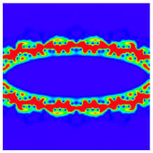
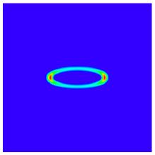
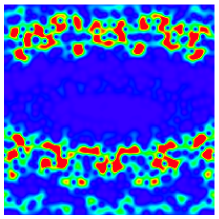
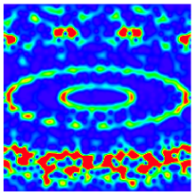
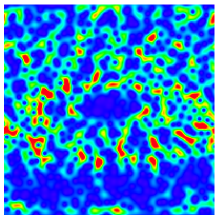
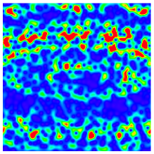
Figure 5: Husimi functions in action-angle variable $(p,\theta)$ ($-\pi\leq p<\pi$ -vertical axis- and $0\leq\theta<2\pi$ -horizontal axis-) for the quantum sawtooth map at $n_{q}=9$, $K=-0.1$, $J=0$. The left (right) column corresponds to the dot-dashed (dashed) line in Fig. 4, for $\epsilon=0$ (top), $\epsilon=10^{-3}$ (middle), $\epsilon=3\times 10^{-3}$ (bottom). We choose the ratio of the action-angle uncertainties $s=\Delta p/\Delta\theta=T\Delta n/\Delta\theta=1$ ($\Delta p\Delta\theta=T/2$). The color is proportional to the density: blue for zero and red for maximal density.

We now characterize the transition by studying the spectral statistics. In this regime, the limiting $P(s)$ distribution at $\epsilon=0$ is non trivial. Indeed, the Shnirelman theorem states that for a nearly integrable system the level spacing statistics $P(s)$ exhibits a huge peak near the origin ($s=0$) shni ; chirdima . In the following we choose to eliminate such peak, related to time-reversal invariance ($n\to-n$, $\theta\to 2\pi-\theta$). To do that we operate the transformation felice

$$\left\{\begin{array}[]{l}n\to n+\phi,\\ \cr\theta\to\theta+\theta_{0},\end{array}\right.$$ (20)

where $\phi$ plays the role of an Aharonov-Bohm flux note . The spectral statistics is still complex since in the classical limit the phase space has two components, integrable and non integrable. In the semi-classical limit, the levels belonging to these two components become uncorrelated and the global spacing statistics is given by the superposition of each component’s statistics berry . We note that in this case both components have non-trivial statistics. In particular it has been shown that for the related harmonic oscillator case the quasi-energy spectral statistics exhibits level repulsion and a finite number of peaks bohigas1 , instead of the Poisson statistics typical of integrable systems.

Figure 6: Level spacing distribution for $n_{q}=11$, $K=-0.1$, $\theta_{0}=\phi=\sqrt{2}/5$, $J=0$, $\epsilon=0$ (circles) and $\epsilon=10^{-3}$ (squares). The solid line gives the Wigner-Dyson distribution (Eq. (11)).

The spectral statistics at $\epsilon=0$, $J=0$ is shown in Fig. 6, for $n_{q}=11$. In the same figure, one can see that static imperfections induce a crossover to the Wigner-Dyson distribution (11). One can compare this figure with Fig. 1. The $\epsilon=0$ distributions are completely different, reflecting different dynamical regimes. On the contrary, the same universal distribution is found in the regime in which static imperfections destroy all symmetries. Even though in this case we cannot provide an analytical expression for the $\epsilon=J=0$ statistics, the crossover to the Wigner-Dyson distribution (11) can be characterized by the parameter

$$\tilde{\eta}=\left(\int_{0}^{+\infty}[P(s)-P_{U}(s)]^{2}ds\right)^{1/2},$$ (21)

measuring the distance of the spacing distribution from (11). The behavior of $\tilde{\eta}$ as a function of $\epsilon$ (at $J=0$) is shown in Fig. 7 for various $n_{q}$ values. This figure shows again that the Wigner -Dyson distribution ($\tilde{\eta}=0$) is reached by increasing $\epsilon$.

Figure 7: Dependence of the parameter $\tilde{\eta}$ on the imperfection strength $\epsilon$ for $K=-0.1$, $\theta_{0}=\phi=\sqrt{2}/5$, $J=0$. From right to left: $n_{q}=4,5,\dots,12$.

Similarly to what we have done in the ergodic regime, we define a critical imperfections strength $\epsilon_{\chi}$ as the $\epsilon$ value at which $\tilde{\eta}=0.2$. The dependence of $\epsilon_{\chi}$ on the number of qubits is shown in Fig. 8. Quite surprisingly, even in this quasi-integrable regime we can fit the exponential drop of $\epsilon_{\chi}$ with $n_{q}$ via the analytical function $\epsilon_{\chi}=B2^{-n_{q}/2}n_{q}^{-5/2}$, with the fitting constant $B=6.5$. Therefore, it seems that the theoretical argument developed in the previous Section for ergodic eigenstates has a broader validity and can apply also in the more general mixed phase space dynamics.

The same exponential sensitivity to static imperfections can be detected also in the Floquet eigenstates. The mixing of unperturbed eigenstates, induced by static imperfections, is characterized by the quantum eigenstates entropy

$$S_{\alpha}=-\sum_{\beta=1}^{N}p_{\alpha\beta}\log_{2}p_{\alpha\beta},$$ (22)

where $p_{\alpha\beta}=|\langle\phi_{\beta}^{(0)}|\phi_{\alpha}^{(\epsilon,\rho)}\rangle|^{2}$. In this way $S_{\alpha}=0$ if $\phi_{\alpha}^{(\epsilon,\rho)}$ coincides with one eigenstate at $\epsilon=\rho=0$, $S_{\alpha}=1$ if $\phi_{\alpha}^{(\epsilon,\rho)}$ is equally composed of two ideal ($\epsilon=\rho=0$) eigenstates, and $S_{\alpha}=n_{q}$ (maximal value) if all $\phi_{\beta}^{(0)}$ $(\beta=1,...,N=2^{n_{q}})$ contribute equally to $\phi_{\alpha}^{(\epsilon,\rho)}$. In Fig. 8 we show that the critical imperfection strength at which $S=1$ drops exponentially with the number of qubits ($S$ is the average of $S_{\alpha}$ over $\alpha$ and static imperfection realizations). This shows that the transition to chaos can be characterized both by the mixing of unperturbed eigenstates and by the transition in the spectral statistics.

Figure 8: Dependence of the imperfections strength $\epsilon_{\chi}$ at which $\tilde{\eta}=0.2$ (see Fig. 7) on the number of qubits $n_{q}$ (diamonds), for $K=-0.1$, $\theta_{0}=\phi=\sqrt{2}/5$, $J=0$. Squares give the critical imperfection strengths at which the quantum eigenstates entropy $S=1$. Lines give the theoretical dependency $\epsilon_{\chi}=BN^{-1/2}n_{q}^{-5/2}$, with the fitting constant $B=1$ (below) and $B=6.5$ (above).

5 The integrable regime

We now consider the integrable case $K=-1$. Independently of $n_{q}$, the quasi-energy spectrum is composed of 6 degenerate levels (see Fig.9), $\lambda^{(j)}=(2\pi/6)j$ (up to an unessential global phase factor). This phenomenon can be explained from classical mechanics: indeed the 6-th iterate of the map (1) gives the identity, i.e. all orbits are periodic with period at most 6 creutz . The same phenomenon can be observed at $K=-2$ ($K=-3$), where the spectrum has a degeneracy 4 (3) and the 4-th (third) iterate of (1) is the identity. In these cases, the quantum evolution and the classical discretized evolution coincide: this means that the quantum unitary evolution (2) maps a given phase space distribution in the same way as the discretized Liouville operator does in classical mechanics (see, e.g., Ref. saraceno ).

Figure 9: Quasi-energy levels $\lambda_{\alpha}$ at $n_{q}=9$, $K=-1$, $\epsilon=J=0$ (thick bands) and theoretical values (dashed lines).

Figure 10: Dependence of the imperfections strength $\epsilon_{\chi}$ at which $\tilde{\eta}=0.2$ on the number of qubits $n_{q}$, for $K=-1$, $J=0$ (diamonds) and $J=\delta$ (circles); note the log-log scale. Lines give the theoretical dependence $\epsilon_{\chi}=Cn_{q}^{-5/2}$, with the fitting constant $C=1$ (below) and $C=1.8$ (above).

Static imperfections induce a crossover to the universal Wigner-Dyson distribution (11), that can be characterized by the parameter $\tilde{\eta}$ defined in Eq. (21). Again, one can define a critical imperfection strength $\epsilon_{\chi}$ as the value of $\epsilon$ at which $\tilde{\eta}(\epsilon_{\chi})=0.2$. The result is shown in Fig. 10, where it is seen that $\epsilon_{\chi}$ drops polynomially with $n_{q}$: $\epsilon_{\chi}\propto n_{q}^{-5/2}$. This happens both for $J=0$ and $J=\delta$. We note that this algebraic dependence contrasts the exponential decay observed in previous Sections for the ergodic and quasi-integrable regimes. This can be understood via the following argument. Quantum ergodicity can be reached only when levels of the different bands of Fig. 9 are mixed. Non-degenerate levels are separated by an energy spacing $\Delta E$ which is $N$-independent. On the other hand, also the typical overlap between nearby eigenstates (in space) is $N$-independent (their space separation drops with $N$, but also their typical width drops with $N$). Since the typical error is $\delta\sqrt{n_{q}}$ and the time needed to simulate one map step is $\sim\tau_{g}n_{q}^{2}$ (see the discussion following Eq. (14)), one can estimate the typical transition matrix element $V_{\rm typ}\sim\epsilon n_{q}^{5/2}$, and the threshold for the breaking of perturbation theory as

$$V_{\rm typ}/\Delta E\sim\epsilon_{\chi}n_{q}^{5/2}\sim 1,$$ (23)

giving the analytical estimate

$$\epsilon_{\chi}\sim n_{q}^{-5/2}.$$ (24)

6 Conclusions

In this paper, we have studied the transition to quantum chaos, induced by static imperfections, in the spectral statistics of an operating quantum computer. The threshold for the transition to chaos drops exponentially with the number of qubits, both in the ergodic and in the more general quasi-integrable regime. On the contrary, in the integrable regime the chaos border drops only algebraically with the number of qubits. This is due to the presence of a finite number of bands in the spectrum of the time evolution operator related to global periodicity of classical dynamics. We note that similar strong spectral degeneracyes have been observed in the Grover’s algorithm and in the quantum Fourier transform in Ref. braun . We also stress that a complex dynamical system is generically quasi-integrable. The simulation of such systems is well accessible to the first generation of quantum computers with less than 10 qubits and we think that this class of quantum algorithms deserves further studies.

This work was supported in part by the EC RTN contract HPRN-CT-2000-0156 and by the NSA and ARDA under ARO contracts No. DAAD19-01-1-0553 (for D.L.S.) and No. DAAD19-02-1-0086. Support from the PRIN-2000 “Chaos and localization in classical and quantum mechanics” is gratefully acknowledged.

References

- (1) M.A. Nielsen and I.L. Chuang, Quantum Computation and Quantum Information (Cambridge University Press, Cambridge, 2000).
- (2) P. Shor, in Proceedings of the -th Annual Symposium on Foundations of Computer Science, edited by S. Goldwasser (IEEE Computer Society Press, Los Alamitos, CA, 1994), p. 124.
- (3) L.K. Grover, Phys. Rev. Lett. 79, 325 (1997); ibid. 80, 4329 (1998).
- (4) D. Loss and D.P. Di Vincenzo, Phys. Rev. A 57, 120 (1998).
- (5) B. Georgeot and D.L. Shepelyansky, Phys. Rev. E 62, 3504 (2000); 62, 6366 (2000).
- (6) O. Bohigas, in Les Houches Lecture Series, edited by M.J. Giannoni, A. Voros, and J. Zinn-Justin (North-Holland, Amsterdam, 1991), Vol. 52.
- (7) T. Guhr, A. Müller-Groeling, and H.A. Weidenmüller, Phys. Rep. 299, 189 (1998).
- (8) S. Åberg, Phys. Rev. Lett. 64, 3119 (1990).
- (9) Ph. Jacquod and D.L. Shepelyansky, Phys. Rev. Lett. 79, 1837 (1997).
- (10) D.Weinmann, J.-L. Pichard, and Y. Imry, J. Phys. I France 7, 1559 (1997).
- (11) V.V. Flambaum and F.M. Izrailev, Phys. Rev. E 56, 5144 (1997).
- (12) D. Braun, Phys. Rev. A 65, 042317 (2002).
- (13) G. Benenti, G. Casati, S. Montangero, and D.L. Shepelyansky, Phys. Rev. Lett. 87, 227901 (2001).
- (14) I. Dana, N.W. Murray, and I.C. Percival, Phys. Rev. Lett. 62, 233 (1989); Q. Chen, I. Dana, J.D. Meiss, N.W. Murray, and I.C. Percival, Physica D 46, 217 (1990).
- (15) F. Borgonovi, G.Casati, and B. Li, Phys. Rev. Lett. 77, 4744 (1996); F. Borgonovi, Phys. Rev. Lett. 80, 4653 (1998); G. Casati and T. Prosen, Phys. Rev. E 59, R2516 (1999); R.E. Prange, R. Narevich, and O. Zaitsev, Phys. Rev. E 59, 1694 (1999).
- (16) Y.S. Weinstein, M.A. Pravia, E.M. Fortunato, S. Lloyd, and D.G. Cory, Phys. Rev. Lett. 86, 1889 (2001).
- (17) L.M.K. Vandersypen, M. Steffen, G. Breyta, C.S. Yannoni, M.H. Sherwood and I.L. Chuang, Nature 414, 883 (2001).
- (18) G. Benenti, G. Casati, S. Montangero, and D.L. Shepelyansky, preprint quant-ph/0112132, Eur. Phys. J. D (in press).
- (19) See, e.g., A. Ekert and R. Jozsa, Rev. Mod. Phys. 68, 733 (1996).
- (20) B. Georgeot , and D.L. Shepelyansky, Phys. Rev. Lett. 86, 2890 (2001).
- (21) See, e.g., N.A. Gershenfeld and I.L. Chuang, Science 275, 350 (1997).
- (22) F. Haake, Quantum Signatures of Chaos (Springer-Verlag, Berlin, 1991).
- (23) The computation of Husimi functions is described in S.-J. Chang and K.-J. Shi, Phys. Rev. A 34, 7 (1986).
-
(24)
In order to stress the perturbation induced
symmetry breaking, in Fig. 5 we consider the
time-symmetric version of the map (2):
This map has axial symmetries, or , while the evolution operator (2) has only central symmetry, and .(25) - (25) A.I. Shnirelman, Usp. Mat. Nauk 30, 265 (1975).
- (26) B.V. Chirikov, D.L. Shepelyansky, Phys. Rev. Lett. 74, 518(1995).
- (27) F.M. Izrailev, Phys. Rep. 196, 299 (1990).
- (28) This transformation does not change the number of elementary gates per map iteration.
- (29) M.V. Berry and M. Robnik, J. Phys. A 17, 2413 (1984).
- (30) A. Pandey, O. Bohigas, and M.J. Giannoni, J. Phys. A 22, 4083 (1989).
- (31) The spectrum at can also be obtained by a path integral formulation of the harmonic oscillator problem on a time lattice, see M. Creutz and B. Freedman, Ann. Phys. (N.Y.) 132, 427 (1981).
- (32) C. Miquel, J.P. Paz, and M. Saraceno, Phys. Rev. A 65, 062309 (2002).