Complete eigenstates of N identical qubits arranged in regular polygons

Abstract

We calculate the energy eigenvalues and eigenstates corresponding to coherent single and multiple excitations of an array of $N$ identical qubits or two-level atoms (TLA’s) arranged on the vertices of a regular polygon. We assume only that the coupling occurs via an exchange interaction which depends on the separation between the qubits. We include the interactions between all pairs of qubits, and our results are valid for arbitrary distances relative to the radiation wavelength. To illustrate the usefulness of these states , we plot the distance dependence of the decay rates of the $n=2$ eigenstates of an array of 4 qubits, and tabulate the biexciton eigenvalues and eigenstates, and absorption frequencies, line widths, and relative intensities for polygons consisting of $N=2,\cdots,9$ TLA’s, in the long-wavelength limit.

In this paper, we calculate the eigenstates of $N$ identical (coherently excited) two-level quantum systems arranged on the vertices of a regular polygon. Such systems are known as qubits to the quantum information community and as two-level atoms (TLAs) to the quantum optics/spectroscopy community. The coherent excitation of identical TLAs has long been of interest to spectroscopists, in connection with the theory of molecular excitons [excitons] for example, or the phenomenon of superradiance [superr] . More recently, the interest has been in connection with the optical properties of molecular clusters or aggregates [muk] , many of which properties are believed to be related to the coherent interaction of the aggregates with the radiation field. At the same time, multiparticle entangled states of qubits have become an active area of study in the field of quantum information theory. The results presented here are of relevance to this community in the studies of decoherence-free subspaces [lidar] and investigations into the entanglement properties of rings of qubits [oconnor] .

We emphasize the complete generality of the majority of the results obtained herein: our results are applicable to all systems in which excitation is exchanged between the pairs of interacting qubits. Such exchange interactions occur widely: For example, our theory is applicable to systems in which the coupling is via a spin-exchange interaction, or via a retarded dipole-dipole (quadrupole-quadrupole) interaction, such as exists in coherent dipole [dicke] (quadrupole [hsfI] ) radiative excitation of atoms or molecules. We do not make the common approximation of including only nearest-neighbour interactions, but rather we diagonalize the full Hamiltonian, and for arbitrary distances relative to the radiation wavelength. This is important for many physically realistic systems, in which the coupling between non-nearest neighbours can exceed that between adjacent qubits.

The eigenstate calculations are presented in section I. In section I.1, we begin by reviewing the calculation of the eigenstates for single ($n=1$) excitations of a system of $N$ qubits arranged at the vertices of a regular polygon and interacting via an exchange interaction, valid for arbitrary $N$. Next, in section I.2 we present a method for calculating the eigenstates for double ($n=2$) excitations of the system, also for arbitrary $N$. Finally in section I.3, we outline the calculation of the triplet ($n=3$) eigenstates for $N=6$ and $7$, and present in Tables I-III the complete set of eigenstates for all regular polygons up to and including $N=6$; results for $N=7$ are available upon request.

In section II, we present some results specific to the physical realization of qubits in terms of TLAs interacting via a retarded dipole-dipole (or quadrupole-quadrupole) interaction. We have special interest in the total decay rates of these eigenstates in order to identify particularly long lived states, which may be useful in encoding quantum information. To quantum information theorists, these are known as “decoherence-free” states, and to spectroscopists as “subradiant” states [subr] . In general, complete subradiance exists only in the small sample limit, when distance effects are ignored. Since our calculations contain the complete distance dependence, they can be used to examine deviations from the “long wavelength” or “equal collective decoherence” assumption commonly made in the theory of decoherence-free subspaces.

In the spectroscopy community, the study of collective atomic phenomena is many years old, beginning with Dicke’s pioneering article [dicke] ; for the early work, see [superr] ; [hsfII] , and references therein. A detailed study of the cooperative emission by a fully-excited system of 3 identical atoms in some specific geometrical configurations was performed by Richter [rich] , while the complete eigenstates for two- and three-atom systems of arbitrary geometrical arrangement can be found in reference [hsfII] . The single-excitation eigenstates of linear chains were presented in [chains] , of two-dimensional arrays in [2d] , and of rings and regular polygons in [hsfIII] . Single and double excitations of regular polygons in the long-wavelength limit were considered by Spano and Mukamel [muk] ; however, they included in their calculations only nearest-neighbour interactions, so that our energy eigenvalues and eigenstates differ considerably from theirs.

I The Calculations

We consider systems of $N$ identical qubits located at positions ${\bf r}_{i}$, each with ground state $|0_{i}\rangle$, excited state $|1_{i}\rangle$ and transition frequency $\omega$. The free Hamiltonian is given by

$$H_{f}=\sum_{i=1}^{N}\hbar\omega|1_{i}\rangle\langle 1_{i}|.$$

Henceforth, we will label states in the “computational” basis, i.e. the bare uninteracting states, according to which atoms are excited therein. For example, the state of the $N=5$ system in which atoms 2 and 5 are excited is written by quantum opticians as $|gegge\rangle$, by quantum information theorists as $|01001\rangle$, and by us here as $|25\rangle$. The state with all qubits in the state $|0\rangle$ ($|1\rangle$) is denoted by $|G\rangle$ ($|E\rangle$).

The generic (excitation-)exchange interaction Hamiltonian of the qubits is given by

$$H_{int}=\sum^{N}_{{i,j=1}\atop{i\neq j}}\hbar\Omega_{ij}S_{i}^{+}S_{j}^{-},$$ (1)

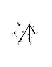
Figure 1: A regular hexagon of interacting qubits

where $S_{i}^{+}$ and $S_{i}^{-}$ are the raising and lowering operators of qubit $i$. The sole assumption we make regarding the interaction potential $\Omega_{ij}$ is that it is a function only of the separation between qubits $i$ and $j$, ${\bf r}_{ij}={\bf r}_{i}-{\bf r}_{j}$. We focus in this paper on qubits arranged at the vertices of regular polygons, and number them sequentially around the polygon (see Fig. 1). For nearest-neighbour qubits, we define $\Omega_{i,i\pm 1}=a$; similarly, $\Omega_{i,i\pm 2}=b$; for $N$ atoms there are $\lfloor N/2\rfloor$ characteristic interactions, which we label sequentially alphabetically.

In analysing the system of interacting qubits we are faced with two possibilities; in this paper we follow option (ii):

(i) We can take the $\Omega_{ij}$ to be real, for example equal to the well known expression for the dipole-dipole interaction energy. Diagonalizing the interaction Hamiltonian yields eigenvalues which are the energy level shifts. The dynamics of the system can then be analyzed using a master equation, which would include terms containing the dipole-dipole damping. By solving the master equation we can calculate various quantities of interest, in particular the total decay rate from a given eigenstate to all the states below it; this is useful for identifying long lived states desirable for quantum computing.

(ii) Alternatively, we can include the free-atom radiation damping $H_{d}=\sum_{i=1}^{N}\hbar\gamma|1_{i}\rangle\langle 1_{i}|$, and as well take the $\Omega_{ij}$ to be complex. The real part of $\Omega_{ij}$ is then the interaction energy, the imaginary part the inter-qubit damping. Although this results in a non-Hermitian Hamiltonian, it has the advantage that the imaginary part of each resulting eigenvalue automatically contains the total decay rate for that eigenstate (the real part is still the energy shift). This is proven elsewhere [hsfII] ; [17] .

The full Hamiltonian to be diagonalized is represented by a $2^{N}\times 2^{N}$ matrix. Fortunately, it is block-diagonal in structure, breaking up into a series of submatrices, in each of which the coupled subsets of states all have the same number $n$ of excited qubits. The submatrices are of dimension $N\choose n$, and the submatrix for $n$ excited qubits is the same as that for $N-n$ excited, a general property of exchange interactions; this halves the amount of work we must do (and we consequently tabulate results only for $n=1,\ldots,\lfloor\frac{N}{2}\rfloor$). The $n=0$ and $n=N$ eigenstates are just $|G\rangle$ and $|E\rangle$ respectively.

I.1 $n=1:$ Single excitation eigenstates

The single excitation (or $n=1$) eigenstates of a system of $N$ qubits arranged at the vertices of a regular polygon were calculated years ago [hsfIII] , guided by the symmetry of the system under rotation about an axis perpendicular to the polygon plane; the $n=1$ eigenvalues and eigenstates for $N=1-6$ are there tabulated. Here we rewrite these calculations in a notation which allows us to extend them to states containing higher numbers of excited qubits, using the case of $N=5$ as an example.

In the subspace spanned by the basis vectors $\{|1\rangle,|2\rangle,\cdots,|5\rangle\}$, the matrix to be diagonalized has the form

$$H_{int}^{(1)}=\left(\begin{array}[]{ccccc}0&a&b&b&a\\ a&0&a&b&b\\ b&a&0&a&b\\ b&b&a&0&a\\ a&b&b&a&0\end{array}\right).$$

We introduce the matrix $P$, a generator of the 5-dimensional representation of $C_{5}$ (the cyclic group of order 5):

$$P=\left(\begin{array}[]{ccccc}0&1&0&0&0\\ 0&0&1&0&0\\ 0&0&0&1&0\\ 0&0&0&0&1\\ 1&0&0&0&0\end{array}\right).$$ (2)

The eigenvalue equation of $P$ is given by

$$Pu_{(v)}=\lambda^{v}u_{(v)},$$

where $\lambda\equiv e^{{2\pi i}\over 5}$, $u_{(v)}=(\lambda^{v},\lambda^{2v},\lambda^{3v},\lambda^{4v},\lambda^{5v})$, and $v=1,\cdots,5$. We define the polynomial $M(x)=a(x+x^{4})+b(x^{2}+x^{3})$, in terms of which $H_{int}^{(1)}=M(P)$. Since $H_{int}^{(1)}$ is a sum of powers of $P$, the eigenvectors $u_{(v)}$ of $P$ will be eigenvectors of $H_{int}^{(1)}$ as well, and we write the eigenvalue equation

$$H_{int}^{(1)}u_{(v)}=m_{(v)}u_{(v)},$$

where the eigenvalues $m_{(v)}=M(\lambda^{v})\equiv G_{(v)}^{(1)}+iF_{(v)}^{(1)}$. There is 1 non-degenerate eigenvalue corresponding to $v=5$, $m_{(5)}=2a+2b$, and (5-1)/2 degenerate pairs of eigenvalues, corresponding to roots which are complex conjugates of each other: $\lambda^{v}=(\lambda^{5-v})^{*}$. The eigenvector corresponding to $m_{(5)}$ is simply $u_{(5)}=(1,1,1,1,1)$. For the eigenvectors corresponding to the degenerate pairs of eigenvalues, we choose the real linear combinations of $u_{(v)}$ and $u_{(5-v)}$,

$$RU_{(v)} = {1\over 2}(u_{(v)}+u_{(5-v)})$$ (3)

$$IU_{(v)} = {1\over{2i}}(u_{(v)}-u_{(5-v)}).$$ (4)

Together with $u_{(5)}$, these form an orthogonal basis set for the $n=1$ subspace. They are listed in Table II.

I.2 $n=2$: Double excitation eigenstates

I.2.1 Odd values of N

We continue with the example of $N=5$ to demonstrate how to calculate the $n=2$ (biexciton) eigenstates for general odd values of $N$. The subspace corresponding to $N=5$, $n=2$ has 10 basis states, which we take in the order $\{|12\rangle,|23\rangle,\cdots,|51\rangle;|13\rangle,|24\rangle,\cdots,|52\rangle\}$.

If we define the four polynomials $M_{11}(x)=b(x+x^{4})$, $M_{12}(x)=a(x^{4}+x^{5})+b(x+x^{3})$, $M_{21}(x)=a(x+x^{5})+b(x^{2}+x^{4})$ and $M_{22}(x)=a(x^{2}+x^{3})$, then the interaction can be represented by the $10\times 10$ matrix,

$$H_{int}^{(2)}=M(P)\equiv\left(\begin{array}[]{cc}M_{11}(P)&M_{12}(P)\\ M_{21}(P)&M_{22}(P)\end{array}\right).$$

Thus, $H_{int}^{(2)}$ is partitioned into a $2\times 2$ array of square submatrices, each of dimension $5\times 5$. The ability to write the matrix in this form is directly due to the ordering of the basis vectors, which allows the rotational symmetry of the pentagon to be reflected in each of the submatrices. It is easy to show that for any odd value of $N$, $H_{int}^{(2)}$ can be partitioned in this way into an array of $(N-1)/2\times(N-1)/2$ square submatrices, each of dimension $N\times N$. This results in a dramatic simplification of the problem, for instance here we need diagonalize only a 2-dimensional matrix instead of the original 10-dimensional one.

As with the $n=1$ case discussed above, each matrix $M_{ij}(P)$ is a linear combination of $P$ and its powers, and therefore has the eigenvalue equation

$$M_{ij}(P)u_{(v)}=M_{ij}(\lambda^{v})u_{(v)},$$

where $\lambda^{v}$ and $u_{(v)}$ are the eigenvalues and eigenvectors of $P$. In order to obtain the eigenvalues and eigenvectors of $H_{int}^{(2)}$, we first solve the eigenvalue equation

$$M(x)V(x)=\mu(x)V(x),$$

where $V(x)$ is an eigenvector and $\mu(x)$ an eigenvalue of the two-dimensional matrix $M(x)$. The solutions are easily found to be

$$\mu^{\pm}(x)={1\over 2}\big{[}M_{11}(x)+M_{22}(x)\pm R(x)\big{]},$$

where

$$R(x)=\sqrt{\big{(}M_{11}(x)-M_{22}(x)\big{)}^{2}+4M_{12}(x)M_{21}(x)},$$

and

$$V^{\pm}(x)=\left(\begin{array}[]{c}M_{11}(x)-M_{22}(x)\pm R(x)\\ 2M_{21}(x)\end{array}\right).$$

The eigenvalues and eigenvectors of $H_{int}^{(2)}$ can then be shown by direct substitution to be $\{\mu^{\pm}(\lambda^{v})\}$ and

$$U^{\pm}_{(v)}=V^{\pm}(\lambda^{v})\otimes u_{(v)}=\left(\begin{array}[]{c}V_{1}^{\pm}(\lambda^{v})u_{(v)}\\ V_{2}^{\pm}(\lambda^{v})u_{(v)}\end{array}\right),$$

where $v=1,\cdots,5$. As with $n=1$, for degenerate eigenvalues we form the real linear combinations of the eigenvectors; the complete orthogonal basis set is listed in Table II.

In general, the eigenvalue equation for the $n=2$ excitations of any odd-$N$ array of qubits is solved in the same way:

(i) The interaction matrix $H_{int}^{(2)}$ is partitioned into an array of square submatrices, each of dimension $N\times N$.

(ii) The eigenvalue equation of matrix $M_{ij}(P)$ is solved, where $P$ is the $N\times N$ matrix analogous to Eq.(2).

(iii) The eigenvalue equation is solved for the corresponding $(N-1)/2\times(N-1)/2$ matrix $M(x)$, yielding eigenvalues $\{\mu_{(i)}(x)\}$ and eigenvectors $\{V_{(i)}(x)\}$.

(iv) The eigenvalues and eigenvectors of $H_{int}^{(2)}$ are then given by $\{\mu_{(i)}(\lambda^{v})\equiv G_{(vi)}^{(2)}+iF_{(vi)}^{(2)}\}$ and $\{U_{(vi)}=V_{(i)}(\lambda^{v})\otimes u_{(v)}\}$, where $v=1,\cdots,N$, $i=1,\cdots,\lfloor(N-1)/2\rfloor$, $\lambda=e^{\frac{2\pi i}{N}}$, and the vectors $\{u_{(v)}\}$ are the eigenvectors of the matrix $P$ corresponding to the $N$-sided polygon.

I.2.2 Even values of $N$

The calculations for the $n=2$ energies and eigenstates for even values of $N$ cannot be described (or performed) so succinctly. This is due to the fact that $(N-1)/2$ is an odd half-integer. As a result, the matrix for $H_{int}^{(2)}$ consists of 2 parts: an inner “core” of $\lfloor(N-1)/2\rfloor\times\lfloor(N-1)/2\rfloor$ square submatrices, each of dimension $N\times N$, plus an outer section of $N/2$ extra columns to the right and rows at the bottom of the core. For example, the $n=2$ interaction matrix for $N=4$ is given by

$$H_{int}^{(2)}=\left(\begin{array}[]{cccc|cc}0&b&0&b&a&a\\ b&0&b&0&a&a\\ 0&b&0&b&a&a\\ b&0&b&0&a&a\\ \hline\cr a&a&a&a&0&0\\ a&a&a&a&0&0\\ \end{array}\right),$$

with an inner core matrix $M(P)=b(P+P^{3})$, where $P$ is now the 4-dimensional analogue of Eq.(2).

The calculations are performed in the following manner; we illustrate the general procedure with the example of $N=4$:

(i) The energy eigenvalues and vectors of the “core” matrix are obtained, in exactly the same way as described in the previous section for odd values of $N$.

For the case of $N=4$, the eigenvectors of $M(P)$ are the same as those of $N=4,n=1$, which in turn are the same as those of $P$. They appear in Table 1.

(ii) These eigenvectors are then divided into 2 groups, according to their symmetry or antisymmetry. The vectors $(1,1,\cdots,1,1)$ and $(1,-1,1,-1,\cdots,1,-1)$ are always eigenvectors, the former symmetric, the latter antisymmetric; the remainder are classified according to their symmetry under rotations of $\pi$ about the symmetry axis.

In the case of $N=4$, three of these eigenvectors (those corresponding to $v=1,2,\text{ and }3$ as listed in Table 1) are antisymmetric, while that corresponding to $v=4$ is symmetric.

(iii) The antisymmetric eigenvectors are appended with $N/2$ $0$’s; the resulting vectors are eigenvectors of $H_{int}^{(2)}$, and the corresponding energies are found by direct substitution.

In the case of $N=4$, by appending two $0$’s to the ends of the antisymmetric vectors, we obtain the following three eigenvectors of $H_{int}^{(2)}$:

$$U_{(1)}=\left(\begin{array}[]{c}1\\ 0\\ -1\\ 0\\ 0\\ 0\end{array}\right),\;U_{(2)}=\left(\begin{array}[]{c}-1\\ 1\\ -1\\ 1\\ 0\\ 0\end{array}\right),\;U_{(3)}=\left(\begin{array}[]{c}0\\ 1\\ 0\\ -1\\ 0\\ 0\end{array}\right).$$

The corresponding eigenvalues are found by substitution. By symmetry, we see that a fourth (antisymmetric) eigenvector of $H_{int}^{(2)}$ is $U=(0,0,0,0,1,-1)$.

(iv) The symmetric eigenvectors are extended into the rest of the $n=2$ subspace in a symmetric fashion.

For the example of $N=4$, the remaining 2 eigenvectors are found from the symmetric eigenvector $u_{(4)}=(1,1,1,1)$ of $H_{int}^{(1)}$. We substitute into the eigenvalue equation for $H_{int}^{(2)}$ the trial vector $U=(1,1,1,1,x,x)$, obtaining 2 (independent) equations for $x$ and the eigenvalues $\mu$: $2b+2ax=\mu$ and $4a=\mu x.$ These have the solutions $\mu^{\pm}=b\pm R,$ $x^{\pm}={4a\over{b\pm R}}$, where $R=\sqrt{b^{2}+8a^{2}}$. This completes our set of 6 eigenvectors of $H_{int}^{(2)}$. They are listed together with their corresponding eigenvalues in Table 1 .

We point out that the $N=4$, $n=2$ eigenstates are the first which depend on the actual strength of the interaction, and not merely on its symmetry. In Fig. 2, we illustrate the distance dependence of their decay rates. In the long-wavelength limit , three of the eigenstates have their decay rates unchanged from the noninteracting value of $2\gamma$, and one state is superradiant, with an asymptotic value of $5.930\gamma$ (see Table V). The remaining two states are subradiant: One shows weak optical activity, with a limiting decay rate of $0.070\gamma$, and one is completely subradiant, with decay rate $\rightarrow 0$; thus, this state is of possible interest for the encoding of quantum information. (We have cut off the figure at $\lambda/r=10$ in order to retain the visibility of some of the oscillations at low values of the argument, corresponding to shorter wavelengths.)

I.3 Triple excitation eigenstates

To complete the sets of eigenstates for the $N=6$ and $N=7$ polygons, we require those corresponding to the $n=3$ excitations. These are obtained with methods very similar to those used for the $n=2$ states. For $N=7$, the $H_{int}^{(3)}$ matrix is first partitioned into a $5\times 5$ array of square submatrices, each of dimension $7\times 7$. The solution then requires the (preliminary) diagonalization of a $5\times 5$ matrix $M(P)$, but is otherwise a direct extension of the method used for $n=2$.

For $N=6$ we choose the basis vectors in the order: $\{|123\rangle,|234\rangle,\cdots,|612\rangle;$ $|124\rangle,|235\rangle,\cdots,|613\rangle;$ $|134\rangle,|245\rangle,\cdots,|623\rangle;$ $|135\rangle,|246\rangle\}$. Doing so we find that the matrix $H_{int}^{(3)}$ consists of a core array of $3\times 3$ submatrices, each of dimension $6\times 6$, together with an outer section of 2 columns to the right and 2 rows at the bottom of the core. The solution consists of 2 stages: In the first stage, the eigenvalues and eigenvectors of the core matrix are found, and in the second the symmetric and antisymmetric eigenvectors of the core are extended to become those of the full $20\times 20$ matrix, in a manner entirely analogous to that employed for $N=6$, $n=2$. The complete set of eigenvalues and eigenvectors for N=6 is listed in Table III. Those for N=7 are available upon request.

II COOPERATIVE RADIATIVE TRANSITIONS

In this section, we focus on systems of identical two-level atoms (or molecular monomers) undergoing cooperative radiative transitions; the interatomic potential which applies in this case is the retarded multipole-multipole interaction [12] . The strongest and most common of these are 1-photon transitions due to the electric dipole moment operator; however, the same analysis can also be made for magnetic dipole or (with different $\Omega_{ij}$) higher electric multipole transitions [hsfI] ; [12] ; [13] as well, and even for 2-photon transitions [2p] . We point out that in many systems an interaction exists between nearest neighbours (e.g. due to atomic overlap) in addition to the electromagnetic exchange interaction which occurs between all pairs. These forces can be included trivially in our analysis, simply by incorporating them into the nearest-neighbour interaction $\Omega_{i,i\pm 1}=a$.

For the simple case of linear transition dipoles, of transition strength $\mu$, oriented (parallel to each other and) perpendicular to the plane of the ring, $\Omega_{ij}$ can be written in the form

$$\Omega_{ij}=i\gamma\biggl{[}-{1\over 2}h_{2}^{(2)}(kr_{ij})+h_{0}^{(2)}(kr_{ij})\biggr{]},$$

where $h_{n}^{(2)}$ is a spherical Hankel function of the second kind [14] and $\gamma$ is half the atomic Einstein $A$ coefficient,

$$\gamma={{2|\mu|^{2}\omega^{3}}\over{3\hbar c^{3}}}.$$

For linear transition quadrupoles oriented perpendicular to the plane of the ring, the interaction is

$$\Omega_{ij}=i\gamma_{q}\biggl{[}-{9\over 28}h_{4}^{(2)}(kr_{ij})+{5\over 28}h_{2}^{(2)}(kr_{ij})+{1\over 2}h_{0}^{(2)}(kr_{ij})\biggr{]},$$

where $\gamma_{q}$ is half the Einstein $A$ coefficient for the (quadrupole) transition,

$$\gamma_{q}={{|q|^{2}\omega^{5}}\over{15\hbar c^{5}}}$$

[hsfI] ; [13] . However, the analysis is also valid for any system in which the transition moments of all identical units are oriented symmetrically, i.e. they form the same angle with the ring. For example, there exist molecular aggregates in biology known as “light-harvesting complexes”, in which large identical building blocks or monomers are arranged symmetrically in rings with an N-fold symmetry axis, whose electronic excitations have been found to extend coherently over the entire ring [15] . The direction of the transition moment of each individual monomer forms the (same small) angle $\theta\neq 90^{o}$ with the tangent to the ring at its position. In this case, the dipole-dipole interaction is (slightly) more complicated in form, and is given by

$$\Omega_{ij}=i\gamma\bigg{[}{1\over 2}\bigl{\{}3(\hat{\mu}_{i}\cdot\hat{\bf r}_{ij})(\hat{\mu}_{j}\cdot\hat{\bf r}_{ij})-\hat{\mu}_{i}\cdot\hat{\mu}_{j}\bigr{\}}h_{2}^{(2)}(kr_{ij})+(\hat{\mu}_{i}\cdot\hat{\mu}_{j})\,h_{0}^{(2)}(kr_{ij})\bigg{]},$$

but all our calculations remain valid.

The dynamics of the system are governed by the Lehmberg-Agarwal master equation [16] , which may be solved by projection onto any complete set of basis vectors. However, the “natural” set for this projection are the eigenstates of the Hamiltonian $H=H_{f}+H_{d}+H_{int}$. As demonstrated previously for $N=2$ and $3$ [hsfII] and elsewhere for general $N$ [17] , these states have the following properties:

1. The real part of the (complex) eigenvalue gives the shift of energy of the exciton due to local field effects.

2. The imaginary part of the eigenvalue gives the total decay rate or inverse lifetime of the state; this total decay rate is the sum of the individual decay rates to all states in the energy manifold below, as calculated using the master equation and in agreement with the total energy radiated by the system in a transition between the two states [17] .

3. The eigenstates form the basis set within which the population dynamics and spectroscopic properties of the system are most conveniently studied.

A calculation of the $n=1$ and $n=2$ eigenstates of regular polygon systems of odd $N$ for electric dipole interactions in the long-wavelength limit has in fact been carried out [muk] , but in that reference the authors included only nearest-neighbour coupling for the real part of the interaction. For the $n=1$ subspace, the resulting eigenstates are the same as ours (which however include interactions between all neighbours and are valid for arbitrary wavelength), but the energies are very different: This difference is illustrated in Table 4, where we list the $n=1$ energies in the long-wavelength limit for polygons having $N=5$ and $N=6$, for nearest-neighbour interactions only, for linear dipoles with all neighbours included, and for linear quadrupoles with all neighbours included. (All energies are expressed in units of the static interaction energy $V_{N}$ between a pair of nearest neighbours.) For the $n=2$ subspace, the eigenstates themselves are very different from those obtained when only nearest-neighbour interactions are included, and a numerical comparison of the energies is not meaningful. Because the retarded interactions are intrinsically long-ranged, a correct calculation of the eigenstates of the physical system must include interactions between all atom pairs: Only in these states will the “local field” shifts be the same, and only in these states will the damping be the same for all atoms, so that no dephasing occurs during the evolution in time [18] . As well, in some systems the energy of interaction between second (or higher) nearest neighbours can actually exceed that between adjacent pairs (depending on the relative phases of the moments in the given eigenstate, and/or on the relative orientations of the transition moments and ${\bf r}_{ij}$).

The detailed emissive properties of these systems will be presented elsewhere [17] ; however, some simple properties are immediately evident in the eigenvalues and eigenvectors. For example, in the long wavelength limit only one $n=1$ state is optically active in absorption and emission, and it is superradiant, having an eigenvalue whose imaginary part $\rightarrow N\gamma$; the $N-1$ other single-excitation states are subradiant, with the imaginary parts of their eigenvalues $\rightarrow 0$. In general, the $n=2$ states decay into $n=1$ states (although these in turn may be subradiant); however, for even-$N$ polygons, there is (at least) one $n=2$ state which is itself completely subradiant.

As a simple illustration of the emissive pattern, in Fig. 2 we display a complete energy level diagram for $N=3$ [footnote] . All atomic separations are equal, so that the system is described by a single interaction potential $a=\gamma(g+if)$. On each state is indicated its total decay rate, while individual decay rates between states are indicated on the dashed lines connecting them. For example, the $n=2$ eigenstate $(1,\ 1,\ 1)$ has energy $\hbar(2\omega+2\gamma g)$ and a total decay rate of $2\gamma(1+f)$; it decays at a rate of $\gamma(4+8f)/3$ to the (symmetric) $(1,\ 1,\ 1)$ state, and at a rate of $\gamma(1-f)/3$ to each of the 2 antisymmetric states in the $n=1$ manifold below it. Similarly, each of the other two $n=2$ eigenstates has energy $\hbar(2\omega-\gamma g)$ and a total decay rate of $\gamma(2-f)$. The small sample/long wavelength limit corresponds to $f\rightarrow 1$. In this limit, all the $n=2$ eigenstates decay, but the two antisymmetric $n=1$ states are (completely) subradiant.

II.1 Absorption from an external field

If a system in its ground state is placed in a weak external field of wave vector ${\bf k}$ and polarization $\hat{\bf e}_{\lambda}$, only the $n=1$ states are excited, with a relative probability proportional to $|\langle u_{(v)}|\sum_{i}\,S_{i}^{+}\vec{\mu}\cdot\hat{\bf e}_{\lambda}\,e^{i{\bf k}\cdot{\bf R}_{i}}|G\rangle|^{2}$. If the field is sufficiently intense and the losses sufficiently low, population can remain in the $\{u_{(v)}\}$ states for long enough to allow excitation of the $n=2$ states; and so on.

In recent years, there has been interest in the excitation of the exciton and biexciton states of the light-harvesting complexes, in connection with the calculation of their third-order nonlinear optical susceptibilities [muk] . The complexes discovered so far have diameters of the order of 10 nm, and their absorption frequencies correspond typically to wavelengths $\geq 400$ nm, so that the long-wavelength limit applies. In this limit, the dependence on ${\bf k}$ in the absorption probability is negligible, and it is easy to verify that only those states $\{u_{(v)}\}$ which are totally symmetric in the atomic positions are optically active, namely the states $u_{(N)}=(1,\cdots,1)$. This gives rise to lorentzian (exciton) absorption lines, centred at the shifted frequencies $G_{(N)}^{(1)}\equiv\omega_{0}+\Delta G_{(N)}^{(1)}$, with (natural) widths $2F_{(N)}^{(1)}=2N\gamma$.

We denote the energy of state $U_{(vi)}$ by $G_{(vi)}^{(2)}=2\omega_{0}+\Delta G_{(vi)}^{(2)}$, and its decay constant by $F_{(vi)}^{(2)}$. The excitation of state $U_{(vi)}$ from a ring in the state $u_{(N)}$ then occurs at frequency $G_{(vi)}^{(2)}-G_{(N)}^{(1)}$. It can be shown [17] that the width of the absorption line is $2(F_{(vi)}^{(2)}+F_{(N)}^{(1)})$, and that in the long-wavelength limit the relative intensities of the biexciton absorption lines are simply given by $F_{(vi)}^{(2)}$.

In Table V we list the $n=1$ shifts $\Delta G_{(N)}^{(1)}$, the (unnormalized) $n=2$ eigenvectors $\{U_{(vi)}\}$, and the $n=2$ shifts $\Delta G_{(vi)}^{(2)}$ and decay constants $F_{(vi)}^{(2)}$ for $N=2,\cdots,9$, in the long-wavelength limit. The vectors $\{U_{(vi)}\}$ correspond to basis states arranged in the order $\{|12\rangle,|23\rangle,\cdots,|N1\rangle;|13\rangle,|24\rangle,\cdots,|N2\rangle;\ etc\}$. In Table VI we list the corresponding biexciton excitation frequency shifts, (natural) half widths, and relative intensities. All frequencies are expressed in units of $V_{N}$, and widths in units of $\gamma$.

III CONCLUSIONS

We have calculated the eigenstates corresponding to coherent single and multiple excitations of an array of $N$ identical TLA’s or qubits arranged on the vertices of a regular polygon. Their coupling occurs via an exchange interaction which depends only on the separation between the qubits. We include the interactions between all pairs, and our results are valid for arbitrary distances relative to the radiation wavelength. To illustrate the usefulness of these eigenstates, we plot the distance dependence of the decay rates of the $n=2$ eigenstates of a system of 4 qubits arranged on the vertices of a square, and tabulate the biexciton eigenstates and eigenvalues, and absorption frequencies, line widths, and relative intensities for polygons of $N=2,\cdots,9$ identical TLA’s, in the long-wavelength limit. The states will be used elsewhere to study the emissive properties of these systems [17] and to calculate the amount and distribution of entanglement in these “natural” entangled states at both zero and finite temperature.

References

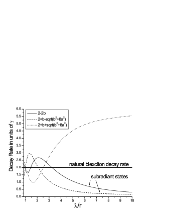
Figure 2: Distance dependence of the decay rates of the $N=4,n=2$ eigenstates

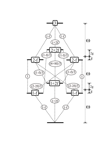
Figure 3: Energy levels and decay rates for an equilateral triangle of qubits (in units of the single qubit decay rate); $g$ ($f$) is the real (imaginary) part of the inter-qubit potential $a$.

$N$	$n$	$v$	Eigenvalues	Eigenvectors
2	1	1	$-a$	$(-1,1)$
		2	$a$	$(1,1)$
3	1	1,2	$-a$	$(-1,-1,2);(1,-1,0)$
		3	$2a$	$(1,1,1)$
4	1	1,3	$-b$	$(0,-1,0,1);(1,0,-1,0)$
		2	$-2a+b$	$(-1,1,-1,1)$
		4	$2a+b$	$(1,1,1,1)$
	2	1,3	$0$	$(0,-1,0,1,0,0);(1,0,-1,0,0,0);(0,0,0,0,1,-1)$
		2	$-2b$	$(-1,1,-1,1,0,0)$
		4	$b\pm R$	(1,1,1,1,$x_{\pm},x_{\pm}$)
			$R=\sqrt{b^{2}+8a^{2}}$    $x_{\pm}=(-b\pm R)/2a$

Table 1: Eigenvalues and eigenvectors of a single pair (N=2), equilateral triangle (N=3), and square array (N=4) of qubits.

$n$	$v$	Eigenvalues	Eigenvectors
1	1,4	$2(c_{2}a-c_{1}b)$	$(c_{2},c_{4},c_{6},c_{8},c_{10});(s_{2},s_{4},s_{6},s_{8},s_{10})$
	2,3	$2(-c_{1}a+c_{2}b)$	$(c_{4},c_{8},c_{12},c_{16},c_{20});(s_{4},s_{8},s_{12},s_{16},s_{20})$
	5	$2a+2b$	(1,1,1,1,1)
2	1,4	$E_{\pm}(-c_{1}a,c_{2}b)$	$(c_{2},-c_{1},-c_{1},c_{2},1;v_{\pm}c_{2},v_{\pm},v_{\pm}c_{2},-v_{\pm}c_{1},-v_{\pm}c_{1})$
			$(-1,-2c_{2},2c_{2},1,0;v_{\pm},0,-v_{\pm},-2v_{\pm}c_{2},2v_{\pm}c_{2})$
	2,3	$E_{\pm}(c_{2}a,-c_{1}b)$	$(-c_{1},c_{2},c_{2},-c_{1},1;-w_{\pm}c_{1},w_{\pm},-w_{\pm}c_{1},w_{\pm}c_{2},w_{\pm}c_{2})$
			$(-2c_{2},1,-1,2c_{2},0;2w_{\pm}c_{2},0,-2w_{\pm}c_{2},w_{\pm},-w_{\pm})$
	5	$E_{+}(a,b)$	$(1,1,1,1,1;u,u,u,u,u)$
		$E_{-}(a,b)$	$(u,u,u,u,u;-1,-1,-1,-1,-1)$
	$\begin{array}[]{rclrcl}c_{j}&=&\cos(j\pi/5)&u&=&G_{+}(a,b)\\ s_{j}&=&\sin(j\pi/5)&v_{\pm}&=&G_{\pm}(-c_{1}a,c_{2}b)\\ F(\alpha,\beta)&=&\sqrt{5(\alpha+\beta)^{2}-4\alpha\beta}&w_{\pm}&=&G_{\pm}(c_{2}a,-c_{1}b)\\ E_{\pm}(\alpha,\beta)&=&\alpha+\beta\pm F(\alpha,\beta)&G_{\pm}(\alpha,\beta)&=&[\alpha-\beta\pm F(\alpha,\beta)]/2(\alpha+\beta)\end{array}$

Table 2: Eigenvalues and eigenvectors of 5 qubits arranged on the vertices of a regular pentagon.

$n$	$v$	Eigenvalues	Eigenvectors
1	1,5	$a-b-c$	$(1,-1,-2,,-1,,1,2);(1,1,0,-1,-1,0)$
	2,4	$-a-b+c$	$(-1,-1,2,-1,-1,2);(1,-1,0,1,-1,0)$
	3	$-2a+2b-c$	$(-1,1,-1,1,-1,1)$
	6	$2a+2b+c$	$(1,1,1,1,1,1)$
2	1,5	$\pm\sqrt{b^{2}+3a^{2}}$	$(1,-1,-2,-1,1,2;0,-u_{\pm},-u_{\pm},0,u_{\pm},u_{\pm};0,0,0)$
			$(3,3,0,-3,-3,0;2u_{\pm},u_{\pm},-u_{\pm},-2u_{\pm},-u_{\pm},u_{\pm};0,0,0)$
	2,4	$\nu$	$(-1,-1,2,-1,-1,2;-2x,x,x,-2x,x,x;-y,2y,-y)$
			$(1,-1,0,1,-1,0;0,-x,x,0,-x,x;-y,0,y)$
	3	$-2b$	$(-1,1,-1,1,-1,1;0,0,0,0,0,0;0,0,0)$
		$2b$	$(0,0,0,0,0,0;-1,1,-1,1,-1,1;0,0,0)$
	6	$\mu$	$(1,1,1,1,1,1;r,r,r,r,r,r;s,s,s)$
		$\small\begin{array}[]{c}\begin{array}[]{rclrcl}\\[-8.0pt] \nu^{3}+2b\nu^{2}+(4ac-b^{2}-3a^{2}-4c^{2})\nu+2b(b^{2}-a^{2}+4ac)&=&0&\;\;x&=&(\nu^{2}+b\nu-2b^{2})/[\nu(a-2c)-2ab]\\ \mu^{3}-4b\mu^{2}-4(2ac+b^{2}+3a^{2}+c^{2})\mu+16b(b^{2}-a^{2}-2ac)&=&0&\;\;y&=&2(a\nu+2bc)/[\nu(a-2c)-2ab]\\ \end{array}\\ r=(\mu^{2}-2b\mu-8b^{2})/2[\mu(a+c)+4ab]\;\;\;\;\;\;s=2(a\mu+2bc)/[\mu(a+c)+4ab]\;\;\;\;\;\;u_{\pm}=-b\pm\sqrt{b^{2}+3a^{2}}\end{array}$
3	1,5	$a-b-c+(a+b)m_{\pm}$	$(m_{\pm},-m_{\pm},-2m_{\pm},-m_{\pm},m_{\pm},2m_{\pm};1,-1,-2,-1,1,2;-1,-2,-1,1,2,1;0,0)$
			$(m_{\pm},m_{\pm},0,-m_{\pm},-m_{\pm},0;1,1,0,-1,-1,0;1,0,-1,-1,0,1;0,0)$
	$1,5\atop 2,4$	$b\mp a\mp c$	$(0,0,0,0,0,0;-2,\mp 1,1,\pm 2,1,\mp 1;\pm 1,-1,\mp 2,-1,\pm 1,2;0,0)$
			$(0,0,0,0,0,0;0,-1,\mp 1,0,\pm 1,1;1,\pm 1,0,\mp 1,-1,0;0,0)$
	2,4	$c-a-b+(a-b)n_{\pm}$	$(n_{\pm},n_{\pm},-2n_{\pm},n_{\pm},n_{\pm},-2n_{\pm};1,1,-2,1,1,-2;1,-2,1,1,-2,1;0,0)$
			$(n_{\pm},-n_{\pm},0,n_{\pm},-n_{\pm},0;1,-1,0,1,-1,0;-1,0,1,-1,0,1;0,0)$
	3	$\sigma_{-}$	$(-p_{-},p_{-},-p_{-},p_{-},-p_{-},p_{-};1,-1,1,-1,1,-1;-1,1,-1,1,-1,1;-q_{-},q_{-})$
	$3\atop 6$	$\mp c\pm 2a-2b$	$(0,0,0,0,0,0;\mp 1,1,\mp 1,1,\mp 1,1;-1,\pm 1,-1,\pm 1,-1,\pm 1;0,0)$
	6	$\sigma_{+}$	$(p_{+},p_{+},p_{+},p_{+},p_{+},p_{+};1,1,1,1,1,1;1,1,1,1,1,1;q_{+},q_{+})$
		$\begin{array}[]{rcl}\\[-8.0pt] \sigma_{\pm}^{3}&-&(2b\pm 3c\pm 2a)\sigma_{\pm}^{2}-[4(a^{2}+b^{2})+(2a\pm 2b-c)^{2}]\sigma_{\pm}\pm 3c[c^{2}+2(\pm bc\mp 4ab+ac)]=0\\ p_{\pm}&=&2[\left(2b\pm a\right)\sigma_{\pm}+3ca]/[\sigma^{2}_{\pm}\mp 2c\sigma_{\pm}-3c^{2}]\\ q_{\pm}&=&6[a\sigma_{\pm}\mp ac+2bc]/[\sigma^{2}_{\pm}\mp 2c\sigma_{\pm}-3c^{2}]\\ m_{\pm}&=&[{{2c+b-a\pm\sqrt{(2c+b-a)^{2}+8(a+b)^{2}}}]/[{2(a+b)}}]\\ n_{\pm}&=&[{{a+b-2c\pm\sqrt{(2c-b-a)^{2}+8(a-b)^{2}}}]/[{2(a-b)}}]\end{array}$

Table 3: Eigenvalues and eigenvectors of 6 qubits arranged on the vertices of a regular hexagon.

$N$	$v$	Energy	nearest neighbours	linear dipoles,	linear quadrupoles,
			only	all neighbours	all neighbours
5	1, 4	$.618a-1.618b$	.618	.239	.474
	2, 3	$-1.618a+.618b$	$-1.618$	$-1.473$	$-1.563$
	5	$2a+2b$	2	2.468	2.178
6	1, 5	$a-b-c$	1	.683	.905
	2, 4	$-a-b+c$	$-1$	$-1.067$	$-1.033$
	3	$-2a+2b-c$	$-2$	$-1.741$	$-1.902$
	6	$2a+2b+c$	2	2.509	2.159

Table 4: $n=1$ energies in the small sample limit (units of the static interaction energy between nearest neighbours).

$N$	$\Delta G_{(N)}^{(1)}$	$n=2$ eigenvectors	$\Delta G_{(vi)}^{(2)}$	$F_{(vi)}^{(2)}$
	(units of $V_{N}$)		(units of $V_{N}$)	(units of $\gamma$)
2	1	$(1)$	0	2
3	2	$(1,1,1)$	2	4
4	2.354	$(1,1,1,1,x,x)$
		$x=1.248-.283i/V_{N}$	3.204	5.930
		$x=-1.602-.363i/V_{N}$	-2.496	.070
5	2.472	$(1,1,1,1,1;x,x,x,x,x)$
		$x=1.356+.649i/V_{N}$	3.823	7.821
		$x=-.737-.352i/V_{N}$	-1.351	.179
6	2.511	$(1,1,1,1,1,1;x,x,x,x,x,x;y,y,y)$
		$x=1.417-1.261i/V_{N};\ y=1.548-1.732i/V_{N}$	4.162	9.687
		$x=-.114-.373i/V_{N};\ y=-1.087-.550i/V_{N}$	-.290	.293
		$x=-1.940-.312i/V_{N};\ y=2.252+.200i/V_{N}$	-3.100	.020
7	2.518	$(1,1,1,1,1,1,1;x,x,x,x,x,x,x;y,y,y,y,y,y,y)$
		$x=1.45-1.602i/V_{N};\ y=1.66-2.738i/V_{N}$	4.358	11.534
		$x=.314-.433i/V_{N};\ y=-.877-.765i/V_{N}$	.570	.410
		$x=-1.416-.379i/V_{N};\ y=.634+.011i/V_{N}$	-2.410	.056
8	2.515	$(x,x,x,x,x,x,x,x;1,1,1,1,1,1,1,1;y,y,y,y,y,y,y,y;z,z,z,z)$
		$x=0+59.68i/V_{N};\ y=1.177-.949i/V_{N};\ z=1.237-1.444i/V_{N}$	4.478	13.37
		$x=1.635+69.72i/V_{N};\ y=0-.0714i/V_{N};\ z=-1.809-132.87i/V_{N}$	1.248	.528
		$x=-1.0914-285.8i/V_{N};\ y=.4523+.0204i/V_{N};\ z=-1.284+.453i/V_{N}$	-1.660	.097
		$x=-.490-63.44i/V_{N};\ y=-1.33-43.48i/V_{N};\ z=1.451-34.91i/V_{N}$	-3.322	.008
9	2.508	$(1,1,1,1,1,1,1,1,1;x,x,x,x,x,x,x,x,x;y,y,y,y,y,y,y,y,y;z,z,z,z,z,z,z,z,z)$
		$x=1.493-2.834i/V_{N};\ y=1.793-5.665i/V_{N};\ z=1.939-7.341i/V_{N}$	4.559	15.19
		$x=.822-.583i/V_{N};\ y=-.144-1.184i/V_{N};\ z=-1.015-1.518i/V_{N}$	1.780	.644
		$x=-.496-.429i/V_{N};\ y=-.916-.396i/V_{N};\ z=.713-.0043i/V_{N}$	-.958	.140
		$x=-1.713-.386i/V_{N};\ y=1.538+.177i/V_{N};\ z=-.619-.222i/V_{N}$	-2.874	.025

Table 5: Frequency shifts and widths of the exciton and biexciton energy levels (long-wavelength limit).

$N$	Frequency shifts	Half-widths	Relative Intensities
	(units of $V_{N}$)	(units of $\gamma$)
2	$-1$	4	1
3	0	7	1
4	0.85	9.93	.988
	$-4.85$	4.07	.012
5	1.351	12.821	.978
	$-3.823$	5.179	.022
6	1.651	15.687	.969
	$-2.801$	6.293	.029
	$-5.611$	6.020	.002
7	1.840	18.534	.961
	$-1.948$	7.410	.034
	$-4.929$	7.056	.005
8	1.964	21.370	.9550
	$-1.266$	8.528	.0377
	$-4.174$	8.097	.0069
	$-5.836$	8.008	.0006
9	2.052	24.190	.9494
	$-.727$	9.644	.0403
	$-3.465$	9.140	.0088
	$-5.381$	9.025	.0016

Table 6: Biexciton excitation frequency shifts, natural line widths, and relative intensities (long-wavelength limit).

References

- (1) A. S. Davydov, Theory of Molecular Excitons, (Plenum, New York, 1971); D. P. Craig and S. H. Walmsley, Excitons in Molecular Crystals, (Benjamin, New York, 1968).
- (2) M. Gross and S. Haroche, Physics Reports 93, 301 (1982).
- (3) Francis C. Spano and Shaul Mukamel, Phys. Rev. A40, 5783 (1989); O. Khn and S. Mukamel, J. Phys. Chem. B101, 809 (1997).
- (4) D. Lidar, I. Chuang and K. Whaley, Phys. Rev. Lett. 81, 2594 (1998); H. Matsueda, Superlattices and Microstructures 31, 87 (2002).
- (5) K. O’Connor and W. Wootters, Phys. Rev. A 63, 052302 (2001).
- (6) R. H. Dicke, Phys. Rev. 93, 99 (1954).
- (7) Helen S. Freedhoff, Phys. Rev. A5, 126 (1972).
- (8) A. Crubellier, S. Liberman, D. Pavolini and P. Pillet, J. Phys. B18, 3811 (1985); D. Pavolini, A. Crubellier, P. Pillet, L. Cabaret and S. Liberman, Phys. Rev. Letters 54, 1917 (1985).
- (9) Th Richter, J. Phys. B15, 1293 (1982); Ann. Phys., Lpz 40, 234 (1983).
- (10) Helen S. Freedhoff, J. Phys. B19, 3035 (1986).
- (11) Helen Freedhoff and J. Van Kranendonk, Can. J. Phys. 45, 1833 (1967); M. R. Philpott, J. Chem. Phys. 63, 485 (1975).
- (12) M. R. Philpott and P. G. Sherman, Phys. Rev. B12, 5381 (1975).
- (13) Helen S. Freedhoff, J. Chem. Phys. 85, 6110 (1986).
- (14) H. S. Freedhoff and W. Markiewicz, J. Phys. C13, 5315 (1980); H. S. Freedhoff, J. Phys. C13, 5329 (1980).
- (15) Helen S. Freedhoff, J. Phys. B22, 435 (1989).
- (16) Zhidang Chen and Helen Freedhoff, Phys. Rev A44, 546 (1991).
- (17) G. B. Arfken and H. J. Weber, Mathematical Methods for Physicists, (Harcourt Academic Press, London, 2001).
- (18) Xiche Hu, Thorsten Ritz, Ana Damjanovi and Klaus Schulten, J. Phys. Chem B101, 3854 (1997); Xiche Hu and Klaus Schulten, Physics Today 50, 28 (August, 1997); Herbert van Amerongen, Rienk van Grondelle and Leonas Valkunas, Photosynthetic Excitons, (World Scientific, 2000).
- (19) R. H. Lehmberg, Phys. Rev. A 2, 883 (1970); G. S. Agarwal, Quantum Statistical Theories of Spontaneous Emission and Their Relation to Other Approaches, (Springer, Berlin).
- (20) Itay Yavin and Helen Freedhoff, (to be published).
- (21) B. Coffey and R. Friedberg, Phys. Rev. A17, 1033 (1978).
- (22) A figure identical to this one appears in reference [rich] . In those papers, the author studies the emission from a fully-excited 3-atom system by projecting the master equation onto a basis which consists of the Dicke states [dicke] of the system, rather than the eigenstates of the total hamiltonian. As a consequence, he is able to obtain an analytic solution only when the atoms are arranged to form an equilateral triangle: for this special case (only), the Dicke states coincide with the energy eigenstates. We emphasize that the use of the energy eigenstates always leads to an analytic solution [17] , but we choose the equilateral triangle as an illustration here for its simplicity.