Exact Performance of Concatenated Quantum Codes

Abstract

When a logical qubit is protected using a quantum error-correcting code, the net effect of coding, decoherence (a physical channel acting on qubits in the codeword) and recovery can be represented exactly by an effective channel acting directly on the logical qubit. In this paper we describe a procedure for deriving the map between physical and effective channels that results from a given coding and recovery procedure. We show that the map for a concatenation of codes is given by the composition of the maps for the constituent codes. This perspective leads to an efficient means for calculating the exact performance of quantum codes with arbitrary levels of concatenation. We present explicit results for single-bit Pauli channels. For certain codes under the symmetric depolarizing channel, we use the coding maps to compute exact threshold error probabilities for achievability of perfect fidelity in the infinite concatenation limit.

I Introduction

The methods of quantum error correction Shor (1995); Steane (1996); Nielsen and Chuang (2000) have, in principle, provided a means for suppressing destructive decoherence in quantum computer memories and quantum communication channels. In practice, however, a finite-sized error-correcting code can only protect against a subset of possible errors; one expects that protected information will still degrade, albeit to a lesser degree. The problem of characterizing a quantum code’s performance could thus be phrased as follows: what are the effective noise dynamics of the encoded information that result from the physical noise dynamics in the computing or communication device?

One could address this question by direct simulation of the quantum dynamics and coding procedure. However, for codes of non-trivial size, this approach rapidly becomes intractable. For example, in studies of fault-tolerance Preskill (1997) one often considers families of concatenated codes Knill and Laflamme (1996); Nielsen and Chuang (2000). An $N$-qubit code concatenated with itself $\ell$ times yields an $N^{\ell}$-qubit code, providing better error resistance with increasing $\ell$. For even modest values of $N$ and $\ell$, simulation of the resulting $2^{(N^{\ell})}$-dimensional Hilbert space requires massive computational resources; using simulation to find the asymptotic performance as $\ell\rightarrow\infty$ (as required for fault-tolerant applications) is simply not on option.

Instead, a quantum code is often characterized by the set of discrete errors that it can perfectly correct Knill and Laflamme (1997). For example, the Shor nine-bit code Shor (1995) was designed to perfectly correct arbitrary decoherence acting on a single bit in the nine-bit register. Typical analyses of such codes implicitly assume that the physical dynamics can be described by single-bit errors occurring at some probabilistic rate; if this rate is small (e.g. $O(p)$ for $p\ll 1$), the probability that these errors will accumulate into a multi-bit uncorrectable error is also small (e.g. $O(p^{2})$). This type of leading-order analysis is limited to a weak-noise regime, and to error models strongly resembling the errors against which the code protects. Outside of this regime, these approximation methods fail to accurately describe the evolution of the encoded information.

In this work we take a different approach to characterizing error-correcting codes, which leads to a simple, exact analysis for arbitrary error models. As suggested above, a code transforms the physical dynamics of the device into the effective dynamics of the encoded information. In section II we derive this transformation for arbitrary noise, and present a compact method for its calculation.

In the case of identical, uncorrelated noise on individual qubits, this notion becomes particularly natural: encoding a logical qubit in several physical qubits yields an evolution less noisy than if the logical qubit had been stored, unencoded, in a single physical qubit. Thus a code acts a map on the space of qubit dynamics, mapping the dynamics of a single physical qubit to the dynamics of the encoded logical qubit. In section III we show how to calculate this map, and in section IV we use these maps to dramatically simplify the calculation of effective dynamics for concatenated codes when the physical dynamics do not couple code blocks.

In section V, we restrict our attention to uncorrelated single-bit Pauli errors, and in section VI we calculate the exact performance of several codes of interest under these error models. Finally, in section VII we use the coding maps to calculate the performance of certain concatenated codes, and find the exact threshold error probability for perfect fidelity in the infinite concatenation limit. These thresholds serve as important figures of merit for concatenation schemes, and for the codes considered here we find that the traditional approximate methods underestimate these thresholds by up to $44\%$. Section VIII concludes, suggesting potential future applications for these techniques.

II Describing Code Performance with Effective Channels

In this section we first describe error-correcting codes using a language that will facilitate the subsequent development. We will then present our method for exactly describing the effective dynamics of the encoded information. Though for clarity we restrict our discussion to codes storing a single qubit (sometimes called $k=1$ codes) all of the presented methods generalize naturally to codes storing quantum information of arbitrary dimension.

As an important preliminary, it can be argued Nielsen and Chuang (2000); Kraus (1983) that all physically possible transformations taking quantum states $\rho$ on a Hilbert space $\mathcal{H}$ to states $\rho^{\prime}$ on a Hilbert space $\mathcal{H}^{\prime}$ may be written in the following form:

$$\rho\rightarrow\rho^{\prime}=\sum_{j}A_{j}\rho A_{j}^{\dagger}\;\;\;\mathrm{with}\;\;\;\sum_{j}A_{j}^{\dagger}A_{j}=\mathbf{1}$$ (1)

where the $A_{j}$ are linear operators from $\mathcal{H}$ to $\mathcal{H}^{\prime}$ and $\mathbf{1}$ denotes the identity operator on $\mathcal{H}$. Such transformations are called quantum operations or channels, and are necessarily linear, trace-preserving, and completely positive. It is easy to see that the composition of quantum operations is also a quantum operation. (One also sees definitions requiring only $\sum_{j}A_{j}^{\dagger}A_{j}\leq\mathbf{1}$, corresponding to the weaker requirement that a quantum operation be trace non-increasing rather than trace-preserving. However, the requirement of trace-preservation is better suited to our purposes here. See Nielsen and Chuang (2000) for a discussion of the distinction.)

II.1 The Error-Correction Process

The error-correction process, consisting of encoding, noise, and decoding, is depicted in Figure 1; we consider each stage in turn. An $N$-qubit code $C$ uses a register of $N$ qubits to encode a single logical qubit $\alpha|0\rangle+\beta|1\rangle$ by preparing the register in the state $\alpha|\overline{0}\rangle+\beta|\overline{1}\rangle$, where $|\overline{0}\rangle$ and $|\overline{1}\rangle$ are orthogonal states in the $2^{N}$-dimensional Hilbert space of the register. The codespace (i.e., the space of initial register states) is spanned by these two states. In what follows it will be convenient to describe states by density matrices: let the logical qubit be given by $\rho_{0}$ and the initial register state by $\rho(0)$. Writing $B=|\overline{0}\rangle\langle 0|+|\overline{1}\rangle\langle 1|$, the encoding operation $\mathcal{E}:\rho_{0}\rightarrow\rho(0)$ is given by

$$\rho(0)=\mathcal{E}[\rho_{0}]=B\rho_{0}B^{\dagger}.$$ (2)

As $B^{\dagger}B=|0\rangle\langle 0|+|1\rangle\langle 1|=\mathbf{1}$, $\mathcal{E}$ is a quantum operation.

Figure 1: The error-correction process: a logical single-qubit state $\rho_{0}$ is encoded in an $N$-qubit register as $\rho(0)$. A noise process transforms the register to state $\rho(t)$, which is then decoded to yield the logical single-qubit state $\rho_{f}$.

After the encoding, the register state evolves due to some noise dynamics. In the setting of a quantum computer memory, the dynamics are continuous in time; assuming evolution for a time $t$, we have $\rho(t)=\mathcal{N}_{t}[\rho(0)]$ with $\mathcal{N}_{t}$ a quantum operation depending continuously on $t$. (For master equation evolution $\dot{\rho}=\mathcal{L}[\rho]$, we have $\mathcal{N}_{t}=e^{\mathcal{L}t}$.) We will often omit the subscript $t$ and simply write $\mathcal{N}$. In the setting of a quantum communication channel, the noise process is usually given by the discrete application of a quantum operation $\mathcal{N}$; thus if the transmitted state is $\rho(0)$, the received state is $\mathcal{N}[\rho(0)]$, which we write as $\rho(t)$ for consistency.

After the noise process, an attempt is made to recover the initial register state $\rho(0)$ from the current register state $\rho(t)$ by applying a quantum operation $\mathcal{R}$, which may be written as

$$\mathcal{R}[\rho(t)]=\sum_{j}A_{j}\rho(t)A_{j}^{\dagger}\;\;\;\mathrm{with}\;\;\;\sum_{j}A_{j}^{\dagger}A_{j}=\mathbf{1}.$$ (3)

As the initial state $\rho(0)$ is known to be in the codespace, it is clearly more beneficial to return the state $\rho(t)$ to the codespace than to do otherwise: lacking any other information, one could at least prepare the completely mixed state in the codespace $\frac{1}{2}(|\overline{0}\rangle\langle\overline{0}|+|\overline{1}\rangle\langle\overline{1}|)$, yielding an average fidelity of $\frac{1}{2}$, rather than leaving the register outside the codespace, yielding a fidelity of 0. We will therefore restrict our attention to error-correction processes $\mathcal{R}$ that take all register states back to the codespace. (I.e., we assume no leakage errors during recovery.)

With the above assumption, the post-recovery state $\mathcal{R}[\rho(t)]$ has support entirely on the codespace; thus it can be described by its restriction to the codespace, the logical single-qubit state $\rho_{f}$ such that $\mathcal{E}[\rho_{f}]=\mathcal{R}[\rho(t)]$. Call $\mathcal{D}=\mathcal{E}^{\dagger}\circ\mathcal{R}$ the decoding operation (shown to be a quantum operation in Lemma 1 of Appendix B):

$$\mathcal{D}[\rho(t)]=B^{\dagger}\mathcal{R}[\rho(t)]B=\sum_{j}B^{\dagger}A_{j}\rho(t)A_{j}^{\dagger}B.$$ (4)

With this definition, $\rho_{f}=\mathcal{D}[\rho(t)]$. We will consider the logical state $\rho_{f}$ as the outcome of the error-correction process, and therefore may say that the code is given by its encoding and decoding operations, i.e. $C=(\mathcal{E},\mathcal{D})$.

To build intuition for the decoding operation $\mathcal{D}$, we note that for most codes considered in the literature (and all of the specific codes considered later in this paper) the recovery procedure is given in a particular form. First, a syndrome measurement is made, projecting the register state onto one of $2^{N-1}$ orthogonal two-dimensional subspaces; let the measurement be specified by projectors $\{P_{j}\}$. After the measurement (whose outcome is given by $j$, the index of the corresponding projector), the recovery operator $R_{j}$ acts on the register, unitarily mapping the subspace projected by $P_{j}$ back to the codespace. For such codes, the recovery superoperator is given by (3) with $A_{j}=R_{j}P_{j}$, and $\mathcal{R}[\rho(t)]$ is the expected state that results from averaging over syndrome measurement outcomes.

For codes of this form, let $\{|0_{j}\rangle,|1_{j}\rangle\}$ denote the orthonormal basis for the syndrome space projected by $P_{j}$ such that $R_{j}|0_{j}\rangle=|\overline{0}\rangle$ and $R_{j}|1_{j}\rangle=|\overline{1}\rangle$. Then $R_{j}P_{j}=|\overline{0}\rangle\langle 0_{j}|+|\overline{1}\rangle\langle 1_{j}|$, and using the expression for $\mathcal{D}$ given in (4) yields

$$\begin{array}[]{rcl}\mathcal{D}[\rho(t)]&=&\sum_{j}B^{\dagger}R_{j}P_{j}\rho(t)P_{j}^{\dagger}R_{j}^{\dagger}B\\ &=&\sum_{j}(|0\rangle\langle 0_{j}|+|1\rangle\langle 1_{j}|)\rho(t)(|0_{j}\rangle\langle 0|+|1_{j}\rangle\langle 1|)\end{array}$$ (5)

Thus $\rho_{f}=\mathcal{D}[\rho(t)]$ is the sum of the single-qubit density matrices that result from restricting $\rho(t)$ to each of the syndrome spaces, with basis $\{|0_{j}\rangle,|1_{j}\rangle\}$ determined by the recovery operator.

As an example, consider the bitflip code Nielsen and Chuang (2000), a three-qubit code that protects against single bitflip errors. The bitflip code’s encoding transformation is given by

$$|0\rangle\mapsto|\overline{0}\rangle=|000\rangle,\;\;\;|1\rangle\mapsto|\overline{1}\rangle=|111\rangle.$$ (6)

After the action of some error dynamics, the syndrome measurement then projects the register state into one of four subspaces: the codespace itself, and the three subspaces that result from flipping the first, second, or third bit of states in the codespace. The corresponding recovery operator simply flips the appropriate bit back, attempting to reverse the error. Thus the basis specifying the decoding operation is given by

$$\left\{\begin{array}[]{cc}|0_{0}\rangle=|000\rangle,&|1_{0}\rangle=|111\rangle,\\ |0_{1}\rangle=|100\rangle,&|1_{1}\rangle=|011\rangle,\\ |0_{2}\rangle=|010\rangle,&|1_{2}\rangle=|101\rangle,\\ |0_{3}\rangle=|001\rangle,&|1_{3}\rangle=|110\rangle\phantom{,}\end{array}\right\}.$$ (7)

We will use the bitflip code as an example throughout this work.

II.2 Calculating the Effective Dynamics

The transformation $\rho_{0}\rightarrow\rho_{f}$ gives the effective dynamics of the encoded information resulting from the physical dynamics $\mathcal{N}$. Let $\mathcal{G}$ be the map giving these effective dynamics: $\rho_{f}=\mathcal{G}[\rho_{0}]$. From the above discussion, the effective dynamics are simply the result of encoding, followed by noise, followed by decoding, i.e.

$$\mathcal{G}=\mathcal{D}\circ\mathcal{N}\circ\mathcal{E}.$$ (8)

As $\mathcal{G}$ is the composition of quantum operations $\mathcal{E}$, $\mathcal{N}$ and $\mathcal{D}$, it is itself a quantum operation. We may therefore call $\mathcal{G}$ the effective channel describing the code $C=(\mathcal{E},\mathcal{D})$ and physical noise dynamics $\mathcal{N}$.

Because the effective channel $\mathcal{G}$ is only a map on single qubit states, it should have a compact description — in particular, a description much more compact than some arbitrary noise $\mathcal{N}$ acting on $N$-qubit states. By calculating such a compact description, we may easily find the effective evolution of an arbitrary initial state $\rho_{0}$ without explicitly considering the physical noise dynamics. As we now show, $\mathcal{G}$ may be written as a $4\times 4$ matrix with a simple interpretation. (See Ruskai et al. (2001) for a full discussion of qubit channels represented in this fashion.)

For each Pauli matrix $\sigma\in\{I,X,Y,Z\}$, let $\langle\sigma\rangle_{0}=\mathrm{tr}(\sigma\rho_{0})$. The Pauli matrices form a basis for qubit density matrices, and so the initial logical qubit $\rho_{0}$ may linearly parameterized by its expectation values $\langle\sigma\rangle_{0}$ as follows:

$$\rho_{0}=\frac{1}{2}\langle I\rangle_{0}I+\frac{1}{2}\langle X\rangle_{0}X+\frac{1}{2}\langle Y\rangle_{0}Y+\frac{1}{2}\langle Z\rangle_{0}Z.$$ (9)

(As the trace of a density matrix must be 1 we will always have $\langle I\rangle=1$, but it will be convenient to include this term.) Similarly, the final logical qubit $\rho_{f}$ may be linearly parameterized by its expectation values $\langle\sigma\rangle_{f}=\mathrm{tr}(\sigma\rho_{f})$. Thus the effective channel $\mathcal{G}$ may be written as the mapping from the expectation values $\langle\sigma\rangle_{0}$ of $\rho_{0}$ to the expectation values $\langle\sigma\rangle_{f}$ of $\rho_{f}$. Writing $\vec{\rho}_{0}=(\langle I\rangle_{0},\langle X\rangle_{0},\langle Y\rangle_{0},\langle Z\rangle_{0})^{\mathrm{T}}$ and $\vec{\rho}_{f}=(\langle I\rangle_{f},\langle X\rangle_{f},\langle Y\rangle_{f},\langle Z\rangle_{f})^{\mathrm{T}}$, the linearity of $\mathcal{G}$ allows it to be written as the $4\times 4$ matrix such that $\vec{\rho}_{f}=\mathcal{G}\vec{\rho}_{0}$. The fidelity of a pure logical qubit $\rho_{0}$ through the effective channel is then given by $\mathrm{tr}(\rho_{0}\rho_{f})=\frac{1}{2}\vec{\rho_{0}}^{\mathrm{T}}\vec{\rho_{f}}=\frac{1}{2}\vec{\rho}_{0}^{\mathrm{\ T}}\mathcal{G}\vec{\rho}_{0}$. Thus to fully characterize the effective channel $\mathcal{G}$ we need only find the entries of its $4\times 4$ matrix representation. (More generally, if the code stored a $d$-dimensional state rather than the two-dimensional state of a qubit, the logical density matrices $\rho_{0}$ and $\rho_{f}$ would be expanded in the basis of the identity matrix and the $d^{2}-1$ generators of $\mathrm{SU}(d)$, and $\mathcal{G}$ would be represented as a $d^{2}\times d^{2}$ matrix.)

To find these matrix elements, we consider the encoding and decoding processes in more detail. Letting $E_{\sigma}$ denote $\frac{1}{2}\mathcal{E}[\sigma]$, the encoding transformation $\mathcal{E}$ acts on $\rho_{0}$ (given by (9)) to prepare the initial register state

$$\rho(0)=\langle I\rangle_{0}E_{I}+\langle X\rangle_{0}E_{X}+\langle Y\rangle_{0}E_{Y}+\langle Z\rangle_{0}E_{Z}.$$ (10)

Thus the encoding operation $\mathcal{E}$ is completely characterized by the $E_{\sigma}$ operators, which are easily constructed from the codewords:

$$\begin{array}[]{rcl}E_{I}&=&\frac{1}{2}(|\overline{0}\rangle\langle\overline{0}|+|\overline{1}\rangle\langle\overline{1}|)\\ E_{X}&=&\frac{1}{2}(|\overline{0}\rangle\langle\overline{1}|+|\overline{1}\rangle\langle\overline{0}|)\\ E_{Y}&=&\frac{1}{2}(-i|\overline{0}\rangle\langle\overline{1}|+i|\overline{1}\rangle\langle\overline{0}|)\\ E_{Z}&=&\frac{1}{2}(|\overline{0}\rangle\langle\overline{0}|-|\overline{1}\rangle\langle\overline{1}|).\end{array}$$ (11)

As expected, $\rho(0)$ is the state $\rho_{0}$ on the codespace, and vanishes elsewhere.

Now consider the decoding process, which yields the logical state $\rho_{f}$. We may express the expectation values $\langle\sigma\rangle_{f}$ in terms of $\rho(t)$, the register state prior to recovery, as follows:

$$\begin{array}[]{rcl}\langle\sigma\rangle_{f}&=&\mathrm{tr}(\sigma\rho_{f})=\mathrm{tr}(\sigma\mathcal{D}[\rho(t)])\\ &=&\mathrm{tr}\left(\sum_{j}\sigma B^{\dagger}A_{j}\rho(t)A_{j}^{\dagger}B\right).\end{array}$$ (12)

Exploiting the cyclic property of the trace and noting that $B\sigma B^{\dagger}=\mathcal{E}[\sigma]=2E_{\sigma}$, we have

$$\langle\sigma\rangle_{f}=\mathrm{tr}(D_{\sigma}\rho(t))\;\;\;\mathrm{where}\;\;\;D_{\sigma}=2\sum_{j}A_{j}^{\dagger}E_{\sigma}A_{j}.$$ (13)

Thus the decoding operation $\mathcal{D}$ is completely characterized by the $D_{\sigma}$ operators.

Substituting $\rho(t)=\mathcal{N}[\rho(0)]$ into (13), we have $\langle\sigma\rangle_{f}=\mathrm{tr}(D_{\sigma}\mathcal{N}[\rho(0)])$. Substituting in the expression for $\rho(0)$ given by (10) then yields

$$\langle\sigma\rangle_{f}=\mathrm{tr}\left(D_{\sigma}\mathcal{N}\left[\sum_{\sigma^{\prime}}\langle\sigma^{\prime}\rangle_{0}E_{\sigma^{\prime}}\right]\right).$$ (14)

Letting the matrix elements of $\mathcal{G}$ be given by

$$\mathcal{G}_{\sigma\sigma^{\prime}}=\mathrm{tr}(D_{\sigma}\mathcal{N}\left[E_{\sigma^{\prime}}\right])$$ (15)

for $\sigma,\sigma^{\prime}\in\{I,X,Y,Z\}$, we have $\langle\sigma\rangle_{f}=\sum_{\sigma^{\prime}}G_{\sigma\sigma^{\prime}}\langle\sigma^{\prime}\rangle_{0}$, i.e. $\vec{\rho}_{f}=\mathcal{G}\vec{\rho}_{0}$.

To completely characterize the effective channel $\mathcal{G}$, then, we need only compute these matrix elements. In fact, trace-preservation (i.e. $\langle I\rangle_{f}=\langle I\rangle_{0})$ requires $\mathcal{G}_{II}=1$ and $\mathcal{G}_{IX}=\mathcal{G}_{IY}=\mathcal{G}_{IZ}=0$. Thus the effect on the logical information of the potentially complex dynamics of the $N$-qubit register space are characterized by the remaining twelve matrix elements of $\mathcal{G}$. If $\mathcal{N}$ is time-dependent, then the only observable effects of this time-dependence will appear in the time dependence of the $\mathcal{G}_{\sigma\sigma^{\prime}}$, and $\mathcal{G}_{t}$ gives the effective channel for correction performed at time $t$. Note that the dynamics $\mathcal{N}$ need not be related to those against which the code was designed to protect.

We have thus shown that the effective dynamics may be calculated by evaluating (15), which requires constructing the $E_{\sigma}$ and $D_{\sigma}$ operators. The $E_{\sigma}$ operators are easily understood to be the operators which act as $\frac{1}{2}\sigma$ on the codespace and vanish elsewhere; to build intuition for the $D_{\sigma}$ operators, consider codes whose recovery is specified by syndrome measurement projectors $\{P_{j}\}$ and recovery operators $\{R_{j}\}$ as discussed in section II.1. For these codes, we have $A_{j}=R_{j}P_{j}$, and so $D_{\sigma}=2\sum_{j}P_{j}^{\dagger}R_{j}^{\dagger}E_{\sigma}R_{j}P_{j}$. This expression may be simplified by noting that $E_{\sigma}$ maps the codespace to itself and vanishes elsewhere, and $R_{j}$ unitarily maps the space projected by $P_{j}$ to the codespace. Thus $R_{j}^{\dagger}E_{\sigma}R_{j}$ unitarily maps the space projected by $P_{j}$ to itself and vanishes elsewhere, i.e. $P_{j}R_{j}^{\dagger}E_{\sigma}R_{j}P_{j}=R_{j}^{\dagger}E_{\sigma}R_{j}$. We therefore have

$$D_{\sigma}=2\sum_{j}R_{j}^{\dagger}E_{\sigma}R_{j}.$$ (16)

Using the expressions for $E_{\sigma}$ given in (11) and $R_{j}=|\overline{0}\rangle\langle 0_{j}|+|\overline{1}\rangle\langle 1_{j}|$, we have

$$\begin{array}[]{rcl}D_{I}&=&\sum_{j}(|0_{j}\rangle\langle 0_{j}|+|1_{j}\rangle\langle 1_{j}|)\\ D_{X}&=&\sum_{j}(|0_{j}\rangle\langle 1_{j}|+|1_{j}\rangle\langle 0_{j}|)\\ D_{Y}&=&\sum_{j}(-i|0_{j}\rangle\langle 1_{j}|+i|1_{j}\rangle\langle 0_{j}|)\\ D_{Z}&=&\sum_{j}(|0_{j}\rangle\langle 0_{j}|-|1_{j}\rangle\langle 1_{j}|).\end{array}$$ (17)

Thus we see that in this case $D_{\sigma}$ is simply the sum of the operators $\sigma$ acting on each of the syndrome spaces, with $Z$-eigenstates $|0_{j}\rangle$ and $|1_{j}\rangle$ determined by the recovery procedure. Note that $D_{I}$ is the identity operator on the entire register space.

III Coding as a Map on Channels

One often considers noise models $\mathcal{N}$ consisting of uncorrelated noise on each of the $N$ physical qubits. This type of model arises naturally in a communication setting, where the register qubits are sent over a noisy transmission line one at a time, and is also appropriate for various physical implementations of a quantum computer. (By contrast, one can also consider error models in which correlated noise dominates Lidar et al. (2001).) For such models, we may write

$$\mathcal{N}=\mathcal{N}^{(1)}\otimes\mathcal{N}^{(1)}\otimes\ldots\otimes\mathcal{N}^{(1)}=\mathcal{N}^{(1)\otimes N}$$ (18)

where $\mathcal{N}^{(1)}$ is a quantum operation on a single qubit.

The goal of encoding a qubit is to suppress decoherence: multiple qubits are employed to yield an effective channel $\mathcal{G}$, which should be less noisy than the channel resulting from storing information in a single physical qubit, namely $\mathcal{N}^{(1)}$. A code can thus be seen as a map on channels, taking $\mathcal{N}^{(1)}$ to $\mathcal{G}$. More precisely, for an $N$-qubit code $C=(\mathcal{E},\mathcal{D})$, define the corresponding coding map $\Omega^{C}$ by

$$\Omega^{C}:\mathcal{N}^{(1)}\rightarrow\mathcal{G}=\mathcal{D}\circ\mathcal{N}^{(1)\otimes N}\circ\mathcal{E}.$$ (19)

We now derive an expression for the coding map $\Omega^{C}$ of an arbitrary code $C=(\mathcal{E},\mathcal{D})$. In section II.2 we described how $\mathcal{G}$ may be specified by its matrix elements $\mathcal{G}_{\sigma\sigma^{\prime}}$, given by (15). Since $\mathcal{N}^{(1)}$ is a single-qubit quantum operation, it may also be written as a $4\times 4$ matrix such that if $\mathcal{N}^{(1)}$ takes $\rho$ to $\rho^{\prime}$, then $\vec{\rho}^{\prime}=\mathcal{N}^{(1)}\vec{\rho}$ . We seek an expression for the matrix elements of the effective channel $\mathcal{G}$ in terms of the matrix elements of the physical channel $\mathcal{N}^{(1)}$.

Operators on $N$ qubits may be written as sums of tensor products of $N$ Pauli matrices; we may therefore write the $E_{\sigma}$ and $D_{\sigma}$ operators describing $C=(\mathcal{E},\mathcal{D})$ as

$$E_{\sigma^{\prime}} = \sum_{\genfrac{}{}{0.0pt}{}{\mu_{i}\in}{\{I,X,Y,Z\}}}\alpha^{\sigma^{\prime}}_{\{\mu_{i}\}}\left(\tfrac{1}{2}\mu_{1}\right)\otimes\ldots\otimes\left(\tfrac{1}{2}\mu_{N}\right)$$ (20)

$$D_{\sigma} = \sum_{\genfrac{}{}{0.0pt}{}{\nu_{i}\in}{\{I,X,Y,Z\}}}\beta^{\sigma}_{\{\nu_{i}\}}\nu_{1}\otimes\ldots\otimes\nu_{N}.$$ (21)

E.g., for the bitflip code described in section II.1 by (6) and (7), we may calculate the $E_{\sigma^{\prime}}$ and $D_{\sigma}$ operators using (11) and (17); expanding the results in the basis of Pauli operators yields

$${\begin{array}[]{rclcccccccl}E_{I}&=&\frac{1}{8}(&III&+&IZZ&+&ZIZ&+&ZZI&)\\ E_{X}&=&\frac{1}{8}(&XXX&-&XYY&-&YXY&-&YYX&)\\ E_{Y}&=&\frac{1}{8}(&-YYY&+&YXX&+&XYX&+&XXY&)\\ E_{Z}&=&\frac{1}{8}(&ZZZ&+&ZII&+&IZI&+&IIZ&)\end{array}}$$ (22)

and

$${\begin{array}[]{ccrcccccccl}D_{I}&=&&III&\\ D_{X}&=&&XXX\\ D_{Y}&=&\frac{1}{2}(&YYY&+&YXX&+&XYX&+&XXY&)\\ D_{Z}&=&\frac{1}{2}(&-ZZZ&+&ZII&+&IZI&+&IIZ&).\end{array}}$$ (23)

To find the matrix elements of the effective channel, we substitute (18), (20), and (21) into the expression for these matrix elements given by (15). Noting that $\mathcal{N}[\frac{1}{2}\mu_{1}\otimes\ldots\otimes\frac{1}{2}\mu_{N}]=\mathcal{N}^{(1)}[\frac{1}{2}\mu_{1}]\otimes\ldots\otimes\mathcal{N}^{(1)}[\frac{1}{2}\mu_{N}]$ and $\mathrm{tr}((A\otimes B)(C\otimes D))=\mathrm{tr}(AC)\mathrm{tr}(BD)$ yields

$$\mathcal{G}_{\sigma\sigma^{\prime}}=\sum_{\{\mu_{i}\},\{\nu_{i}\}}\left(\beta_{\{\nu_{i}\}}^{\sigma}\alpha_{\{\mu_{i}\}}^{\sigma^{\prime}}\prod_{i=1}^{N}\mathrm{tr}(\nu_{i}\mathcal{N}^{(1)}[\tfrac{1}{2}\mu_{i}])\right).$$ (24)

From the orthogonality of Pauli matrices, the matrix $\frac{1}{2}\mu_{i}$, when written as a vector of expectation values, has a 1 in the $\mu_{i}$ component and zeros elsewhere. Further, $\mathrm{tr}(\nu_{i}\rho)$ is simply the $\nu_{i}$ component of $\vec{\rho}$. Thus $\mathrm{tr}(\nu_{i}\mathcal{N}^{(1)}[\tfrac{1}{2}\mu_{i}])=\mathcal{N}^{(1)}_{\nu_{i}\mu_{i}}$, and we have

$$\mathcal{G}_{\sigma\sigma^{\prime}}=\sum_{\{\mu_{i}\},\{\nu_{i}\}}\left(\beta_{\{\nu_{i}\}}^{\sigma}\alpha_{\{\mu_{i}\}}^{\sigma^{\prime}}\prod_{i=1}^{N}\mathcal{N}^{(1)}_{{\nu_{i}}{\mu_{i}}}\right).$$ (25)

Thus the matrix elements of $\mathcal{G}$ can be expressed as polynomials of the matrix elements of $\mathcal{N}^{(1)}$, with the polynomial coefficients depending only on the $E_{\sigma^{\prime}}$ and $D_{\sigma}$ of the code. These polynomials specify $\Omega^{C}$. By computing these polynomials for a code $C$, one can easily calculate the effective channel for the code $C$ due to any error model with identical, uncorrelated noise acting on each physical qubit. (If a different noise model acts on each physical qubit, i.e. $\mathcal{N}=\mathcal{N}^{(1)}\otimes\ldots\otimes\mathcal{N}^{(N)}$, simply replace $\mathcal{N}^{(1)}_{{\nu_{i}}{\mu_{i}}}$ with $\mathcal{N}^{(i)}_{{\nu_{i}}{\mu_{i}}}$ in (25).)

IV Concatenated Codes

We now consider concatenated codes Nielsen and Chuang (2000); Knill and Laflamme (1996). We first describe the procedure for constructing such codes, and then show how the coding maps $\Omega^{C}$ make the calculation of the effective channels for such codes straightforward.

IV.1 Constructing Concatenated Codes

We now describe how two codes may be concatenated to form a larger code; the procedure is depicted in Figure 2. Let the two codes be an $M$-qubit code $C^{\mathrm{out}}=(\mathcal{E}^{\mathrm{out}},\mathcal{D}^{\mathrm{out}})$, called the outer code, and an $N$-qubit code $C^{\mathrm{in}}=(\mathcal{E}^{\mathrm{in}},\mathcal{D}^{\mathrm{in}})$, called the inner code. A logical qubit $\rho_{0}$ is encoded first using the outer code $C^{\mathrm{out}}$, yielding the $M$-qubit state $\mathcal{E}^{\mathrm{out}}[\rho_{0}]$. Each of these qubits is then encoded by the inner code; i.e., the map $\mathcal{E}^{\mathrm{in}}\otimes\ldots\otimes\mathcal{E}^{\mathrm{in}}=(\mathcal{E}^{\mathrm{in}})^{\otimes M}$ acts on $\mathcal{E}^{\mathrm{out}}[\rho_{0}]$. The composition of these encodings forms the encoding map for the concatenated code:

$$\widetilde{\mathcal{E}}=(\mathcal{E}^{\mathrm{in}})^{\otimes M}\circ\mathcal{E}^{\mathrm{out}}.$$ (26)

The $M$ sections of the register encoding each of the $M$ qubits in $\mathcal{E}^{\mathrm{out}}[\rho_{0}]$ are called blocks; each block contains $N$ qubits. After the encoding, a noise process $\widetilde{\mathcal{N}}$ acts on the entire $MN$-qubit register.

Figure 2: The error-correction process for the concatenated code $C^{\mathrm{out}}(C^{\mathrm{in}})=(\widetilde{\mathcal{E}},\widetilde{\mathcal{D}})$; here $C^{\mathrm{out}}=(\mathcal{E}^{\mathrm{out}},\mathcal{D}^{\mathrm{out}})$ is a three-qubit code and $C^{\mathrm{in}}=(\mathcal{E}^{\mathrm{in}},\mathcal{D}^{\mathrm{in}})$ is a five-qubit code. The noise process $\widetilde{\mathcal{N}}$ acts on the entire 15-qubit register.

A simple error-correction scheme (and one that seems reasonable for use in a scalable architecture) coherently corrects each of the code blocks based on the inner code, and then corrects the entire register based on the outer code. I.e., the decoding map for the concatenated code is given by

$$\widetilde{\mathcal{D}}=\mathcal{D}^{\mathrm{out}}\circ\mathcal{D}^{\mathrm{in}\otimes M}.$$ (27)

We denote the concatenated code (with this correction scheme) by $C^{\mathrm{out}}(C^{\mathrm{in}})=(\widetilde{\mathcal{E}},\widetilde{\mathcal{D}})$; note that $C^{\mathrm{out}}(C^{\mathrm{in}})$ is an $MN$-qubit code.

IV.2 Effective Channels for Concatenated Codes

Suppose that we have computed the effective channel $\mathcal{G}$ due to a code $C^{\mathrm{in}}=(\mathcal{E}^{\mathrm{in}},\mathcal{D}^{\mathrm{in}})$ with some noise dynamics $\mathcal{N}$, and wish to consider the effective channel $\widetilde{\mathcal{G}}$ resulting from the concatenated code $C^{\mathrm{out}}(C^{\mathrm{in}})$. We assume that each $N$-bit block in the register evolves according to the noise dynamics $\mathcal{N}$ and no cross-block correlations are introduced, i.e. that the evolution operator on the $MN$-bit register is

$$\widetilde{\mathcal{N}}=\mathcal{N}\otimes\mathcal{N}\otimes\ldots\otimes\mathcal{N}=\mathcal{N}^{\otimes M}.$$ (28)

By definition, we have $\widetilde{\mathcal{G}}$ = $\widetilde{\mathcal{D}}\circ\widetilde{\mathcal{N}}\circ\widetilde{\mathcal{E}}$. Substituting (26), (27) and (28) into this expression yields

$$\begin{array}[]{rcl}\widetilde{\mathcal{G}}&=&\mathcal{D}^{\mathrm{out}}\circ\mathcal{D}^{\mathrm{in}\otimes M}\circ\mathcal{N}^{\otimes M}\circ\mathcal{E}^{\mathrm{in}\otimes M}\circ\mathcal{E}^{\mathrm{out}}\\ &=&\mathcal{D}^{\mathrm{out}}\circ(\mathcal{D}^{\mathrm{in}}\circ\mathcal{N}\circ\mathcal{E}^{\mathrm{in}})^{\otimes M}\circ\mathcal{E}^{\mathrm{out}}\\ &=&\mathcal{D}^{\mathrm{out}}\circ\mathcal{G}^{\otimes M}\circ\mathcal{E}^{\mathrm{out}}\end{array}$$ (29)

where we have used $\mathcal{G}=\mathcal{D}^{\mathrm{in}}\circ\mathcal{N}\circ\mathcal{E}^{\mathrm{in}}$. This result makes sense: each of the $M$ blocks of $N$ bits represents a single logical qubit encoded in $C^{\mathrm{in}}$, and as the block has dynamics $\mathcal{N}$, this logical qubit’s evolution will be described by $\mathcal{G}$. Comparing with the definition of the coding map (19), we then have

$$\widetilde{\mathcal{G}}=\Omega^{C^{\mathrm{out}}}(\mathcal{G}).$$ (30)

Thus given the effective channel for a code $C^{\mathrm{in}}$ and an error model, the coding map $\Omega^{C^{\mathrm{out}}}$ makes it straightforward to compute the effective channel due to the concatenated code $C^{\mathrm{out}}(C^{\mathrm{in}})$.

Further, suppose that the original noise model $\mathcal{N}$ had the form of uncorrelated noise on single physical qubits, as given by (18). Then $\mathcal{G}=\Omega^{C^{\mathrm{in}}}(\mathcal{N}^{(1)})$, and so $\widetilde{\mathcal{G}}=\Omega^{C^{\mathrm{out}}}(\Omega^{C^{\mathrm{in}}}(\mathcal{N}^{(1)}))$. We may therefore conclude that composing coding maps gives the coding map for the concatenated code, i.e.

$$\Omega^{C^{\mathrm{out}}(C^{\mathrm{in}})}=\Omega^{C^{\mathrm{out}}}\circ\Omega^{C^{\mathrm{in}}}.$$ (31)

More generally, we may characterize both the finite and asymptotic behavior of any concatenation scheme involving the codes $\{C_{k}\}$ by computing the maps $\Omega^{C_{k}}$. Then the finite concatenation scheme $C_{1}(C_{2}(\ldots C_{n}\ldots))$ is characterized by $\Omega^{C_{1}(C_{2}(\ldots C_{n}\ldots))}=\Omega^{C_{1}}\circ\Omega^{C_{2}}\circ\ldots\circ\Omega^{C_{n}}$. We expect the typical $\Omega^{C}$ to be sufficiently well-behaved that standard dynamical systems methods Devaney (1989) will yield the $\ell\rightarrow\infty$ limit of $(\Omega^{C})^{\ell}$; one need not compose the $(\Omega^{C})^{\ell}$ explicitly. In section VII, we will consider such asymptotic limits in more detail.

V Diagonal Channels

As an application of the methods presented above, we will consider the commonly-considered error model in which each physical register qubit is subjected to the symmetric depolarizing channel Nielsen and Chuang (2000). These single-qubit noise dynamics are given by the master equation

$$\frac{d\rho}{dt}=\frac{\gamma}{4}\mathcal{L}_{X}[\rho]+\frac{\gamma}{4}\mathcal{L}_{Y}[\rho]+\frac{\gamma}{4}\mathcal{L}_{Z}[\rho]$$ (32)

where for any linear qubit operator $c$ the Lindblad decoherence operator $\mathcal{L}_{c}$ is given by

$$\mathcal{L}_{c}[\rho]=c\rho c^{\dagger}-\frac{1}{2}c^{\dagger}c\rho-\frac{1}{2}\rho c^{\dagger}c$$ (33)

and $\gamma$ is a measure of the noise strength. This master equation is easily solved, yielding a qubit channel with matrix representation

$$\mathcal{N}^{\mathrm{dep}}_{t}=\left(\begin{array}[]{cccc}1&0&0&0\\ 0&e^{-\gamma t}&0&0\\ 0&0&e^{-\gamma t}&0\\ 0&0&0&e^{-\gamma t}\end{array}\right).$$ (34)

Before calculating effective channels due to this error model, it will be useful to discuss the more general set of channels whose matrix representation is diagonal. As we will see, these channels correspond to single-bit Pauli channels, and will allow us to demonstrate the power of the techniques developed above.

Consider a qubit channel given by a diagonal matrix $\mathcal{N}^{(1)}$. From trace preservation $\mathcal{N}^{(1)}_{II}=1$, so let the channel with $\mathcal{N}^{(1)}_{XX}=x$, $\mathcal{N}^{(1)}_{YY}=y$ and $\mathcal{N}^{(1)}_{ZZ}=z$ be denoted $[x,y,z]$ for compactness. (Thus the depolarizing channel (34) is given by $[e^{-\gamma t},e^{-\gamma t},e^{-\gamma t}]$.) In King and Ruskai (2001) it is shown that complete positivity of such a channel requires

$$\begin{array}[]{rl}-x+y+z&\leq 1\\ x-y+z&\leq 1\\ x+y-z&\leq 1\\ -x-y-z&\leq 1.\end{array}$$ (35)

Now consider the single-bit Pauli channel in which the transmitted state is subjected to the Pauli operators $X$, $Y$, and $Z$ with exclusive probabilities $p_{X}$, $p_{Y}$, and $p_{Z}$, i.e.

$$\rho \rightarrow (1-p_{X}-p_{Y}-p_{Z})\rho$$ (36)

$$+p_{X}X\rho X+p_{Y}Y\rho Y+p_{Z}Z\rho Z.$$

It is easy to show that this channel has the diagonal matrix representation

$$[1-2(p_{Y}+p_{Z}),\>1-2(p_{X}+p_{Z}),\>1-2(p_{X}+p_{Y})],$$ (37)

and so any Pauli channel is a diagonal channel. The converse is also true: choosing $p_{x}=\frac{1+x-y-z}{4}$, $p_{y}=\frac{1-x+y-z}{4}$, and $p_{z}=\frac{1-x-y+z}{4}$ yields the channel $[x,y,z]$, and the complete positivity constraints (35) yield the standard probability rules $p_{X},p_{Y},p_{Z}\geq 0$ and $p_{X}+p_{Y}+p_{Z}\leq 1$. Thus any diagonal channel may be realized as a Pauli channel. Pauli channels are among the most commonly considered error models in the literature, and we will restrict our attention to diagonal channels for the remainder of this work.

The effect of a diagonal channel on a qubit is simple to interpret: we have $\langle X\rangle_{f}=x\langle X\rangle_{0}$, $\langle Y\rangle_{f}=y\langle Y\rangle_{0}$, and $\langle Z\rangle_{f}=z\langle Z\rangle_{0}$. Thus the $X$, $Y$, and $Z$ components of $\vec{\rho}_{0}$ decay independently, and we may therefore speak of the decoherence of $\langle X\rangle$, $\langle Y\rangle$, and $\langle Z\rangle$. Recalling from section II.2 that the fidelity of a pure state $\rho$ through a qubit channel $\mathcal{G}$ is given by $\frac{1}{2}\vec{\rho}^{\mathrm{T}}\mathcal{G}\vec{\rho}$, the respective fidelities of $X$-, $Y$-, and $Z$-eigenstates through the channel are $\frac{1}{2}(1+x)$, $\frac{1}{2}(1+y)$, and $\frac{1}{2}(1+z)$. More generally, the fidelity of a pure state (requiring $\langle X\rangle^{2}+\langle Y\rangle^{2}+\langle Z\rangle^{2}=1$) is given by $\frac{1}{2}(1+x\langle X\rangle^{2}+y\langle Y\rangle^{2}+z\langle Z\rangle^{2})$. A common figure of merit for a channel is the worst-case fidelity of a pure state, which for a diagonal channel is $\frac{1}{2}(1+\min(x,y,z))$. Thus if for a given error model a code $C$ yields an effective channel $[x,y,z]$ and a code $C^{\prime}$ yields an effective channel $[x^{\prime},y^{\prime},z^{\prime}]$, we say that $C$ outperforms $C^{\prime}$ if $\min(x,y,z)>\min(x^{\prime},y^{\prime},z^{\prime})$.

Many commonly considered codes are stabilizer codes Nielsen and Chuang (2000); Gottesman (1997), which are designed to detect and correct Pauli errors; it would therefore not be so surprising if the coding maps for such codes were particularly well-behaved when acting on a Pauli channel. In fact, as proved in Appendix A, if $C$ is a stabilizer code and $\mathcal{N}^{(1)}$ is diagonal, then $\Omega^{C}(\mathcal{N}^{(1)})$ is also diagonal. Thus just as arbitrary codes act as maps on the space of qubit channels, stabilizer codes act as maps on the space of diagonal qubit channels.

VI Exact Performance for Several Codes of Interest

We will now present the effective channels for several codes of interest under diagonal error models. The codes considered here may all be formulated as stabilizer codes; thus, as described in the previous section, the effective channels will also be diagonal. The diagonal elements of the effective channel $\mathcal{G}=\Omega^{C}([x,y,z])$ may be calculated either using the coding map methods presented in section III, or using the stabilizer formalism as shown in Appendix A, which may be computationally advantageous. For each code, we will compute the effective channel for a general diagonal error model $[x,y,z]$, and then interpret the results for the symmetric depolarizing channel $\mathcal{N}^{\mathrm{dep}}_{t}=[e^{-\gamma t},e^{-\gamma t},e^{-\gamma t}]$.

The bitflip code first mentioned in section II.1 is a stabilizer code; letting $\Omega^{\mathrm{bf}}$ denote the corresponding coding map, we find

$$\Omega^{\mathrm{bf}}([x,y,z])=\left[x^{3},\>\tfrac{3}{2}x^{2}y-\tfrac{1}{2}y^{3},\>\tfrac{3}{2}z-\tfrac{1}{2}z^{3}\right].$$ (38)

As the bitflip code is only a three-qubit code, it is not unreasonable to check this result with more conventional methods, e.g. by counting bitflip and phaseflip errors, or by working in the Heisenberg picture to compute the evolution of the relevant expectation values. However, for larger codes such computations will rapidly become unmanageable.

To examine the bitflip code acting under the symmetric depolarizing channel, define $[x^{\mathrm{bf}}(t),y^{\mathrm{bf}}(t),z^{\mathrm{bf}}(t)]=\Omega^{\mathrm{bf}}(\mathcal{N}^{\mathrm{dep}}_{t})$; the functions $x^{\mathrm{bf}}$, $y^{\mathrm{bf}}$, and $z^{\mathrm{bf}}$ are plotted in Figure 3 along with $e^{-\gamma t}$ (describing the decoherence of the physical qubits) for comparison. We see that $z^{\mathrm{bf}}(t)>e^{-\gamma t}$, and thus the decoherence of $\langle Z\rangle$ is suppressed by the bitflip code. However, $x^{\mathrm{bf}}(t)=y^{\mathrm{bf}}(t)<e^{-\gamma t}$, and thus the decoherences of $\langle X\rangle$ and $\langle Y\rangle$ are increased by the bitflip code.

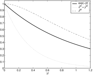
Figure 3: The effective channel $[x^{\mathrm{bf}}(t),y^{\mathrm{bf}}(t),z^{\mathrm{bf}}(t)]$ due to the bitflip code under the symmetric depolarizing channel. The respective fidelities of $X$, $Y$ and $Z$ eigenstates for correction performed at time $t$ are given by $\frac{1}{2}(1+x^{\mathrm{bf}}(t))$, $\frac{1}{2}(1+y^{\mathrm{bf}}(t))$, and $\frac{1}{2}(1+z^{\mathrm{bf}}(t))$.

More generally, for any $0<x,z<1$ we have $\frac{3}{2}z-\frac{1}{2}z^{3}>z$ and $x^{3}<x$, so for any physical channel in this regime the bitflip code always suppresses decoherence of $\langle Z\rangle$ and increases decoherence of $\langle X\rangle$. Decoherence of $\langle Y\rangle$ is suppressed when $x>\sqrt{\frac{2}{3}}$ and $0<y<\sqrt{3x^{2}-2}$, and increased for all other positive values of $x$ and $y$. We may therefore conclude that under a general Pauli channel the bitflip code increases the fidelity of some transmitted states at the expense of others, and thus the bitflip code is outperformed by storing the logical qubit in a single physical bit.

However, as the bitflip code is designed to only protect against physical bitflip ($X$) errors, it should not be expected to perform well in the presence of arbitrary Pauli errors. If we consider physical channels with only $X$ errors, we find that the bitflip code suppresses decoherence of all encoded states. More precisely, suppose that the physical qubits are evolving via a Pauli channel (36) with only $X$ errors, i.e. $p_{Y}=p_{Z}=0$. Then $[x,y,z]=[1,1-2p_{X},1-2p_{X}]$, and $\Omega^{\mathrm{bf}}([x,y,z])=[1,1-\frac{3}{2}p_{X}^{2}+\frac{1}{2}p_{X}^{3},1-\frac{3}{2}p_{X}^{2}+\frac{1}{2}p_{X}^{3}]$. Thus we have reproduced the usual result of a leading-order analysis: the bitflip code suppresses decoherence due to $X$ errors to order $p_{X}^{2}$.

Now consider the three-qubit phaseflip code Nielsen and Chuang (2000), with encoding $|\pm\rangle\mapsto|\pm\pm\pm\rangle$ for $|\pm\rangle=\frac{1}{\sqrt{2}}(|0\rangle+|1\rangle)$. This code is completely analogous to the bitflip code, detecting and correcting single phaseflip ($Z$) errors instead of single bitflip ($X$) errors. The phaseflip code’s coding map $\Omega^{\mathrm{pf}}$ is exactly the same as that of the bitflip code, with the role of $X$ and $Z$ interchanged:

$$\Omega^{\mathrm{pf}}([x,y,z])=\left[\tfrac{3}{2}x-\tfrac{1}{2}x^{3},\>\tfrac{3}{2}z^{2}y-\tfrac{1}{2}y^{3},\>z^{3}\right].$$ (39)

The concatenation phaseflip(bitflip) yields the Shor nine-bit code Shor (1995); Nielsen and Chuang (2000) with encoding $|\pm\rangle\mapsto\frac{1}{\sqrt{8}}(|000\rangle\pm|111\rangle)^{\otimes 3}$. Thus $\Omega^{\mathrm{Shor}}=\Omega^{\mathrm{pf}}\circ\Omega^{\mathrm{bf}}$. Evaluating this composition using the coding maps (38) and (39),

$$\Omega^{\mathrm{Shor}}([x,y,z]) = \Omega^{\mathrm{pf}}(\Omega^{\mathrm{bf}}([x,y,z]))$$ (40)

$$= [P(x),Q(x,y,z),R(z)]$$

where

$$\begin{array}[]{rcl}P(x)&=&\tfrac{3}{2}x^{3}-\tfrac{1}{2}x^{9}\\ Q(x,y,z)&=&\tfrac{3}{2}\left(\tfrac{3}{2}z-\tfrac{1}{2}z^{3}\right)^{2}\left(\tfrac{3}{2}x^{2}y-\tfrac{1}{2}y^{3}\right)\\ &&-\tfrac{1}{2}\left(\tfrac{3}{2}x^{2}y-\tfrac{1}{2}y^{3}\right)^{3}\\ R(z)&=&\left(\tfrac{3}{2}z-\tfrac{1}{2}z^{3}\right)^{3}.\end{array}$$ (41)

(The combinatoric analysis required to reproduce this result by counting bitflip and phaseflip errors would be quite tedious!)

To examine the Shor code acting on the symmetric depolarizing channel, let $[x^{\mathrm{Shor}}(t),y^{\mathrm{Shor}}(t),z^{\mathrm{Shor}}(t)]=\Omega^{\mathrm{Shor}}(\mathcal{N}^{\mathrm{dep}}_{t})$; the functions $x^{\mathrm{Shor}}$, $y^{\mathrm{Shor}}$ and $z^{\mathrm{Shor}}$ are plotted in Figure 4. We see that for short times (or equivalently, weak noise-strength $\gamma$), the Shor code suppresses decoherence of $\langle X\rangle$, $\langle Y\rangle$, and $\langle Z\rangle$. For long times, however, the code increases the decoherence of all three expectation values, and as $z^{\mathrm{Shor}}(t)>x^{\mathrm{Shor}}(t)>y^{\mathrm{Shor}}(t)$, in an intermediate regime the code suppresses the decoherence of some of the expectation values while increasing that of others. Thus to suppress the decoherence of an arbitrary logical state, correction needs to be performed at a time $t$ when $y^{\mathrm{Shor}}(t)>e^{-\gamma t}$.

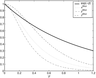
Figure 4: The effective channel $[x^{\mathrm{Shor}}(t),y^{\mathrm{Shor}}(t),z^{\mathrm{Shor}}(t)]$ due to the Shor code under the symmetric depolarizing channel.

Above we defined the phaseflip code by the encoding $|\pm\rangle\mapsto|\pm\pm\pm\rangle$; we could have also used the encoding given by $|0\rangle\mapsto|+++\rangle$, $|1\rangle\mapsto|---\rangle$. Call the code with this encoding phaseflip^′, with coding map $\Omega^{\mathrm{pf}^{\prime}}$. As this modification of the phaseflip code simply interchanges the encoded $X$- and $Z$-eigenstates, the new effective channel is simply that of the original phaseflip code with the effects of the channel on the $X$ and $Z$ components of $\vec{\rho}_{0}$ interchanged: $\Omega^{\mathrm{pf}^{\prime}}([x,y,z])=[z^{3},\frac{3}{2}z^{2}y-\frac{1}{2}y^{3},\frac{3}{2}x-\frac{1}{2}x^{3}]$ (compare to (39)). We could then use this version of the phaseflip code to define an alternative version of the Shor code with the encoding $|0\rangle\mapsto\frac{1}{\sqrt{8}}(|000\rangle+|111\rangle)^{\otimes 3}$, $|1\rangle\mapsto\frac{1}{\sqrt{8}}(|000\rangle-|111\rangle)^{\otimes 3}$. Call this code Shor^′, with corresponding coding map $\Omega^{\mathrm{Shor}^{\prime}}=\Omega^{\mathrm{pf}^{\prime}}\circ\Omega^{\mathrm{bf}}$. We find

$$\Omega^{\mathrm{Shor}^{\prime}}([x,y,z])=[R(z),Q(x,y,z),P(x)].$$ (42)

with the polynomials $P$, $Q$ and $R$ defined by (41). Comparing to (40), we see that again this modification of the Shor code simply interchanges the effect of the channel on $X$ and $Z$ components of $\vec{\rho}_{0}$. Assuming that the encoded logical states are randomly distributed (as opposed to always sending $Z$-eigenstates, for example), the choice of using the Shor code or the Shor^′ code is simply one of aesthetics: the effective channels are identical up to interchange of the decoherence of $\langle X\rangle$ and $\langle Z\rangle$. However, as we will see in the next section, this choice does have an impact when these codes are concatenated.

For comparison, we consider two other stabilizer codes of interest. The Steane code Nielsen and Chuang (2000); Steane (1996) is a seven-bit code designed to correct errors consisting either of a Pauli error ($X$, $Y$, or $Z$) on a single qubit of the codeword, or of an $X$ and a $Z$ error on separate qubits. We find

$$\Omega^{\mathrm{Steane}}([x,y,z])=[S(x),T(x,y,z),S(z)]$$ (43)

with

$$\begin{array}[]{rcl}S(x)&=&\tfrac{7}{4}x^{3}-\tfrac{3}{4}x^{7}\\ T(x,y,z)&=&\tfrac{7}{16}y^{3}+\tfrac{9}{16}y^{7}-\tfrac{21}{16}(x^{4}+z^{4})y^{3}+\tfrac{21}{8}x^{2}yz^{2}.\end{array}$$ (44)

Let $[x^{\mathrm{Steane}}(t),y^{\mathrm{Steane}}(t),z^{\mathrm{Steane}}(t)]=\Omega^{\mathrm{Steane}}(\mathcal{N}^{\mathrm{dep}}_{t})$; we find that the functions $x^{\mathrm{Steane}}$, $y^{\mathrm{Steane}}$ and $z^{\mathrm{Steane}}$ are qualitatively similar to the analogous functions of the Shor code. If they were plotted in Figure 4, these functions would be interspersed between the plotted curves: for all values of $t>0$, we have $z^{\mathrm{Shor}}>z^{\mathrm{Steane}}=x^{\mathrm{Steane}}>x^{\mathrm{Shor}}>y^{\mathrm{Steane}}>y^{\mathrm{Shor}}$. Though the Shor code more effectively suppresses decoherence for logical $Z$-eigenstates, the Steane code performs better in the worst case ($Y$-eigenstates), and thus outperforms the Shor code.

The Five-Bit code Nielsen and Chuang (2000); Laflamme et al. (1996); Bennett et al. (1996) corrects Pauli errors on a single qubit of the codeword. We find

$$\Omega^{\mathrm{Five}}([x,y,z])=[U(x,y,z),U(y,z,x),U(z,x,y)]$$ (45)

with

$$U(x,y,z)=\tfrac{5}{4}x(y^{2}+z^{2})-\tfrac{5}{4}xy^{2}z^{2}-\tfrac{1}{4}x^{5}.$$ (46)

Letting $[x^{\mathrm{Five}}(t),y^{\mathrm{Five}}(t),z^{\mathrm{Five}}(t)]=\Omega^{\mathrm{Five}}(\mathcal{N}^{\mathrm{dep}}_{t})$ yields $x^{\mathrm{Five}}=y^{\mathrm{Five}}=z^{\mathrm{Five}}$, as expected from the symmetries of the code and of the map $\Omega^{\mathrm{Five}}$. Thus the fidelity of a state through this channel is independent of the state. These functions also have qualitatively similar behavior to those plotted in Figure 4, and for $t>0$ we have $z^{\mathrm{Shor}}>z^{\mathrm{Five}}>z^{\mathrm{Steane}}>x^{\mathrm{Shor}}$. Thus the Five-Bit code outperforms both the Shor and Steane codes.

VII Exact Performance and Thresholds for Certain Concatenation Schemes

We now consider the effective channel due to families of concatenated codes under the symmetric depolarizing channel. First, consider the Shor code concatenated with itself $\ell$ times, denoted by Shor^ℓ. From section IV, we know that the coding map for this code is given by $\Omega^{(\mathrm{Shor}^{\ell})}=\Omega^{\mathrm{Shor}}\circ\ldots\circ\Omega^{\mathrm{Shor}}=(\Omega^{\mathrm{Shor}})^{\ell}$. As $\Omega^{\mathrm{Shor}}$ takes diagonal channels to diagonal channels , the effective channel due to Shor^ℓ is also diagonal. Let

$$[x_{\ell}(t),y_{\ell}(t),z_{\ell}(t)]=(\Omega^{\mathrm{Shor}})^{\ell}(\mathcal{N}^{\mathrm{dep}}_{t}),$$ (47)

which may be calculated using the polynomials of $\Omega^{\mathrm{Shor}}$ given in (41).

The functions $z_{\ell}(t)$ for $0\leq\ell\leq 4$ are plotted in Figure 5. We immediately observe that as $\ell\rightarrow\infty$ the functions $z_{\ell}(t)$ approach a step function. Denoting the step function’s time of discontinuity by $t_{Z}^{\star}$, we have $z_{\ell}(t)\rightarrow\theta(t_{Z}^{\star}-t)$ where

$$\theta(x)=\left\{\begin{array}[]{ccc}0&&x<0\\ 1&&x>0\end{array}\right..$$ (48)

For $t<t_{Z}^{\star}$, each layer of concatenation decreases the $\langle Z\rangle$ decoherence, yielding perfect preservation of the encoded $\langle Z\rangle$ information in the infinite concatenation limit. However, for $t>t_{Z}^{\star}$, the $\langle Z\rangle$ decoherence increases. Thus in the infinite concatenation limit, the code will perfectly protect $\langle Z\rangle$ of the logical qubit if correction is performed prior to $t_{Z}^{\star}$; if correction is performed after this time, all $\langle Z\rangle$ information is lost.

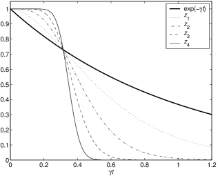
Figure 5: The functions $z_{\ell}$, where $[x_{\ell}(t),y_{\ell}(t),z_{\ell}(t)]$ is the effective channel for $\ell$ concatenations of the Shor code under the symmetric depolarizing channel.

Similarly, the functions $x_{\ell}(t)$ and $y_{\ell}(t)$ approach step function limits as $\ell\rightarrow\infty$; call the discontinuous times of these step functions $t_{X}^{\star}$ and $t_{Y}^{\star}$. To perfectly protect an arbitrary state in the infinite concatenation limit, correction must be performed prior to $t_{\mathrm{th}}=\min(t_{X}^{\star},t_{Y}^{\star},t_{Z}^{\star})$. We call $t_{\mathrm{th}}$ the storage threshold. (We use the term “storage threshold” to indicate that the threshold takes into account only noise in the register, rather than gate or measurement errors also considered in fault-tolerant settings.) We now show how the coding map $\Omega^{\mathrm{Shor}}$ may be used to find this threshold.

Observe in Figure 5 that the plots of $z_{\ell}(t)$ all intersect at a point $(\gamma t_{Z}^{\star},z^{\star})$. Writing $\Omega^{\mathrm{Shor}}$ in the form (40), we have $z_{\ell+1}(t)=R(z_{\ell}(t))$. The function $R(z)$ is plotted in Figure 6. We see that the map $z\mapsto R(z)$ has fixed points at $0$, $1$, and a point $z^{\star}\approx 0.7297$. (We find $z^{\star}$ by numerically solving $z=R(z)$ on the interval $(0,1)$.) Iterating the map pushes points in the interval $(0,z^{\star})$ toward $0$, and pushes points in the interval $(z^{\star},1)$ toward $1$. In the language of dynamical systems Devaney (1989), $0$ and $1$ are attracting fixed points, and $z^{\star}$ is a repelling fixed point. This behavior leads to the shape of the plots in Figure 5. We then invert $e^{-\gamma t_{Z}^{\star}}=z^{\star}$ to find $\gamma t_{Z}^{\star}=0.3151$. The function $P(x)$ has the same qualitative behavior on $(0,1)$ as $R(z)$, so we may similarly find $x^{\star}\approx 0.9003$ and $\gamma t_{X}^{\star}\approx 0.1050$.

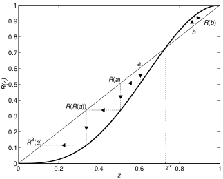
Figure 6: The function $R(z)$ (plotted as the thick curve). Observe that the map $z\mapsto R(z)$ has fixed points at 0, 1, and $z^{\star}$. The arrows depict the iteration of this map pushing points in the interval $(0,z^{\star})$ toward 0 and points in the interval $(z^{\star},1)$ toward 1.

We cannot use the same method to find $t_{Y}^{\star}$, as $y_{\ell+1}(t)$ is a function of $x_{\ell}(t)$, $y_{\ell}(t)$ and $z_{\ell}(t)$, not just of $y_{\ell}(t)$ alone. (This problem is evident from plots of the functions $y_{\ell}(t)$: though these functions approach a step function in the $\ell\rightarrow\infty$ limit, they do not all intersect at a point as the plots of $z_{\ell}(t)$ do.) However, we now argue that finding $t_{X}^{\star}$ and $t_{Z}^{\star}$ is sufficient to find $t_{Y}^{\star}$. For $t<t_{X}^{\star}$, $x_{\ell}(t)\rightarrow 1$ and $z_{\ell}(t)\rightarrow 1$. Using the complete positivity constraints (35), we find that if $[x,y,z]$ is a channel, $x=z=1$ implies $y=1$. Since the space of channels $[x,y,z]$ is closed and bounded (it consists of the boundary and interior of a tetrahedron in $\mathbb{R}^{3}$), $x_{\ell}(t)\rightarrow 1$ and $z_{\ell}(t)\rightarrow 1$ implies $y_{\ell}(t)\rightarrow 1$. Now for $t_{X}^{\star}<t<t_{Z}^{\star}$, $x_{\ell}(t)\rightarrow 0$ and $z_{\ell}(t)\rightarrow 1$. Using the complete positivity constraints (35), we find that if $[x,y,z]$ is a channel, $x=0$ and $z=1$ implies $y=0$. Thus we may conclude that for these values of $t$, $y_{\ell}(t)\rightarrow 0$. We now have $y_{\ell}(t)\rightarrow 1$ for $t<t_{X}^{\star}$, and $y_{\ell}(t)\rightarrow 0$ for $t>t_{X}^{\star}$, thus we conclude $t_{Y}^{\star}=t_{X}^{\star}$. More generally, if we know $t_{X}^{\star}$ and $t_{Z}^{\star}$, then $t_{Y}^{\star}$ is given by $\min(t_{X}^{\star},t_{Z}^{\star})$. We may therefore conclude that $\gamma t_{Y}^{\star}\approx 0.1050$, and so $\gamma t_{\mathrm{th}}\approx 0.1050$. (The value of $t_{Y}^{\star}$ could also be obtained from the dynamics of the polynomial maps $P$, $Q$ and $R$ without making reference to the complete positivity constraint, but the method presented here requires less argumentation.)

We may also phrase these thresholds in the language of finitely probable errors. Consider the symmetric Pauli channel given by (36) with $p_{X}=p_{Y}=p_{Z}=\frac{p}{3}$. This channel subjects a qubit to a random Pauli error with probability $p$, and is described by $\mathcal{N}^{\mathrm{Pauli}}(p)=[1-\frac{4}{3}p,1-\frac{4}{3}p,1-\frac{4}{3}p]$. Observe that the symmetric Pauli channel and the symmetric depolarizing channel are related by $\mathcal{N}^{\mathrm{Pauli}}(\frac{3}{4}(1-e^{-\gamma t}))=\mathcal{N}^{\mathrm{dep}}_{t}$. Thus in the infinite concatenation limit with $\mathcal{N}^{\mathrm{Pauli}}(p)$ acting on each register qubit, the $\langle\sigma\rangle$ of the logical qubit will be perfectly protected if $p<p^{\star}_{\sigma}=\frac{3}{4}(1-e^{-\gamma t^{\star}_{\sigma}})$. Define the threshold probability $p_{\mathrm{th}}=\min\{p^{\star}_{X},p^{\star}_{Y},p^{\star}_{Z}\}$; for $p<p_{\mathrm{th}}$, all encoded qubits are perfectly protected in the infinite concatenation limit. Values for $\gamma t^{\star}_{\sigma}$ and $p_{\mathrm{th}}$ appear in Table 1.

Code	Shor		Shor′		Steane	Five-Bit
$\sigma$	$X,Y$	$Z$	$X,Y$	$Z$	$X,Y,Z$	$X,Y,Z$
$\gamma t_{\sigma}^{\star}$	0.1050	0.3151	0.1618	0.2150	0.1383	0.2027
$p_{\mathrm{th}}$	0.0748		0.1121		0.0969	0.1376

Table 1: Code storage threshold results. (See text for discussion.)

We now use similar methods to derive thresholds for the Shor^′, Steane, and Five-Bit codes presented in the previous section. First, consider the Shor^′ code. Let $[x^{\prime}_{\ell}(t),y^{\prime}_{\ell}(t),z^{\prime}_{\ell}(t)]=(\Omega^{\mathrm{Shor}^{\prime}})^{\ell}(\mathcal{N}^{\mathrm{dep}}_{t})$. The $y^{\prime}_{\ell}(t)$ approach a step function as $\ell\rightarrow\infty$, but $x^{\prime}_{\ell}(t)$ and $z^{\prime}_{\ell}(t)$ approach a limit cycle of period 2: we find that $x^{\prime}_{2\ell}$ and $z^{\prime}_{2\ell+1}$ both approach $\theta(t_{1}^{\star}-t)$ for some value of $t_{1}^{\star}$, while $x^{\prime}_{2\ell+1}$ and $z^{\prime}_{2\ell}$ approach $\theta(t_{2}^{\star}-t)$ for some distinct value of $t_{2}^{\star}$. From the form of $\Omega^{\mathrm{Shor}^{\prime}}$ given in (42), we see that $x^{\prime}_{\ell+1}(t)$ is a function of $z^{\prime}_{\ell}(t)$, and $z^{\prime}_{\ell+1}(t)$ a function of $x^{\prime}_{\ell}(t)$, so it is not so surprising that the sequence $z^{\prime}_{0},x^{\prime}_{1},z^{\prime}_{2},x^{\prime}_{3},\ldots$ converges and the sequence $x^{\prime}_{0},z^{\prime}_{1},x^{\prime}_{2},z^{\prime}_{3},\ldots$ converges. To find the threshold, we simply consider the sequence of channels $[x^{\prime}_{2\ell},y^{\prime}_{2\ell},z^{\prime}_{2\ell}]$, generated by the map $(\Omega^{\mathrm{Shor}^{\prime}})^{2}$. From (42) we see that $x^{\prime}_{2(\ell+1)}=R(P(x^{\prime}_{2\ell}))$ and $z^{\prime}_{2(\ell+1)}=P(R(z^{\prime}_{2\ell}))$. Thus to find the values $t_{X}^{\star}$, $t_{Y}^{\star}$ and $t_{Z}^{\star}$, we find the fixed points of the maps $x\mapsto R(P(x))$ and $z\mapsto P(R(z))$, and proceed as with the Shor code. As shown in Table 1, we find that, compared to the Shor code, the Shor^′ code has greater values for $t_{X}^{\star}$ and $t_{Y}^{\star}$, and a lesser value for $t_{Z}^{\star}$. As the threshold $t_{\mathrm{th}}$ is given by the minimum of these three values, the Shor^′ code outperforms the Shor code in the infinite concatenation limit.

The map $\Omega^{\mathrm{Steane}}$, given by (43), has the same form as the Shor code map (40), and therefore we can use the same methods to find the Steane code thresholds. The map $\Omega^{\mathrm{Five}}$, given by (45), has a different form. However, as $\mathcal{N}^{\mathrm{dep}}_{t}$ has the symmetric form $[x,x,x]$ and $\Omega^{\mathrm{Five}}$ preserves this symmetry by taking $[x,x,x]$ to $[U(x,x,x),U(x,x,x),U(x,x,x)]$, we may find $t_{X}^{\star}=t_{Y}^{\star}=t_{Z}^{\star}$ simply by finding the fixed point of $x\mapsto U(x,x,x)$. Results are summarized in Table 1. We find that the Five-Bit code has the largest threshold, and therefore the best performance in the infinite concatenation limit. It is interesting to note that the Shor^′ code outperforms the Steane code in the infinite concatenation limit, even though the opposite is true for only one layer of each code.

We conclude our discussion of the thresholds by comparing the exact values of $p_{\mathrm{th}}$ to those calculated with traditional leading-order techniques (e.g. in Nielsen and Chuang (2000)). First consider the Five-Bit code. Under the symmetric Pauli channel $\mathcal{N}^{\mathrm{Pauli}}(p)$, a physical qubit is unmodified with probability $1-p$. The Five-Bit code perfectly protects its encoded information if no more than one of the five physical qubits are subjected to a Pauli error. Under $\mathcal{N}^{\mathrm{Pauli}}(p)$, the probability of no errors on any physical qubit is $(1-p)^{5}$, and the probability of exactly one error is $5p(1-p)^{4}$. We then assume that all greater-weight errors are uncorrectable, and find that the probability of a correctable error is $(1-p)^{5}+5p(1-p)^{4}=1-10p^{2}+O(p^{3})$. The threshold value $p_{\mathrm{th}}$ is the value of $p$ at which the single physical qubit and the encoded information have the same probability of error. Thus to estimate the threshold we solve $1-10p^{2}=1-p$, yielding $p_{\mathrm{th}}=\frac{1}{10}$. Thus the leading-order calculation underestimates the actual threshold (0.1376) by $27\%$. (The assumption that all errors of greater weight are uncorrectable assures that the approximation underestimates, rather than overestimates, the threshold.) The Steane code corrects all weight-one errors, and weight-two errors consisting of an $X$ on one bit and a $Z$ on another bit. A similar calculation finds the probability of a correctable error to be $1-\frac{49}{3}p^{2}+O(p^{3})$, yielding $p_{\mathrm{th}}\approx 0.0612$, a $37\%$ underestimate. The Shor code corrects all weight-one errors, and weight-two errors such that any $X$ and $Y$ operators occur in different blocks, and any $Y$ and $Z$ errors occur in the same block. The probability of a correctable error is found to be $1-16p^{2}+O(p^{3})$, yielding $p_{\mathrm{th}}=0.0625$, a $16\%$ underestimate. The analysis is exactly the same for the Shor^′ code, yet the Shor^′ code has a very different threshold; in this case, the leading-order result underestimates the threshold by $44\%$.

VIII Conclusion

We have shown how a code’s performance for a given error model can be described by the effective channel for the encoded information. The methods presented for calculating the effective channel have allowed us to find the performance of several codes of interest under single-bit Pauli channels, and further have allowed us to find thresholds describing these codes’ asymptotic limits of concatenation under the symmetric depolarizing channel. Though we chose to restrict our attention to diagonal channels, these methods can be applied to any uncorrelated error model (e.g. the amplitude-damping channel Nielsen and Chuang (2000), which is non-diagonal), and will substantially simplify the exact analysis of code performance in these more general settings.

We believe that this effective channel description of code performance may be useful in other contexts as well. For example, this work could be extended to take account of encoding and decoding circuit errors, thereby providing a method for calculating exact fault-tolerant thresholds. Also, by providing a comprehensive method for describing the performance of a quantum code without reference to a particular error model (e.g. bitflip and phaseflip errors) perhaps these methods will allow us to address open questions such as the optimal code for a given error model, and the quantum channel capacity.

Appendix A Stabilizer Codes and Diagonal Channels

In this appendix we consider the effective channel $\mathcal{G}=\Omega^{C}(\mathcal{N}^{(1)})$ when $\mathcal{N}^{(1)}$ is diagonal and $C$ is a stabilizer code. We show that $\mathcal{G}$ is also diagonal, and show how the stabilizer formalism facilitates its calculation. The reader unfamiliar with stabilizer codes is directed to Nielsen and Chuang (2000) for an introduction, and to Gottesman (1997) for a more complete discussion.

Since $\mathcal{N}^{(1)}$ is diagonal, the terms $N^{(1)}_{\nu_{i}\mu_{i}}$ in the expression for the effective channel (25) vanish for $\nu_{i}\neq\mu_{i}$. Thus we have

$$\mathcal{G}_{\sigma\sigma^{\prime}}=\sum_{\{\mu_{i}\}}\left(\beta_{\{\mu_{i}\}}^{\sigma}\alpha_{\{\mu_{i}\}}^{\sigma^{\prime}}\prod_{i=1}^{N}\mathcal{N}^{(1)}_{{\mu_{i}}{\mu_{i}}}\right),$$ (49)

dramatically simplifying the calculation of $\mathcal{G}$. The coefficients $\alpha_{\{\mu_{i}\}}^{\sigma^{\prime}}$ and $\beta_{\{\mu_{i}\}}^{\sigma}$ are defined in terms of the $E_{\sigma^{\prime}}$ and $D_{\sigma}$ operators in (20) and (21); to calculate these operators we now consider the code $C$ in more detail.

Let $C$ be a stabilizer code given by stabilizer $S=\{S_{k}\}\subset\pm\{I,X,Y,Z\}^{\otimes N}$, storing one qubit in an $N$-qubit register. The stabilizer $S$ defines the codespace, and the logical operators $\bar{I},\bar{X},\bar{Y},\bar{Z}\subset\pm\{I,X,Y,Z\}^{\otimes N}$ determine the particular basis of codewords $|\overline{0}\rangle$, $|\overline{1}\rangle$. Recall that the $E_{\sigma^{\prime}}$ operators act as $\frac{1}{2}\sigma^{\prime}$ on the codespace and vanish elsewhere. It can be shown that $P_{C}=\frac{1}{|S|}\sum_{k}S_{k}$ acts as a projector onto the codespace, and by definition the logical operators $\bar{\sigma}^{\prime}$ act as $\sigma^{\prime}$ on the codespace. Thus

$$E_{\sigma^{\prime}}=\tfrac{1}{2}P_{C}\bar{\sigma}^{\prime}=\tfrac{1}{2|S|}\sum_{k}S_{k}\bar{\sigma}^{\prime}$$ (50)

will act as $\frac{1}{2}\sigma^{\prime}$ on the codespace and vanish elsewhere.

As an example, consider the bitflip code introduced in section II.1. The bitflip code may be specified as a stabilizer code, with $S=\{III,ZZI,IZZ,ZIZ\}$, $\bar{I}=III$, $\bar{X}=XXX$, $\bar{Y}=-YYY$, $\bar{Z}=ZZZ$. The above expression reproduces the expressions for the $E_{\sigma^{\prime}}$ presented in (22). Without the stabilizer formalism, deriving (22) is an exercise in expanding projectors in a basis of Pauli operators; with this method the computation is very simple.

We now construct the $D_{\sigma}$ operators for the stabilizer code. As in section II.1, let $\{P_{j}\}$ be the projectors describing the syndrome measurement. For a stabilizer code, the recovery operators $R_{j}$ are each chosen to be a Pauli operator taking the space projected by $P_{j}$ back to the codespace. Consider the expression for $D_{\sigma}$ given by (16); substituting in the expression (50) for $E_{\sigma}$, we have

$$D_{\sigma}=\tfrac{1}{|S|}\sum_{k,j}R_{j}^{\dagger}S_{k}\bar{\sigma}R_{j}.$$ (51)

Now because $R_{j}$, $S_{k}$ and $\bar{\sigma}$ are all Pauli operators, they either commute or anti-commute. For two Pauli operators $V$ and $W$, let $\eta(V,W)=\pm 1$ for $VW=\pm WV$. Commuting the $R_{j}$ to the left in the above expression and noting that $R_{j}^{\dagger}R_{j}=1$,

$$\begin{array}[]{rcl}D_{\sigma}&=&\tfrac{1}{|S|}\sum_{k,j}\eta(S_{k},R_{j})\eta(R_{j},\bar{\sigma})S_{k}\bar{\sigma}\\ &=&\tfrac{1}{|S|}\sum_{k}f_{k\sigma}S_{k}\bar{\sigma}\end{array}$$ (52)

with $f_{k\sigma}=\sum_{j}\eta(S_{k},R_{j})\eta(R_{j},\bar{\sigma})$. Again, as an example consider the stabilizer definition of the bitflip code. The recovery operators are $III$, $XII$, $IXI$, and $IXI$. Evaluating the above expression for $D_{\sigma}$ yields the previous result of (23).

Using the expressions (50) and (52) for the $E_{\sigma^{\prime}}$ and $D_{\sigma}$ operators in the stabilizer formalism, we we will now find the coefficients $\alpha_{\{\mu_{i}\}}^{\sigma^{\prime}}$ and $\beta_{\{\nu_{i}\}}^{\sigma}$ as defined in (20) and (21). Since $S_{k}\bar{\sigma}$ is a Pauli operator, the sums (50) and (52) are expansions of these operators $E_{\sigma^{\prime}}$ and $D_{\sigma}$ in the Pauli basis; if we were to write down these sums explicitly for a given stabilizer code, the coefficients $\alpha$ and $\beta$ could be read off immediately, e.g. from (22) and (23).

This approach may be formalized as follows. First, note that $S_{k}$ and $\bar{\sigma}$ are both Hermitian Pauli operators, and they commute; therefore their product is also a Hermitian Pauli operator, i.e. $S_{k}\bar{\sigma}\in\pm\{I,X,Y,Z\}^{\otimes N}$. For any operator $V=\pm\mu_{1}\otimes\ldots\otimes\mu_{N}$ with $\mu_{i}\in\{I,X,Y,Z\}$, let $\phi(V)=\mu_{1}\otimes\ldots\otimes\mu_{N}$, and let $a(V)\in\{0,1\}$ such that $V=(-1)^{a(V)}\phi(V)$. Then, using $|S|=2^{N-1}$, we may re-write (50) and (52) as

$$E_{\sigma^{\prime}} = \sum_{k}(-1)^{a(S_{k}\bar{\sigma}^{\prime})}\tfrac{1}{2^{N}}\phi(S_{k}\bar{\sigma}^{\prime})$$ (53)

$$D_{\sigma} = \sum_{k}(-1)^{a(S_{k}\bar{\sigma})}\tfrac{1}{|S|}f_{k\sigma}\phi(S_{k}\bar{\sigma}).$$ (54)

Comparing (53) with the definition of $\alpha^{\sigma^{\prime}}_{\{\mu_{i}\}}$ in (20), we see that each term of the sum over $k$ contributes to a single coefficient $\alpha^{\sigma^{\prime}}_{\phi(S_{k}\bar{\sigma}^{\prime})}$, as $\frac{1}{2^{N}}\phi(S_{k}\bar{\sigma}^{\prime})$ is of the form $(\frac{1}{2}\mu_{1}\otimes\ldots\otimes\frac{1}{2}\mu_{N})$. Similarly, each term in (54) contributes to a single coefficient $\beta^{\sigma}_{\phi(S_{k}\bar{\sigma})}$. Lemma 2 of Appendix B shows that $\phi(S_{k}\bar{\sigma})\neq\phi(S_{k^{\prime}}\bar{\sigma})$ unless $k=k^{\prime}$ and $\sigma=\sigma^{\prime}$. Thus each term in (53) contributes to a distinct coefficient $\alpha^{\sigma^{\prime}}_{\phi(S_{k}\bar{\sigma}^{\prime})}$, and each term in (54) contributes to a distinct coefficient $\beta^{\sigma}_{\phi(S_{k}\bar{\sigma})}$. We may therefore simply read off the coefficients from (53) and (54), yielding

$$\alpha^{\sigma^{\prime}}_{\phi(S_{k}\bar{\sigma}^{\prime})} = (-1)^{a(S_{k}\bar{\sigma}^{\prime})}$$ (55)

$$\beta^{\sigma}_{\phi(S_{k}\bar{\sigma})} = (-1)^{a(S_{k}\bar{\sigma})}\tfrac{1}{|S|}f_{k\sigma},$$ (56)

and all other $\alpha^{\sigma^{\prime}}_{\{\mu_{i}\}}$ and $\beta^{\sigma}_{\{\mu_{i}\}}$ vanishing.

We now evaluate $\mathcal{G}=\Omega^{C}(\mathcal{N}^{(1)})$ where $\mathcal{N}^{(1)}=[x,y,z]$ using (49). The only non-vanishing terms $\beta_{\{\mu_{i}\}}^{\sigma}$ occur when $\mu_{1}\otimes\ldots\otimes\mu_{N}=\phi(S_{k}\bar{\sigma})$ for some $k$ and $\sigma$, and the only the only non-vanishing terms $\alpha_{\{\mu_{i}\}}^{\sigma^{\prime}}$ occur when $\mu_{1}\otimes\ldots\otimes\mu_{N}=\phi(S_{k}\bar{\sigma}^{\prime})$ for some $k$ and $\sigma^{\prime}$. Thus the coefficients $\beta_{\{\mu_{i}\}}^{\sigma}\alpha_{\{\mu_{i}\}}^{\sigma^{\prime}}$ of (49) will vanish unless $\mu_{1}\otimes\ldots\otimes\mu_{N}=\phi(S_{k}\bar{\sigma})=\phi(S_{k^{\prime}}\bar{\sigma}^{\prime})$ for some $k$ and $k^{\prime}$. As proved in Lemma 2 of Appendix B, this cannot happen when $\sigma\neq\sigma^{\prime}$. Thus all the matrix elements $\mathcal{G}_{\sigma\sigma^{\prime}}$ vanish when $\sigma\neq\sigma^{\prime}$, i.e. $\mathcal{G}$ is diagonal.

Having demonstrated that the coding map $\Omega^{C}$ of a stabilizer code $C$ takes diagonal channels to diagonal channels, and because $\mathcal{G}_{II}=1$ from trace preservation, we need only compute $\mathcal{G}_{XX}$, $\mathcal{G}_{YY}$, and $\mathcal{G}_{ZZ}$ using (49) to find $\mathcal{G}=\Omega^{C}([x,y,z])$. These computations can be performed using the methods of section III, but we conclude this section by expressing these elements using the stabilizer formalism, which may be computationally advantageous.

Consider the diagonal terms $\mathcal{G}_{\sigma\sigma}$ given by (49). We need only sum over the non-vanishing coefficients $\alpha$ and $\beta$, which are given by (55) and (56). Substituting in these expressions yields

$$\mathcal{G}_{\sigma\sigma}=\sum_{k}\left(\frac{1}{|S|}f_{k\sigma}\prod_{i=1}^{N}\mathcal{N}^{(1)}_{\phi_{i}(S_{k}\bar{\sigma})\phi_{i}(S_{k}\bar{\sigma})}\right)$$ (57)

where $\phi_{i}(V)$ denotes $\mu_{i}$ for $\phi(V)=\mu_{1}\otimes\ldots\otimes\mu_{N}$. Now as $\mathcal{N}^{(1)}=[x,y,z]$, the product of the matrix elements of $\mathcal{N}^{(1)}$ in the previous expression is simply a product of $x$’s, $y$’s and $z$’s; each factor appears as many times as (respectively) $X$, $Y$ and $Z$ appear in $\phi(S_{k}\bar{\sigma})$. Letting $w_{\sigma}(p)$ denote the $\sigma$-weight of a Pauli operator $p$, e.g. $w_{X}(XYX)=2$, we have

$$\mathcal{G}_{\sigma\sigma^{\prime}}=\delta_{\sigma\sigma^{\prime}}\frac{1}{|S|}\sum_{k}f_{k\sigma}x^{w_{X}(S_{k}\bar{\sigma})}y^{w_{Y}(S_{k}\bar{\sigma})}z^{w_{Z}(S_{k}\bar{\sigma})}.$$ (58)

Appendix B

This appendix contains lemmas deferred from previous sections.

Lemma 1: The decoding operation $\mathcal{D}$ given by (4) is a quantum operation.

Proof: From (4) we have

$$\mathcal{D}[\rho]=\sum_{j}B^{\dagger}A_{j}\rho A_{j}^{\dagger}B.$$ (59)

To prove that $\mathcal{D}$ is a quantum operation, we must show

$$\sum_{j}(A_{j}^{\dagger}B)(B^{\dagger}A_{j})=\mathbf{1}$$ (60)

where $\mathbf{1}$ is the identity on the register space. As we assumed that $\mathcal{R}$ maps all states into the codespace, we can choose the operators $A_{j}$ to only have range on the codespace. With such a choice, $A_{j}^{\dagger}A_{j}=A_{j}^{\dagger}(|\overline{0}\rangle\langle\overline{0}|+|\overline{1}\rangle\langle\overline{1}|)A_{j}=A_{j}^{\dagger}BB^{\dagger}A_{j}$. We therefore have

$$\sum_{j}(A_{j}^{\dagger}B)(B^{\dagger}A_{j})=\sum_{j}A_{j}^{\dagger}A_{j}.$$ (61)

From (3) we have $\sum_{j}A_{j}^{\dagger}A_{j}=\mathbf{1}$, and so $\mathcal{D}$ is a quantum operation. $\blacksquare$

Lemma 2: For a stabilizer code with stabilizer $\{S_{k}\}$ and logical operators $\{\bar{\sigma}\}$, and $\phi$ defined in Appendix A, $\phi(S_{k}\bar{\sigma})\neq\phi(S_{k^{\prime}}\bar{\sigma}^{\prime})$ unless $k=k^{\prime}$ and $\sigma=\sigma^{\prime}$.

Proof: Suppose we have $\phi(S_{k}\bar{\sigma})=\phi(S_{k^{\prime}}\bar{\sigma}^{\prime})$; then $S_{k}\bar{\sigma}=\pm S_{k^{\prime}}\bar{\sigma}^{\prime}$. As the stabilizers $S_{k}$ and $S_{k^{\prime}}$ act trivially on the codespace, $S_{k}\bar{\sigma}$ and $\pm S_{k^{\prime}}\bar{\sigma}^{\prime}$ act respectively as $\sigma$ and $\pm\sigma^{\prime}$ on the codespace. Thus we must have $\sigma=\pm\sigma^{\prime}$, which requires $\sigma=\sigma^{\prime}$ and the $\pm$ sign be positive. We now have $S_{k}\bar{\sigma}=S_{k^{\prime}}\bar{\sigma}$; right-multiplying by $\bar{\sigma}$ yields $S_{k}=S_{k^{\prime}}$, and thus $k=k^{\prime}$. $\blacksquare$

References

- Shor (1995) P. W. Shor, “Scheme for Reducing Decoherence in Quantum Computer Memory”, Phys. Rev. A 52, 2493 (1995).
- Steane (1996) A. M. Steane, “Error Correcting Codes in Quantum Theory”, Phys. Rev. Lett. 77, 793 (1996).
- Nielsen and Chuang (2000) M. A. Nielsen and I. L. Chuang, Quantum Computation and Quantum Information (Cambridge University Press, 2000), and references therein; J. Preskill, Lecture Notes, http://theory.caltech.edu/preskill/ph219 (1998).
- Preskill (1997) J. Preskill, “Fault-tolerant Quantum Computation”, eprint quant-ph/9712048 (1997), and references therein.
- Knill and Laflamme (1996) E. Knill and R. Laflamme, “Concatenated Quantum Codes”, eprint quant-ph/9698012 (1996).
- Knill and Laflamme (1997) E. Knill and R. Laflamme, “Theory of Quantum Error-Correcting Codes”, Phys. Rev. A 55, 900 (1997).
- Kraus (1983) K. Kraus, States, Effect, and Operations (Springer-Verlag, 1983).
- Ruskai et al. (2001) M. B. Ruskai, S. Szarek, et al., “An Analysis of Completely-Positive Trace-Preserving Maps on ”, eprint quant-ph/0101003 (2001).
- Lidar et al. (2001) D. A. Lidar, D. Bacon, et al., “Decoherence-Free Subspaces for Multiple-Qubit Errors I: Characterization”, Phys. Rev. A 63, 022306 (2001).
- Devaney (1989) R. L. Devaney, An Introduction to Chaotic Dynamical Systems (Addison-Wesley, 1989).
- King and Ruskai (2001) C. King and M. B. Ruskai, “Minimal Entropy of States Emerging from Noisy Quantum Channels”, IEEE Trans. Info. Theory 47, 192 (2001), eprint quant-ph/9911079.
- Gottesman (1997) D. Gottesman, “Stabilizer Codes and Quantum Error Correction”, Ph.D. thesis, Caltech (1997), eprint quant-ph/9705052.
- Laflamme et al. (1996) R. Laflamme, C. Miqel, et al., “Perfect Quantum Error Correcting Code”, Phys. Rev. Lett. 77, 198 (1996).
- Bennett et al. (1996) C. H. Bennett, D. P. DiVincenzo, et al., “Mixed-State Entanglement and Quantum Error Correction”, Phys. Rev. A 54, 3824 (1996).