Abstract

We investigate the capacity of three symmetric quantum states in three real dimensions to carry classical information. Several such capacities have already been defined, depending on what operations are allowed in the sending and receiving protocols. These include the $C_{1,1}$ capacity, which is the capacity achievable if separate measurements must be used for each of the received states, and the $C_{1,\infty}$ capacity, which is the capacity achievable if joint measurements are allowed on the tensor product of all the received states. We discover a new classical information capacity of quantum channels, the adaptive capacity $C_{1,A}$, which lies strictly between the $C_{1,1}$ and the $C_{1,\infty}$ capacities. The adaptive capacity allows what is known as the LOCC (local operations and classical communication) model of quantum operations for decoding the channel outputs. This model requires each of the signals to be measured by a separate apparatus, but allows the quantum states of these signals to be measured in stages, with the first stage partially reducing their quantum states, and where measurements in subsequent stages may depend on the results of a classical computation taking as input the outcomes of the first round of measurements. We also show that even in three dimensions, with the information carried by an ensemble containing three pure states, achieving the $C_{1,1}$ capacity may require a POVM with six outcomes.

1 Introduction

For classical channels, Shannon’s theorem [16] gives the information-carrying capacity of a channel. When one tries to generalize this to quantum channels, there are several ways to formulate the problem which have given rise to several different capacities. In this paper, we consider the capacity of quantum channels to carry classical information, with various restrictions on how the channel may be used. Several such capacities have already been defined for quantum channels. In particular, the $C_{1,1}$ capacity, where only tensor product inputs and tensor product measurements are allowed [3, 10, 11, 12], and the $C_{1,\infty}$ capacity, where tensor product inputs and joint measurements are allowed [8, 15, 7], have both been studied extensively. We will be investigating these capacities in connection with a specific example; namely, we analyze how these capacities behave on a symmetric set of three quantum states in three dimensions which we call the lifted trine states. A quantum channel of the type that Holevo [7] classifies as c-q (classical-quantum) can be constructed from these states by allowing the sender to choose one of these three pure states, which is then conveyed to the receiver. This channel is simple enough that we can analyze the behavior of various capacities for it, but it is also complicated enough to exhibit interesting behaviors which have not been observed before. In particular, we define a new, natural, classical capacity for a quantum channel, the $C_{1,A}$ capacity, which we also call the adaptive one-shot capacity, and show that it is strictly between the $C_{1,1}$ capacity (also called the one-shot quantum capacity) and the $C_{1,\infty}$ capacity (also called the Holevo capacity).

The three states we consider, the lifted trine states, are obtained by starting with the two-dimensional quantum trine states, $(1,0)$, $(-1/2,\sqrt{3}/2)$, $(-1/2,-\sqrt{3}/2)$ introduced by Holevo [6] and later studied by Peres and Wootters [13]. We add a third dimension to the Hilbert space of the trine states, and lift all of the trine states out the plane into this dimension by an angle of $\arcsin\sqrt{\alpha}$, so the states become $(\sqrt{1-\alpha},0,\sqrt{\alpha})$, and so forth. We will be dealing with small $\alpha$ (roughly, $\alpha<0.1$), so that they are close to being planar. This is one of the interesting regimes. When the trine states are lifted further out of the plane, they behave in less interesting ways until they are close to being vertical; then they start being interesting again, but we will not investigate this second regime.

To put this channel into the formulation of completely positive trace-preserving operators, we let the sender start with a quantum state in a three-dimensional input state space, measure this state using a von Neumann measurement with three outcomes, and send one of the lifted trines $T_{0}$, $T_{1}$ or $T_{2}$, depending on the outcome of this measurement. This process turns any quantum state into a probability distribution over $T_{0}$, $T_{1}$ and $T_{2}$.

The first section of the paper deals with the accessible information for the lifted trine states when the probability of all three states is equal. The accessible information of an ensemble is the maximum mutual information obtainable between the input states of the ensemble and the outcomes of a POVM (positive operator valued measure) measurement on these states. The substance of this section has already appeared, in [17]. Combined with Appendix C, this shows that the number of projectors required to achieve the $C_{1,1}$ capacity for the ensemble of lifted trines can be as large as 6, the maximum possible by the real version of Davies’ theorem. The second section deals with the $C_{1,1}$ channel capacity (or the one-shot capacity), which is the maximum of the accessible information over all probability distributions on the trine states. This has often been called the $C_{1}$ capacity because it is the classical capacity obtained when you are only allowed to process (i.e., encode/measure) one signal at a time. We call it $C_{1,1}$ to emphasize that you are only allowed to input tensor product states (the first 1), and only allowed to make quantum measurements on one signal at a time (the second 1). The third section deals with the new capacity $C_{1,A}$, the “adaptive one-shot capacity.” This is the capacity for sending classical information attainable if you are allowed to send codewords composed of tensor products of lifted trine states, are not allowed to make joint measurements involving more than one trine state, but are allowed to make a measurement on one signal which only partially reduces the quantum state, use the outcome of this measurement to determine which measurement to make on a different signal, return to refine the measurement on the first signal, and so forth. In Section 5, we give an upper bound on the $C_{1,1}$ capacity of the lifted trine states, letting us show that for the lifted trine states with sufficiently small $\alpha$, this adaptive capacity is strictly larger than the $C_{1,1}$ channel capacity. In section 6, we show and that for two pure non-orthogonal states, $C_{1,A}$ is equal to $C_{1,1}$, and thus strictly less than the Holevo capacity $C_{1,\infty}$. These two results show show that $C_{1,A}$ is different from previously defined capacities for quantum channels. To obtain a capacity larger than $C_{1,1}$, it is necessary to make measurements that only partially reduce the state of some of the signals, and then later return to refine the measurement on these signals depending on the results of intervening measurement. In Section 7, we show if you use “sequential measurement”, i.e., only measure one signal at a time, and never return to a previously measured signal, it is impossible to achieve a capacity larger than $C_{1,1}$.

We take the lifted trine states to be:

$$T_{0}(\alpha) = (\sqrt{1-\alpha},0,\sqrt{\alpha})$$

$$T_{1}(\alpha) = (-{\textstyle{\frac{1}{2}}}\sqrt{1-\alpha},{\textstyle{\frac{\sqrt{3}}{2}}}\sqrt{1-\alpha},\sqrt{\alpha})$$ (1)

$$T_{2}(\alpha) = (-{\textstyle{\frac{1}{2}}}\sqrt{1-\alpha},-{\textstyle{\frac{\sqrt{3}}{2}}}\sqrt{1-\alpha},\sqrt{\alpha})$$

When it is clear what $\alpha$ is, we may drop it from the notation and use $T_{0}$, $T_{1}$, or $T_{2}$.

2 The Accessible Information

In this section, we find the accessible information for the ensemble of lifted trine states, given equal probabilities. This is defined as the maximal mutual information between the trine states (with probabilities $\frac{1}{3}$ each) and the elements of a POVM measuring these states. Because the trine states are vectors over the reals, it follows from the generalization of Davies’ theorem to real states (see, e.g., [14]) that there is an optimal POVM with at most six elements, all the components of which are real. The lifted trine states are three-fold symmetric, so by symmetrizing we can assume that the optimal POVM is three-fold symmetric (possibly at the cost of introducing extra POVM elements). Also, the optimal POVM can be taken to have one-dimensional elements $E$, so the elements can be described as vectors $\left|\,v_{i}\right\rangle$ where $E_{i}=\left|\,v_{i}\right\rangle\left\langle v_{i}\,\right|$. This means that there is an optimal POVM whose vectors come in triples of the form: $\sqrt{p}P_{0}(\phi,\theta)$, $\sqrt{p}P_{1}(\phi,\theta)$, $\sqrt{p}P_{2}(\phi,\theta)$, where $p$ is a scalar probability and

$$P_{0}(\phi,\theta) = (\cos\phi\cos\theta,\cos\phi\sin\theta,\sin\phi)$$

$$P_{1}(\phi,\theta) = (\cos\phi\cos(\theta+2\pi/3),\cos\phi\sin(\theta+2\pi/3),\sin\phi)$$ (2)

$$P_{2}(\phi,\theta) = (\cos\phi\cos(\theta-2\pi/3),\cos\phi\sin(\theta-2\pi/3),\sin\phi).$$

The optimal POVM may have several such triples, which we label $\sqrt{p_{1}}\,P_{b}(\phi_{1},\theta_{1})$, $\sqrt{p_{2}}\,P_{b}(\phi_{2},\theta_{2})$, $\ldots$, $\sqrt{p_{m}}\,P_{b}(\phi_{m},\theta_{m})$. It is easily seen that the conditions for this set of vectors to be a POVM are that

$$\sum_{i=1}^{m}p_{i}\sin^{2}(\phi_{i})=1/3{\mathrm{\quad and\quad}}\sum_{i=1}^{m}p_{i}=1.$$ (3)

One way to compute the accessible information $I_{A}$ is to break the formula for accessible information into pieces so as to keep track of the amount of information contributed to it by each triple. That is, $I_{A}$ will be the weighted average (weighted by $p_{i}$) of the contribution $I(\phi,\theta)$ from each $(\phi,\theta)$. To see this, recall that $I_{A}$ is the mutual information between the input and the output, and that this can be expressed as the entropy of the input less the entropy of the input given the output, $H(X_{\mathrm{in}})-H(X_{\mathrm{in}}|X_{\mathrm{out}})$. The term $H(X_{\mathrm{in}}|X_{\mathrm{out}})$ naturally decomposes into terms corresponding to the various POVM outcomes, and there are several ways of assigning the entropy of the input $H(X_{\mathrm{in}})$ to these POVM elements in order to complete this decomposition. This is how I first arrived at the formula for $I_{A}$. I briefly sketch this analysis, and then go into detail in a second analysis. This second analysis is superior in that it explains the form of the answer obtained, but it is not clear how one could discover the second analysis without first knowing the result.

For each $\phi$, and each $\alpha$, there is a $\theta$ that optimizes $I(\phi,\theta)$. This $\theta$ starts out at $\pi/6$ for $\phi=0$, decreases until it hits 0 at some value of $\phi$ (which depends on $\alpha$), and stays at $0$ until $\phi$ reaches its maximum value of $\pi/2$. For a fixed $\alpha$, by finding (numerically) the optimal value of $\theta$ for each $\phi$ and using it to obtain the contribution to $I_{A}$ attributable to that $\phi$, we get a curve giving the optimal contribution to $I_{A}$ for each $\phi$. If this curve is plotted, with the $x$-value being $\sin^{2}\phi$ and the $y$-value being the contribution to $I_{A}$, an optimal POVM can be obtained by finding the set of points on this curve whose average $x$-value is $1/3$ (from Eq. 3), and whose average $y$-value is as large as possible. A convexity argument shows that we only need at most two points from the curve to obtain this optimum; we will need one or two points depending on whether the relevant part of the curve is concave or convex. For small $\alpha$, it can be seen numerically that the relevant piece of the curve is convex, and we need two $\phi$’s to achieve the maximum. One of the $(\phi,\theta)$ pairs is $(0,\pi/6)$, and the other is $(\phi_{\alpha},0)$ for some $\phi_{\alpha}>\arcsin(1/\sqrt{3})$. The formula for this $\phi_{\alpha}$ will be derived later. Each of these $\phi$’s corresponds to a triple of POVM elements, giving six elements for the optimal POVM.

The analysis in the remainder of this section gives a different way of describing this six-outcome POVM. This analysis unifies the measurements for different $\alpha$, and also introduces some of the methods that will appear again in Section 4. Consider the following measurement protocol. For small $\alpha$ ($\alpha<\gamma_{1}$ for some constant $\gamma_{1}$), we first take the trine $T_{b}(\alpha)$ and make a partial measurement which either projects it onto the $x,y$ plane or lifts it further out of this plane so that it becomes the trine $T_{b}(\gamma_{1})$. (Here $\gamma_{1}$ is independent of $\alpha$.) If the measurement projects the trine into the $x,y$ plane, we make a second measurement using the POVM having outcome vectors $\sqrt{2/3}(0,1)$ and $\sqrt{2/3}(\pm\sqrt{3}/2,-1/2)$. This is the optimal POVM for trines in the $x,y$-plane. If the measurement lifts the trine further out of the $x,y$ plane, we use the von Neumann measurement that projects onto the basis consisting of $(\sqrt{2/3},0,\sqrt{1/3})$, $(-\sqrt{1/6},\pm\sqrt{1/2},\sqrt{1/3})$. If $\alpha$ is larger than $\gamma_{1}$ (but smaller than $8/9$), we skip the first partial measurement, and just use the above von Neumann measurement. Here, $\gamma_{1}$ is obtained by numerically solving a fairly complicated equation; we suspect that no closed form expression for it exists. The value of $\gamma_{1}$ is 0.061367, which is $\sin^{2}\phi$ for $\phi\approx 0.25033$ radians ($14.343^{\circ}$).

We now give more details on this decomposition of the POVM into a two-step process. We first apply a partial measurement which does not extract all of the quantum information, i.e., it leaves a quantum residual state that is not completely determined by the measurement outcome. Formally, we apply one of a set of matrices $A_{i}$ satisfying $\sum_{i}A_{i}^{\dagger}A_{i}=I$. If we start with a pure state $\left|\,v\right\rangle$, we observe the $i$’th outcome with probability $\left\langle v\,\right|A_{i}^{\dagger}A_{i}\left|\,v\right\rangle$, and in this case the state $\left|\,v\right\rangle$ is taken to the state $A_{i}\left|\,v\right\rangle$. We choose as the $A_{i}$’s the matrices $\sqrt{p_{i}}\,M(\phi_{i})$ where

$$M(\phi)=\left(\begin{array}[]{ccc}\sqrt{\frac{3}{2}}\cos\phi&0&0\\ 0&\sqrt{\frac{3}{2}}\cos\phi&0\\ 0&0&\sqrt{3}\sin\phi\end{array}\right)$$ (4)

The $\sqrt{p_{i}}\,M(\phi_{i})$ form a valid partial measurement if and only if

$$\sum_{i}p_{i}\sin^{2}(\phi_{i})=1/3\mathrm{\ \ \ and\ \ }\sum_{i}p_{i}=1.$$

By first applying the above $\sqrt{p_{i}}\,M(\phi_{i})$, and then applying the von Neumann measurement with the three basis vectors

$$V_{0}(\theta) = \textstyle\Big{(}\sqrt{\frac{2}{3}}\cos\theta,\sqrt{\frac{2}{3}}\sin\theta,\frac{1}{\sqrt{3}}\Big{)}$$

$$V_{1}(\theta) = \textstyle\Big{(}\sqrt{\frac{2}{3}}\cos(\theta+2\pi/3),\sqrt{\frac{2}{3}}\sin(\theta+2\pi/3),\frac{1}{\sqrt{3}}\Big{)}$$ (5)

$$V_{2}(\theta) = \textstyle\Big{(}\sqrt{\frac{2}{3}}\cos(\theta-2\pi/3),\sqrt{\frac{2}{3}}\sin(\theta-2\pi/3),\frac{1}{\sqrt{3}}\Big{)}$$

we obtain the POVM given by the vectors $\sqrt{p_{i}}\,P_{b}(\theta_{i},\phi_{i})$ of Eq. (2); checking this is simply a matter of verifying that $V_{b}(\theta)M(\phi)=P_{b}(\theta,\phi)$. Now, after applying $\sqrt{p_{i}}\,M(\phi_{i})$ to the trine $T_{0}(\alpha)$, we get the vector

$$\big{(}\sqrt{3/2}\sqrt{1-\alpha}\sqrt{p_{i}}\cos\phi_{i},0,\sqrt{3}\sqrt{\alpha}\sqrt{p_{i}}\sin\phi_{i}\big{)}.$$ (6)

This is just the state $\sqrt{p_{i}^{\prime}}\,T_{0}(\alpha_{i}^{\prime})$ where $T_{0}(\alpha_{i}^{\prime})$ is the trine state with

$$\alpha_{i}^{\prime}=\frac{\alpha\sin^{2}\phi_{i}}{\alpha\sin^{2}\phi_{i}+\frac{1}{2}(1-\alpha)\cos^{2}\phi_{i}},$$ (7)

and where

$$p_{i}^{\prime}=3p_{i}\left[\alpha\sin^{2}\phi+{\textstyle{\frac{1}{2}}}(1-\alpha)\cos^{2}\phi\right]$$ (8)

is the probability that we observe this trine state, given that we started with $T_{0}(\alpha)$. Similar formulae hold for the trine states $T_{1}$ and $T_{2}$. We compute that

$$\sum_{i}p_{i}^{\prime}\alpha_{i}^{\prime}=\sum_{i}3p_{i}\alpha\sin^{2}(\phi_{i})=\alpha.$$ (9)

The first stage of this process, the partial measurement which applies the matrices $\sqrt{p_{i}}\,M(\phi_{i})$, reveals no information about which of $T_{0}$, $T_{1}$, $T_{2}$ we started with. Thus, by the chain rule for classical Shannon information [2], the accessible information obtained by our two-stage measurement is just the weighted average (the weights being $p^{\prime}_{i}$) of the maximum over $\theta$ of the Shannon mutual information $I_{\alpha_{i}^{\prime}}(\theta)$ between the outcome of the von Neumann measurement $V(\theta)$ and the trine $T(\alpha_{i}^{\prime})$. By convexity, it suffices to use only two values of $\alpha_{i}^{\prime}$ to obtain this maximum. In fact, the optimum is obtained using either one or two values of $\alpha_{i}^{\prime}$ depending on whether the function

$$I_{\alpha^{\prime}}=\max_{\theta}I_{\alpha^{\prime}}(\theta)$$

is concave or convex over the appropriate region. In the remainder of this section, we give the results of computing (numerically) the values of this function $I_{\alpha^{\prime}}$. For small enough $\alpha$ it is convex, so that we need two values of $\alpha^{\prime}$, corresponding to a POVM with six outcomes.

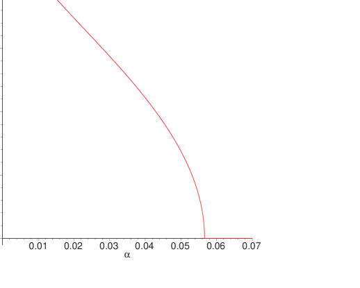
Figure 1: The value of $\theta$ maximizing $I_{\alpha}$ for $\alpha$ between $0$ and $0.07$. This function starts at $\pi/6$ at $\alpha=0$, decreases until it hits $0$ at $\alpha=0.056651$ and stays at $0$ for larger $\alpha$.

We need to calculate the Shannon capacity of the classical channel whose input is one of the three trine states $T(\alpha^{\prime})$, and whose output is determined by the von Neumann measurement $V(\theta)$. Because of the symmetry, we can calculate this using only the first projector $V_{0}$. The Shannon mutual information between the input and the output is $H(X_{\mathrm{in}})-H(X_{\mathrm{in}}|X_{\mathrm{out}})$, which is

$$I_{\alpha^{\prime}}=\log_{2}3+\sum_{b=0}^{2}\left|\langle V_{0}(\theta)|T_{b}(\alpha^{\prime})\rangle\right|^{2}\log_{2}\left|\langle V_{0}(\theta)|T_{b}(\alpha^{\prime})\rangle\right|^{2}.$$ (10)

The $\theta$ giving the maximum $I_{\alpha}^{\prime}$ is $\pi/6$ for $\alpha^{\prime}=0$, decreases continuously to 0 at $\alpha^{\prime}=0.056651$, and remains 0 for larger $\alpha^{\prime}$. (See Fig. 1.) This value $0.056651$ corresponds to an angle of 0.24032 radians ($13.769^{\circ}$). This $\theta$ was determined by using the computer package Maple to numerically find the point at which $dI_{\alpha}(\theta)/d\theta=0$.

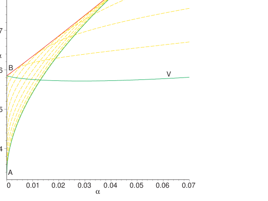
Figure 2: This plot shows $I_{\alpha}(\theta)$ for $0\leq\alpha\leq 0.07$ and various $\theta$. This is the mutual information between the lifted trines at an angle of $\arcsin\sqrt{\alpha}$ to the $x$-$y$ plane, and a von Neumann measurement rotated with respect to these trines by an angle $\theta$. The green curve AZ is $I_{\alpha}(0)$ and the green curve BV is $I_{\alpha}(\pi/6)$. The $\theta=0$ curve is optimal for $\alpha>0.056651$, and $\theta=\pi/6$ is optimal for $\alpha=0$. The dashed yellow curves show $I_{\alpha}(\theta)$ for $\theta$ at intervals of $3^{\circ}$ between $0^{\circ}$ and $30^{\circ}$ ($\pi/6$ radians). Finally, the red curve BZ shows $I_{\alpha}(\theta_{\rm opt})$ for those $\alpha$ where neither $0$ nor $\pi/6$ is the optimal $\theta$. The function $\theta_{\mathrm{opt}}$ is given in Figure 1. It is hard to see from this plot, but the red curve BZ is slightly convex, i.e., its second derivative is positive. This is clearer in Fig. 3.

By plugging the optimum $\theta$ into the formula for $I_{\alpha^{\prime}}$, we obtain the optimum von Neumann measurement of the form $V$ above. We believe this is also the optimal generic von Neumann measurement, but have not proved this. The maximum of $I_{\alpha^{\prime}}(\theta)$ over $\theta$, and curves that show the behavior of $I_{\alpha^{\prime}}(\theta)$ for constant $\theta$, are plotted in Fig. 2. We can now observe that the leftmost piece of the curve is convex, and thus that for small $\alpha$ the best POVM will have six projectors, corresponding to two values of $\alpha^{\prime}$. For trine states with $0<\alpha<0.061367$, the two values of $\alpha^{\prime}$ giving the maximum accessible information are $0$ and $0.061367$; we call this second value $\gamma_{1}$. The trine states $T(\gamma_{1})$ make an angle of 0.25033 radians ($14.343^{\circ}$) with the $x$-$y$ plane.

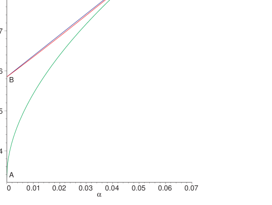
Figure 3: This graph contains three curves. As in Fig. 2, the green curve AZ is $I_{\alpha}(0)$ and the red curve BZ is the maximum over $\theta$ of $I_{\alpha}(\theta)$ for $\alpha<0.056651$ (for larger $\alpha$, this maximum is the green curve). The blue line BZ is straight; it is the convex envelope of the red and green curves and lies slightly above the red curve BZ. This blue line is a linear interpolation between $\alpha=0$ and $\alpha=0.061367$ and corresponds to a POVM having six elements. It gives the accessible information for the lifted trine states $T(\alpha)$ when $0\leq\alpha\leq 0.061367$. The difference between the blue and red curves is maximum at $\alpha=0.024831$, when this difference reaches $0.0038282$.

We can now invert the formula for $\alpha^{\prime}$ (Eq. 7) to obtain a formula for $\sin^{2}\phi$, and substitute the value of $\alpha^{\prime}=\gamma_{1}$ back into the formula to obtain the optimal POVM. We find

$$\sin^{2}(\phi_{\alpha}) = \frac{1-\alpha}{1+\alpha\left(\frac{2-3\gamma_{1}}{\gamma_{1}}\right)}$$ (11)

$$\approx \frac{1-\alpha}{1+29.591\alpha}$$

where $\gamma_{1}\approx 0.061367$ as above. Thus, the elements in the optimal POVM we have found for the trines $T(\alpha)$, when $\alpha<\gamma_{1}$, are the six vectors $P_{b}(\phi_{\alpha},0)$ and $P_{b}(0,\pi/6)$, where $\phi_{\alpha}$ is given by Eq. 11 and $b=0,1,2$. Fig. 3 plots the accessible information given by this six-outcome POVM, and compares it to the accessible information obtained by the best known von Neumann measurement.

We also prove there are no other POVM’s which attain the same accessible information. The argument above shows that any optimal POVM must contain only projectors chosen from these six vectors: only those two values of $\alpha^{\prime}$ can appear in the measurement giving maximum capacity, and for each of these values of $\alpha^{\prime}$ there are only three projectors in $V(\theta)$ which can maximize $I_{\alpha^{\prime}}$ for these $\alpha^{\prime}$. It is easy to check that there is only one set of probabilities $p_{i}$ which make the above six vectors into a POVM, and that none of these probabilities are 0 for $0<\alpha<\gamma_{1}$. Thus, for the lifted trine states with $0<\alpha<\gamma_{1}$, there is only one POVM maximizing accessible information, and it contains six elements, the maximum possible for real states by a generalization of Davies’ theorem [14].

3 The $\mathbf{C_{1,1}}$ Capacity

In this section, we discuss the $C_{1,1}$ capacity (or one-shot capacity) of the lifted trine states. This is the maximum of the accessible information over all probability distributions of the lifted trine states. Because the trine states are real vectors, it follows from a version of Davies’ theorem that there is an optimal POVM with at most six elements, all the components of which are real. Since the lifted trine states are three-fold symmetric, one might expect that the solution maximizing $C_{1,1}$ capacity is also three-fold symmetric. However, unlike accessible information, for $C_{1,1}$ capacity a symmetric problem does not mean that the optimal probabilities and the optimal measurement can be made symmetric. Indeed, for the planar trine states, it is known that they cannot. The optimal $C_{1,1}$ capacity for the planar trine states $T(0)$ is obtained by assigning probability $1/2$ to two of the three states and not using the third one at all. (See Appendix A.) This gives a channel capacity of $1-H(1/2-\sqrt{3}/4)=0.64542$ bits, where $H(x)=-x\log_{2}x-(1-x)\log_{2}(1-x)$ is the binary Shannon entropy. As discussed in the previous section, the accessible information when all three trine states have equal probability is $\log_{2}3-1=0.58496$ bits.

In this section, we first discuss the best measurement we have found to date. We believe this is likely to be the optimal measurement, but do not have a proof of this. Later, we will discuss what we can actually prove; namely, that as $\alpha$ approaches 0 (i.e., for nearly planar trine states), the actual $C_{1,1}$ capacity becomes exponentially close to the value given by our conjectured optimal measurement. We postpone this proof to Section 5 so that in Section 4 we can complete our presentation of the various channel capacities of the lifted trine states by giving an adaptive protocol that improves on our conjectured $C_{1,1}$ capacity. Together with the bounds in Section 5, this lets us prove that the adaptive capacity $C_{1,A}$ is strictly larger than $C_{1,1}$.

Our starting point is the $C_{1,1}$ capacity for planar trines. The optimum probability distribution uses just two of the three trines. For two pure states, $\left|\,v_{1}\right\rangle$ and $\left|\,v_{2}\right\rangle$, the optimum measurement for $C_{1,1}$ is known. Let the states have an angle $\theta$ between them, so that $\big{|}\langle v_{1}|v_{2}\rangle\big{|}^{2}=\cos^{2}\theta$. We can then take the two states to be $v_{1}=(\cos\frac{\theta}{2},\sin\frac{\theta}{2})$ and $v_{2}=(\cos\frac{\theta}{2},-\sin\frac{\theta}{2})$. The optimal measurement is the von Neumann measurement with projectors $P{\pm}=(1/\sqrt{2},\pm 1/\sqrt{2})$. This measurement induces a classical binary symmetric channel with error probability

$$\langle P_{+}|v_{2}\rangle^{2} = \cos^{2}(\theta/2+\pi/4)$$

$$= \frac{1-\sin\theta}{2}.$$

and the $C_{1,1}$ capacity is thus $1-H(\frac{1}{2}-\frac{1}{2}\sin\theta)$. Thus, for the planar trines, the $C_{1,1}$ capacity is $1-H(1/2-\sqrt{3}/4)=0.64542$. To obtain our best guess for the $C_{1,1}$ capacity of the lifted trines with $\alpha$ small, we will give three successively better guesses at the optimal probability distribution and measurement. For small $\alpha$, we know of nothing better than the third guess, which we conjecture to be optimal when $\alpha<0.018073$. John Smolin has tried searching for solutions using a hill-climbing optimization program, and failed to find any better measurement for $C_{1,1}$, although the program did converge to the best known value a significant fraction of the time [18].

For the trines $T(0)$, the optimum probability distribution is $(\frac{1}{2},\frac{1}{2},0)$. Our first guess is to continue to use the same probability distribution for $\alpha>0$. For the trines $T(\alpha)$, this probability distribution, $(\frac{1}{2},\frac{1}{2},0)$, the optimum measurement is a von Neumann measurement with projectors

$$Q_{0}(\beta) = \ \left(\sqrt{\beta},0,\sqrt{1-\beta}\,\right)$$

$$Q_{1}(\beta) = \frac{1}{\sqrt{2}}\left(-\sqrt{1-\beta},1,\sqrt{\beta}\,\right)$$

$$Q_{2}(\beta) = \frac{1}{\sqrt{2}}\left(-\sqrt{1-\beta},-1,\sqrt{\beta}\,\right)$$ (12)

where $\beta=4\alpha/(3\alpha+1)$. The $C_{1,1}$ capacity in this case is $1-H(p)$ where $p=\frac{1}{2}(3\alpha-1)^{2}/(3\alpha+1)$. This function is plotted in Fig. 6. We call this the two-trine capacity.

,

Figure 4: The classical channel induced by the measurement $Q(4\alpha/(3\alpha+1))$ on the lifted trines $T(\alpha)$. The inputs, from top to bottom, correspond to $T_{1}$, $T_{2}$, and $T_{0}$; the outputs correspond to $Q_{1}$, $Q_{2}$ and $Q_{0}$. The transition probabilities are given above, where $\delta=\langle Q_{0}|T_{0}\rangle^{2}$ and $q=\langle Q_{1}|T_{2}\rangle^{2}=\langle Q_{2}|T_{1}\rangle^{2}$.

The second guess comes from using the same measurement, $Q(\beta)$, as the first guess, but varying the probabilities of the three trine states so as to maximize the $C_{1,1}$ capacity obtained using this measurement. To do this, we need to consider the classical channel shown in Fig. 4. Because of the symmetry of this channel, the optimal probability distribution is guaranteed to give equal probabilities to trines $T_{1}$ and $T_{2}$. Remarkably, this channel has a closed form for the probability $p$ for the third trine which maximizes the mutual information. Expressing the mutual information as $H(X_{\mathrm{out}})-H(X_{\mathrm{out}}|X_{\mathrm{in}})$, we find that this simplifies to

$$(1-p)(1-H(q))+H(p\delta)-pH(\delta)$$ (13)

where $\delta=\langle Q_{0}|T_{0}\rangle^{2}$ and $q=\langle Q_{2}|T_{1}\rangle^{2}=\langle Q_{1}|T_{2}\rangle^{2}$. Taking the derivative of this function with respect to $p$, setting it to 0, and moving the terms with $p$ in them to the left side of the equality gives

$$\delta\left[\log_{2}(1-p\delta)-\log_{2}(p)\right]=1-H(q)-(1-\delta)\log_{2}(1-\delta).$$ (14)

Dividing by $\delta$ and exponentiating both sides gives

$$\frac{1-\delta p}{p}=2^{\textstyle\,\frac{1}{\delta}\left({1-H(q)-(1-\delta)\log_{2}(1-\delta)}\right)}$$ (15)

which has the solution

$$p=\frac{1}{\delta+\exp\left(\frac{\log 2}{\delta}[1-H(q)-(1-\delta)\log_{2}(1-\delta)]\right)}.$$ (16)

Using this value of $p$, and the measurement of Eq. 12 with $\beta=4\alpha/(3\alpha+1)$, we obtain a curve that is plotted in Fig. 6. Note that as $\alpha$ goes to 0, $\delta$ goes to 0 and the exponential on the right side goes to $2^{[1-H(q)]/\delta}$, so $p$ becomes exponentially small. It follows that this function differs from the two-trine capacity by an exponentially small amount as $\alpha$ approaches $0$. Note also that no matter how small $\delta$ is, the above value of $p$ is non-zero, so even though the two-trine capacity is exponentially close to the above capacity, it is not equal.

For our third guess, we refine the above solution slightly. It turns out that the $\beta$ used to determine the measurement $Q(\beta)$ is no longer optimal after we have given a non-zero probability to the third trine state. What we do is vary both $p$ and $\beta$ to find the optimal measurement for a given $\alpha$. This leads to the classical channel shown in Fig. 5. Here,

1

Figure 5: The classical channel induced by the von Neumann measurement $Q(\beta)$ on the lifted trines $T(\alpha)$. The inputs correspond (top to bottom) to $T_{1}$, $T_{2}$ and $T_{0}$; the outputs correspond (top to bottom) to $Q_{1}$, $Q_{2}$ and $Q_{0}$.

$q$ and $\delta$ take the same values as above, and $\epsilon=\langle Q_{0}|T_{1}\rangle^{2}=\langle Q_{0}|T_{2}\rangle^{2}$. As we did for the case with $\epsilon=0$, we can write down the channel capacity, differentiate with respect to $p$, and solve the resulting equation. In this case, the solution turns out to be

$$p=\frac{1-\epsilon-\epsilon 2^{Z}}{(\delta-\epsilon)(1+2^{Z})}$$ (17)

where

$$Z=\frac{1-\epsilon-H(q;\epsilon;1-q-\epsilon)+H(\delta)}{\delta-\epsilon}.$$ (18)

Here

$$H(p_{1};p_{2};\cdots;p_{k})=\sum_{j=1}^{k}-p_{j}\log_{2}p_{j}$$

is the Shannon entropy of the probability distribution $\{p_{1},p_{2},\cdots,p_{k}\}$. We have numerically found the optimum $\beta$ for the measurement $Q(\beta)$, and used this result to obtain the $C_{1,1}$ capacity achieved by optimizing over both $p$ and $Q(\beta)$. This capacity function is shown in Fig. 6. This capacity, and the capacities obtained using various specific values of $\beta$ in $Q(\beta)$ are shown in Fig. 7. For $\alpha\geq 0.040491$, the optimum $\beta$ is $\frac{2}{3}$; note that the measurement $Q(\frac{2}{3})$ is the same as the measurement $V(0)$ introduced in Section 2, Eq. 5. The measurement $Q(\beta)$ appears to give the $C_{1,1}$ capacity for $\alpha\leq 0.018073$ [and for $\alpha\geq 0.061367$, where the optimum measurement is $Q(\frac{2}{3})$].

Now, suppose that in the above expression for $p$ [Eqs. (17) and (18)], $\epsilon$ and $\delta$ are both approaching $0$, while $q$ is bounded away from $\frac{1}{2}$. If $\delta>\epsilon$, then $2^{Z}$ is exponentially large in $1/(\delta-\epsilon)$, and the equation either gives a negative $p$ (in which case the optimum value of $p$ is actually $0$) or $p$ is exponentially small. If $\epsilon>\delta$, and both $\epsilon$ and $\delta$ are sufficiently small, then $2^{Z}$ is exponentially small in $1/(\epsilon-\delta)$ and the value of $p$ in the above equation is negative, so that the optimum value of $p$ is $0$. There are solutions to the above equation which have $\epsilon>\delta$ and positive $p$, but this is not the case when $\epsilon$ is sufficiently close to $0$.

It follows from the above argument that, as $\alpha$ goes to $0$, the optimum probability $p$ for the third trine state goes to $0$ exponentially fast in $1/\delta$, and so the $C_{1,1}$ capacity obtained from this measurement grows exponentially close to that for the two-trine capacity, since the two probability distributions differ by an exponentially small amount.

We have now described our conjectured $C_{1,1}$ for the lifted trine states, and the measurements and probability distributions that achieve it. In the next section, we will show that there is an adaptive protocol which achieves a capacity $C_{1,A}$ considerably better than our conjectured $C_{1,1}$ capacity. When $\alpha$ is close to $0$, it is better by an amount linear in $\alpha$. To rigorously prove that it is better, we need to find an upper bound on the capacity $C_{1,1}$ which is less than $C_{1,A}$. We already noted that, as $\alpha$ approaches $0$, all three of our guesses for $C_{1,1}$ become exponentially close. In Section 5 of this paper we prove that the true $C_{1,1}$ capacity must become exponentially close to these guesses.

Because these three guesses for $C_{1,1}$ become exponentially close near $\alpha=0$, they all have the same derivative with respect to $\alpha$ at $\alpha=0$. Our first guess, which used only two of the three trines, is simple enough that we can compute this derivative analytically, and we find that its value is

$$\frac{\sqrt{3}}{2}\log_{2}\left(2+\sqrt{3}\right)=1.64542{\hbox{\ bits.}}$$

This contrasts with our best adaptive protocol, which has the same capacity at $\alpha=0$, but which between $\alpha=0$ and $\alpha=0.087247$ has slope 4.42238 bits (see Fig. 10). Thus, for small enough $\alpha$, the adaptive capacity $C_{1,A}$ is strictly larger than $C_{1,1}$.

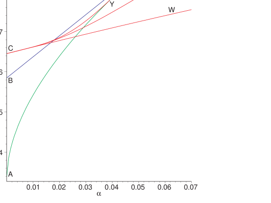
Figure 6: This graph contains five curves. The blue line BZ and the green curve AYZ are the same as in Fig. 3. The maximum of these two curves is the accessible information for the lifted trine states $T(\alpha)$ with equal probabilities for all three states. The maximum of all five curves is the conjectured $C_{1,1}$ capacity. The three red curves with left endpoint C are the three successively better guesses described in the text for the $C_{1,1}$ capacity. The lower red curve CW is the $C_{1,1}$ capacity for just two of the lifted trine states. The middle red curve CX is the capacity obtained using the same measurement $Q(4\alpha/(3\alpha+1))$ that gives the lower red curve CW, but with the probabilities of the three trine states optimized. Finally, the top red curve CY is the $C_{1,1}$ capacity obtained by optimizing both the probabilities and the measurement, but only over the limited class of measurements $Q(b)$. These three red curves become exponentially close to each other as $\alpha$ approaches 0.

,

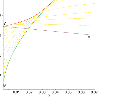
Figure 7: This figure shows the Shannon capacity obtained using various measurements on the trine states $T(\alpha)$, while optimizing the input probability distribution on the trines. The green curve AYZ is the same as in the previous figures. It is obtained using the von Neumann measurement $Q(2/3)$, which is also the measurement $V(0)$. The violet curve CV is obtained using the measurement $Q(0)$, which is optimal for the planar trines ($\alpha=0$). The dashed yellow curves are the capacities obtained by the measurement $Q(\sin^{2}\theta)$ where $\theta$ is taken at intervals of $5^{\circ}$ from $5^{\circ}$ to $50^{\circ}$. The violet curve CV corresponds to $\theta=0^{\circ}$ and the green curve AYZ to $\theta=54.736^{\circ}$. Finally, the red curve CY is the upper envelope of the dashed yellow curves; shows the capacity obtained by choosing the measurement $Q(\beta)$ with optimal $\beta$ for each $\alpha<0.040491$. For larger $\alpha$, this optimum is at $\beta=2/3$, and is given by the green curve YZ.

4 The Adaptive Capacity $\mathbf{C}_{1,A}$

As can be seen from Figure 6, the $C_{1,1}$ capacity is not concave in $\alpha$. That is, there are two values of $\alpha$ such that the average of their $C_{1,1}$ capacities is larger than the $C_{1,1}$ capacity of their average. This is analogous to the situation we found while studying the accessible information for the probability distribution $(\frac{1}{3},\frac{1}{3},\frac{1}{3})$, where the curve giving the information attainable by von Neumann measurements was also not concave. In that case, we were able to obtain the convex hull of this curve by using a POVM to linearly interpolate between the two von Neumann measurements. Remarkably, we show that for the lifted trines example, the relationship between $C_{1,1}$ capacity and $C_{1,A}$ capacity is similar: protocols using adaptive measurement can attain the convex hull of the $C_{1,1}$ capacity with respect to $\alpha$.

We now introduce the adaptive measurement model leading to the $C_{1,A}$ capacity. If we assume that each of the signals that Bob receives is held by a separate party, this is the same as the LOCC model used in [9, 1] where several parties share a quantum state and are allowed to use local quantum operations and classical communication between the parties. In our model, Alice sends Bob a tensor product codeword using the channel many times. We call the output from a single use of the channel a signal. Bob is not allowed to make joint quantum measurements on more than one signal, but he is allowed to make measurements sequentially on different signals. He is further allowed to use the classical outcomes of his measurements to determine which signal to measure next, and to determine which measurement to make on that signal. In particular, he is allowed to make a measurement which only partially reduces the quantum state of one signal, make intervening measurements on other signals, and return to make a further measurement on the reduced state of the original signal (which measurement may depend on the outcomes of intervening measurements). The information rate for a given encoding and measurement strategy is the mutual information between Alice’s codewords and Bob’s measurement outcomes, divided by the number of signals (channel uses) in the codeword. The adaptive one-shot capacity $C_{1,A}$ is defined to be the supremum of this information rate over all encodings and all measurement strategies that use quantum operations local to the separate signals (and classical computation to coordinate them). As we will show in Section 7, to exceed $C_{1,1}$ it is crucial to be able to refine a measurement made on a given signal after making intervening measurements on other signals.

In our adaptive protocol for lifted trines, we use two rounds of measurements. We first make one measurement on each of the signals received; this measurement only partially reduces the quantum state of some of the signals. We then make a second measurement (on some of the signals) which depends on the outcomes of the first round of measurements.

A precursor to this type of adaptive strategy appeared in an influential paper of Peres and Wootters [13] which was a source of inspiration for this paper. In their paper, Peres and Wootters studied strategies of adaptive measurement on the tensor product of two trine states, in which joint measurements on both copies were not allowed. They showed that for a specific encoding of block length 2, adaptive strategies could extract strictly more information than sequential strategies, but not as much as was extractable through joint measurements. However, the adaptive strategies they considered extracted less information than the $C_{1,1}$ capacity of the trine states, and so could have been improved on by using a different encoding and a sequential strategy. We show that for some values of $\alpha$, $C_{1,A}$ is strictly greater than $C_{1,1}$ for the lifted trines $T(\alpha)$, where these capacities are defined using arbitrarily large block lengths and arbitrary encodings. It is open whether $C_{1,1}=C_{1,A}$ for the planar trine states.

Before we describe our measurement strategy, we will describe the codewords we use for information transmission. The reason we choose these codewords will not become clear until after we have given the strategy. Alice will send one of these codewords to Bob, who with high probability will be able to deduce which codeword was sent from the outcomes of his measurements. These codewords are constructed using a two-stage scheme, corresponding to the two rounds of our measurement protocol. Effectively, we are applying Shannon’s classical channel coding theorem twice.

To construct a codeword, we take two error correcting codes each of block length $n$ and add them letterwise (mod 3). The first code is over a trinary alphabet (which we take to be $\{0,1,2\})$; it contains $2^{\tau_{1}n-o(n)}$ codewords, and is a good classical error-correcting code for a classical channel we describe later. The second code contains $2^{\tau_{2}n-o(n)}$ codewords, is over the binary alphabet $\{0,1\}$, and is a good classical error-correcting code for a different classical channel. Such classical error-correcting codes can be constructed by taking the appropriate number of random codewords; for the proof that our decoding strategy works, we will assume that the codes were indeed constructed this way. To obtain our code, we simply add these two codes bit-wise (mod 3). For example, if a codeword in the first (trinary) code is 0212 and a codeword in the second (binary) code is 1110, the codeword obtained by adding them bitwise is 1022. This new code contains $2^{(\tau_{1}+\tau_{2})n-o(n)}$ codewords (since we choose the two codes randomly, and we make sure that $\tau_{1}+\tau_{2}<\log_{2}3$).

To show how our construction works, we first consider the following measurement strategy. This is not the best protocol we have found, but it provides a good illustration of how our protocols work. This uses the two-level codeword scheme described above. In this protocol, the first measurement we make uses a POVM which contains four elements. One of them is a scalar times the matrix

$$\Pi_{xy}=\left(\begin{array}[]{ccc}1&0&0\\ 0&1&0\\ 0&0&0\end{array}\right),$$

which projects the lifted trine states onto the planar trine states. The other three elements correspond to the three vectors which are each perpendicular to two of the trine states; these vectors are

$$D_{0} = \left(\frac{2\sqrt{\alpha}}{\sqrt{1+3\alpha}},0,\frac{\sqrt{1-\alpha}}{\sqrt{1+3\alpha}}\right)$$

$$D_{1} = \left(-\frac{\sqrt{\alpha}}{\sqrt{1+3\alpha}},\frac{\sqrt{3\alpha}}{\sqrt{1+3\alpha}},\frac{\sqrt{1-\alpha}}{\sqrt{1+3\alpha}}\right)$$

$$D_{2} = \left(-\frac{\sqrt{\alpha}}{\sqrt{1+3\alpha}},-\frac{\sqrt{3\alpha}}{\sqrt{1+3\alpha}},\frac{\sqrt{1-\alpha}}{\sqrt{1+3\alpha}}\right).$$

Note that $\langle D_{b_{1}}|T_{b_{2}}\rangle=0$ if and only if $b_{1}\neq b_{2}$.

We now scale $\Pi_{xy}$ and $D_{i}$ so as to make a valid POVM. For this, we the POVM elements to sum to the identity, i.e., that $\sum_{i=0}^{3}A_{i}^{\dagger}A_{i}=I$. This is done by choosing

$$A_{i} = \frac{\sqrt{1+3\alpha}}{\sqrt{3(1-\alpha)}}\;\left|\,D_{i}\right\rangle\!\!\left\langle D_{i}\,\right|,\qquad\qquad i=0,1,2$$

$$A_{3} = \frac{\sqrt{1-3\alpha}}{\sqrt{1-\alpha}}\>\Pi_{xy}$$

When we apply this POVM, the state $\left|\,v\right\rangle$ is taken to the state $A_{i}\left|\,v\right\rangle$ with probability $\left\langle v\,\right|A_{i}^{\dagger}A_{i}\left|\,v\right\rangle$. When this operator is applied to a trine state $T_{b}(\alpha)$, the chance of obtaining $D_{b}$ is $3\alpha$, and the chance of obtaining $\Pi_{xy}$ is $1-3\alpha$. If the outcome is $D_{b}$, we know we started with the trine $T_{b}$, since the other two trines are perpendicular to $D_{b}$. If we obtain the fourth outcome, $\Pi_{xy}$, then we gain no information about which of the three trine states we started with, since all three states are equally likely to produce $\Pi_{xy}$.

1 ,

Figure 8: The classical channel corresponding to the first-stage code in our first adaptive protocol. The solid lines indicate a probability of $3\alpha/2$ for the transition; dashed lines a probability of $1-3\alpha$. For example, a symbol $0$ in the first stage code is first encoded with probability $\frac{1}{2}$ each by trines $T_{0}$ and $T_{1}$. Considering the effects of the first measurement, a symbol $0$ in the first stage code is equally likely (probability $3\alpha/2$) to be taken to measurement outcomes $D_{0}$ and $D_{1}$, and is taken to outcome $\Pi_{xy}$ (which for this channel is essentially an erasure) with probability $1-3\alpha$.

We now consider how this measurement combines with our two-stage coding scheme introduced above. We first show that with high probability we can decode our first code correctly. We then show that if we apply a further measurement to each of the signals which had the outcome $\Pi_{xy}$, with high probability we can decode our second code correctly.

In our first measurement, for each outcome of the type $D_{b}$ obtained, we know that the trine sent was $T_{b}$. However, this does not uniquely identify the letter $a$ in the corresponding position of the first-stage code, as the trine $T_{b}$ sent was obtained by adding either $0$ or $1$ to $a$ (mod 3) to obtain $b$. Thus, if we obtained the outcome $D_{b}$, the corresponding symbol of our first-stage codeword is either $b$ or $b-1$ (mod 3), and because the second code is a random code, these two cases occur with equal probability. This is illustrated in Figure 8; if the codeword for the first stage code is $a$, then the outcome of the first measurement will be $D_{a}$ with probability $3\alpha/2$, $D_{a+1\ ({\mathrm{mod}}\ 3)}$ with probability $3\alpha/2$, and $\Pi_{xy}$ with probability $1-3\alpha$. This is a classical channel with capacity $3\alpha(\log_{2}3-1)$: with probability $3\alpha$, we obtain an outcome $D_{x}$ for some $x$, and in this case we get $(\log_{2}3-1)$ bits of information about the first-stage codeword; with probability $1-3\alpha$, we obtain $\Pi_{xy}$, which gives us no information about this codeword. By Shannon’s classical channel coding theorem, we can now take $\tau_{1}=3\alpha(\log_{2}3-1)$, and choose a first-stage code with $2^{\tau_{1}n-o(n)}$ codewords that is an error-correcting code for the classical channel shown in Fig. 8. Note that in this calculation, we are using the fact that the second-stage code is a random code, to say that measurement outcomes $D_{a}$ and $D_{a+1\ ({\mathrm{mod}}\ 3)}$ are equally likely.

1 ,

Figure 9: The classical channel corresponding to the second-stage code in our first adaptive protocol. The solid lines indicate a probability of $0.64542(1-3\alpha)$. The dotted lines indicate a probability of $0.35458(1-3\alpha)$. The dashed lines indicate a probability of $3\alpha$. Note that this channel is symmetric if the inputs are interchanged; this means that the probability distribution $(\frac{1}{2},\frac{1}{2})$ maximizes the information transmission rate.

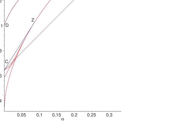
Figure 11: All the curves in Figure 10 are shown, for $0\leq\alpha\leq\frac{1}{3}$, along with the purple line CN and the brown curve DN. The maximum of the three red curves is the best value for the $C_{1,1}$ capacity we have found. The line CN is the capacity of the first adaptive strategy discussed in in this section. The line CZ is the capacity of the second adaptive strategy. The curve DN is the $C_{1,\infty}$ capacity (i.e., the Holevo bound).

Once we have decoded the first stage code, the uncertainty about which codeword we sent is reduced to decoding the second stage code. Because the second code is binary, the decoding of the first-stage code leaves in each position only two possible trines consistent with this decoding. This means that in the approximately $(1-3\alpha)n$ positions where the trines are projected into the plane, we now need only distinguish between two of the three possible trines. In these positions, we can use the optimal measurement for distinguishing between two planar trine states; recall that this is a von Neumann measurement which gives $1-H(1/2+\sqrt{3}/4)=0.64542$ bits of information per position. In the approximately $3\alpha n$ remaining positions, we still know which outcome $D_{b}$ was obtained in the first round of measurements, and this outcome tells us exactly which trine was sent. Decoding the first-stage code left us with two equally likely possibilities in the second-stage code for each of these positions. We thus obtain one bit of information about the second-stage code for each of these approximately $3\alpha$ positions. Thus, if we set $\tau_{2}=0.64542(1-3\alpha)+3\alpha$ bits, by Shannon’s theorem there is a classical error-correcting code which can be used for the second stage and which can almost certainly be decoded uniquely. Adding $\tau_{1}$ and $\tau_{2}$, we obtain a channel capacity of $0.64542(1-3\alpha)+(\log_{2}3)(3\alpha)$ bits; this is the line which interpolates between the points $\alpha=0$ and $\alpha=1/3$ on the curve for $C_{1,1}$. As can be seen from Figure 11, for small $\alpha$ this strategy indeed does better than our best protocol for $C_{1,1}$.

The above strategy can be viewed in a slightly different way, this time as a three-step process. In the first step our measurement either lifts the three trine states up until they are all orthogonal, or projects them into the plane. This first step lifts approximately $3\alpha n$ trines up and projects approximately $(1-3\alpha)n$ trines into the plane. After this first step, we first measure the trines that are lifted further out of the plane, yielding $\log_{2}3$ bits of information for each of these approximately $3\alpha n$ positions. The rest of the strategy then proceeds exactly as above. Note that this reinterpretation of the strategy is reminiscent of the two-stage description of the six-outcome POVM for accessible information in Section 2.

We now modify the above protocol to give the best protocol we currently know for the adaptive capacity $C_{1,A}$. We first make a measurement which either projects the trines $T(\alpha)$ to the planar trines $T(0)$ or lifts them out of the plane to some fixed height, yielding the trines $T(\gamma_{2})$; this measurement requires $\alpha<\gamma_{2}$. (Our first strategy is obtained by setting $\gamma_{2}=\frac{1}{3}$.) We choose $\gamma_{2}=0.087247$; this is the point where the convex hull of the curve representing the $C_{1,1}$ capacity meets this curve (see Figure 10); at this point $C_{1,1}$ is 1.03126 bits. It is easy to verify that with probability $1-\alpha/\gamma_{2}$, the lifted trine $T_{b}(\alpha)$ is projected onto a planar trine $T_{b}(0)$, and with probability $\alpha/\gamma_{2}$, it is lifted up to $T_{b}(\gamma_{2})$. We next use the optimum von Neumann measurement $V(0)=Q(2/3)$ on the trine states that were lifted out of the plane.

We now analyze this protocol in more detail. Let

$$p=\langle V_{b}(0)|T_{b}(\gamma_{2})\rangle^{2}=0.90364.$$ (19)

The first-stage code gives an information gain of

$$\log_{2}3-H(\frac{1+p}{4};\frac{1+p}{4};\frac{1-p}{2})=0.35453\ \mathrm{bits}$$

for each of the approximately $(\alpha/\gamma_{2})n$ signals which were lifted out of the plane. This is because the symbol $a$ in the first-stage code is first taken to $T_{a}$ or $T_{a+1\ ({\mathrm{mod}}\ 3)}$ with a probability of $\frac{1}{2}$ each (depending on the value of the corresponding letter in the second-stage code). We thus obtain each of the two outcomes $V_{a}$, $V_{a+1\ ({\mathrm{mod}}\ 3)}$ with probabilities $\frac{1}{2}p+\frac{1}{2}(1-p)/2=\frac{1}{4}(1+p)$, and obtain the outcome $V_{a+2\ {(\mathrm{mod}}\ 3)}$ with probability $\frac{1}{2}(1-p)$. Thus, if we start with the symbol $a$ in the first-stage code, the entropy of the outcome of the measurement (i.e., $H(X_{\mathrm{out}}|X_{\mathrm{in}})$) is $H(\frac{1+p}{4};\frac{1+p}{4};\frac{1-p}{2})$; it is easy to see that $H(X_{\mathrm{out}})$ is $\log_{2}3$. From classical Shannon theory, we find that we can take $\tau_{1}=0.35453(\alpha/\gamma_{2})$.

The design of our codewords ensures that knowledge of the first codeword eliminates one of the three signal states for each of the trines projected into the plane. This allows us to use the optimal $C_{1,1}$ measurement on the planar trines, resulting in an information gain of 0.64542 bits for each of these approximately $(1-\alpha/\gamma_{2})n$ signals. We obtain

$$\frac{1}{2}(1+p)\left[1-H\left(\frac{1-p}{1+p}\right)\right]=0.67673\quad\mathrm{bits}$$

for each of the approximately $\alpha/\gamma_{2}$ signals that were lifted out of the plane; this will be explained in more detail later. Put together, this results in a capacity of

$$C_{1,A}=0.64542(1-\alpha/\gamma_{2})+1.03126(\alpha/\gamma_{2})$$ (20)

bits per signal; this formula linearly interpolates between the $C_{1,1}$ capacity for $T(0)$ and the $C_{1,1}$ capacity for $T(\gamma_{2})$.

Why do we get the weighted average of $C_{1,1}$ for $T(0)$ and $C_{1,1}$ for $T(\gamma_{2})$ as the $C_{1,1}$ for $T(\alpha)$, $0<\alpha<\gamma_{2}$? This happens because we use all the information that was extracted by both of the measurements. The measurements on the trines that were projected onto the plane only give information about the second code, and provide 0.64542 bits of information per trine. For the trines $T(\gamma_{2})$ that were lifted out of the plane, we use part of the information extracted by their measurements to decode the first code, and part to decode the second code. For these trines, in the first step, we start with the symbols $\{0,1,2\}$ of the first stage code with equal probabilities. A 0 symbol gives measurement outcome $V_{0}$ with probability $\frac{1+p}{4}$, $V_{1}$ with probability $\frac{1+p}{4}$, and $V_{2}$ with probability $\frac{1-p}{2}$, and similarly for the other signals. The information gain from this step is thus

$$\log_{2}3-H\left({\textstyle\frac{1+p}{4};\frac{1+p}{4};\frac{1-p}{2}}\right)=0.35453\quad\mathrm{bits}$$ (21)

per signal. At the start of the second step, we have narrowed the possible states for each signal down to two equally likely possibilities. This information gain for this step comes from the case where the outcome of the measurement was $V_{b}$, and where one of the two possible states (consistent with the first-stage code) is $T_{b}$. This happens with probability $\frac{1}{2}(1+p)$. In this case, we obtain a binary symmetric channel with crossover probability $2p/(1+p)$. In the other case, where the measurement was $V_{b}$ and neither of the two possible states consistent with the first-stage code is $b$, we gain no additional information, since both possible states remain equally likely. The information gain from the second step is thus

$${\textstyle\frac{1}{2}}(1+p)\left[1-H\left(\frac{2p}{1+p}\right)\right]=0.67673\ \mathrm{bits}$$ (22)

per signal. Adding the information gains from the first two stages [Eqs. (21) and (22)] together gives

$$\log_{2}3-H\left({\textstyle p;\frac{1-p}{2};\frac{1-p}{2}}\right),$$ (23)

which is the full information gain from the measurement on the trine states that were lifted further out of the plane; that this happens is, in some sense, an application of the chain rule for classical entropy [2].

,

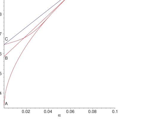
Figure 10: The three red curves AZ, BZ and CZ are all shown in Fig. 6; their maximum is the best value known for $C_{1,1}$ capacity. The blue line CZ is straight; it is the second adaptive strategy discussed in this section, and is the largest value we know how to obtain for $C_{1,A}$.

,

5 The upper bound on $C_{1,1}$

In this section, we show that for the lifted trines $T(\alpha)$, if $\alpha$ is small, then the $C_{1,A}$ capacity is exponentially close to the accessible information obtainable using just two of our trines, showing that the three red curves in Fig. 6 are exponentially close when $\alpha$ is close to 0.

First, we need to prove that in a classical channel, changing the transition probabilities by $\epsilon$ can only change the Shannon information by $O(-\epsilon\log_{2}\epsilon)$. The Shannon capacity of a classical channel with input distribution $p_{i}$ and transition probabilities $q_{ij}$ is the entropy of the output less the entropy of the output given the input, or

$$I_{S}=-\sum_{j=0}^{N_{\rm out}-1}\left(\sum_{i=0}^{N_{\rm in}-1}p_{i}q_{ij}\right)\log_{2}\sum_{i=0}^{N_{\rm in}-1}p_{i}q_{ij}+\sum_{i=0}^{N_{\rm in}-1}\sum_{j=0}^{N_{\rm out-1}}p_{i}q_{ij}\log_{2}q_{ij}.$$ (24)

Suppose we change all the $q_{ij}$ by at most $\epsilon$. I claim that the above expression changes by at most $-2N_{\rm out}\,\epsilon\log_{2}\epsilon$. Each of the terms $q_{ij}\log_{2}q_{ij}$ in the second term changes by at most $-\epsilon\log_{2}\epsilon$, and adding these changes (with weights $p_{i}$) gives a total change of at most $-N_{\rm out}\epsilon\log_{2}\epsilon$. Similarly, each of the terms $\sum_{i}p_{i}q_{ij}$ in the first term of (24) changes by at most $\epsilon$, and there are at most $N_{\rm out}$ of them, so we see easily that the first term also contributes at most $-N_{\rm out}\epsilon\log_{2}\epsilon$ to the change. For $N_{\rm out}\leq 6$, which by the real version of Davies’ theorem is sufficient for the optimum measurement on the lifted trines, we have that the change is at most $-12\epsilon\log_{2}\epsilon$.

Next, we need to know that the $C_{1,1}$ capacity for the planar trines is maximized using the probability distribution $(0,\frac{1}{2},\frac{1}{2})$, One can easily convince oneself of this by inspecting Figure 14. We will discuss this at more length in Appendix A, where we sketch a proof that the point $(0,\frac{1}{2},\frac{1}{2})$ is a local maximum for the accessible information. The proof also shows that to achieve a capacity close to $C_{1,1}$ one must use a probability distribution and measurement close to those achieving the optimal, a fact we will be using in this section.

Now, we can deal with lifted trines. We will consider the trine states $T(\alpha)$ for small $\alpha$. By moving each of the trines $T(\alpha)$ by an angle of $\phi=\arcsin\sqrt{\alpha}<2\sqrt{\alpha}$, we can obtain the planar trines $T(0)$. We now have that the difference between the transition probabilities for $T(\alpha)$ and $T(0)$ for any rank 1 element in a POVM is at most $\phi$, since the transition probability for a fixed POVM element $r\left|\,v\right\rangle\!\!\left\langle v\,\right|$ is a constant multiple (with the constant being $r\leq 1$) of the square of the cosine of the angle between the vectors $\left|\,v\right\rangle$ and $\left|\,T_{b}\right\rangle$, and this angle changes by at most $\phi$. Thus, by the lemma above, the $C_{1,1}$ capacity for the lifted trines $T(\alpha)$ differs by no more than $\delta=-12{\phi}\log_{2}{\phi}$ from the capacity obtained when the same probabilities (and measurement) are used for the planar trine states $T(0)$.

For the lifted trine states $T(\alpha)$, we know (from Section 3) that the $C_{1,1}$ capacity $C_{1,1}(\alpha)$ is greater than $C_{1,1}(0)$, the capacity for the planar trine states. If we apply to the planar trine states $T(0)$ the same measurements and the same probability distribution that give the optimum $C_{1,1}$ capacity for the lifted trine states $T(\alpha)$, we know that we have changed the capacity by at most $\delta=-12\phi\log_{2}\phi$. We thus have that $C_{1,1}(0)<C_{1,1}(\alpha)<C_{1,1}(0)+\delta$, and that the measurements and probability distribution that yield the optimum capacity $C_{1,1}(\alpha)$ for the lifted trines $T(\alpha)$ must give a capacity of at most $C_{1,1}(0)-\delta$ when applied to the planar trines. This limits the probability distribution and measurement giving the optimum capacity $C_{1,1}$ for the lifted trines. For sufficiently small $\alpha$, the optimum probability distribution on the trines must be close to $(0,\frac{1}{2},\frac{1}{2})$, and when the optimum projectors are projected onto the plane, nearly all the mass must be contained in projectors within a small angle of the optimum projectors for $C_{1,1}(0)$, namely $\frac{1}{\sqrt{2}}(1,\pm 1)$.

We now consider the derivative in the information capacity obtained when the measurement is held fixed, and $p_{0}$ is increased at a rate of 1 while $p_{1}$ and $p_{2}$ are decreased, each at a rate of $1/2$. Taking the derivative of (24), we obtain

$$I_{S}^{\prime}=-\sum_{j=0}^{5}\left(\sum_{i=0}^{2}p^{\prime}_{i}q_{ij}\right)\log_{2}\sum_{i=0}^{2}p_{i}q_{ij}+\sum_{i=0}^{2}\sum_{j=0}^{5}p^{\prime}_{i}q_{ij}\log_{2}q_{ij},$$ (25)

where $p_{0}^{\prime}=1$ and $p_{1}^{\prime}=p_{2}^{\prime}=-1/2$. This derivative can be broken into terms associated with each of the projectors in the measurement. Namely, if the $j$th POVM element is ${r_{j}}\left|\,v\right\rangle\!\!\left\langle v\,\right|$, then the associated term is

$$-r_{j}\left(\sum_{i=0}^{2}p^{\prime}_{i}q_{iv}\right)\log_{2}\sum_{i=0}^{2}p_{i}q_{iv}+r_{j}\sum_{i=0}^{2}p^{\prime}_{i}q_{iv}\log_{2}q_{iv},$$

where $q_{iv}=|\langle T_{i}|v\rangle|^{2}$, $p_{0}^{\prime}=1$ and $p_{1}^{\prime}=p_{2}^{\prime}=-1/2$. The $r_{j}$ can be factored out, and this term can be written as $r_{j}I^{\prime}_{v}$ where we define

$$I_{v}^{\prime}=-\left(\sum_{i=0}^{2}p^{\prime}_{i}q_{iv}\right)\log_{2}\sum_{i=0}^{2}p_{i}q_{iv}+\sum_{i=0}^{2}p^{\prime}_{i}q_{iv}\log_{2}q_{iv}.$$ (26)

It is easy to see that for the planar trines, a projector $v_{\theta}=(\cos\theta,\sin\theta)$ with $\theta$ sufficiently close to $\pm\pi/4$, and a probability distribution sufficiently close to $(0,\frac{1}{2},\frac{1}{2})$, the term $I^{\prime}_{v_{\theta}}$ is approximately $-0.3227$ bits, the value of $I_{v_{\theta}}^{\prime}$ at $\theta=\pm\pi/4$ and the probability distribution $(0,\frac{1}{2},\frac{1}{2})$. Similarly, for the planar trines, if the probability distribution is close to $(0,\frac{1}{2},\frac{1}{2})$, $I_{v_{\theta}}^{\prime}$ can never be much greater than $2$ bits, which is the maximum value for the probability distribution $(0,\frac{1}{2},\frac{1}{2})$ (occurring at $\theta=0$). These facts show that if $\alpha$ is sufficiently small, then the formula (25) for the derivative of the accessible information is negative and bounded above by (say) $-0.64$ bits when the planar trines are measured with the optimum POVM for $C_{1,1}(\alpha)$. This is true because $\sum_{j}r_{j}=2$, and all but a $1-\epsilon$ fraction of the mass must be in projectors $v_{\theta}$ for $\theta$ near $\pm\pi/4$; each of these projectors will contribute at least $0.321r_{j}$ (say) to the derivative, and the projectors with $\theta$ not near $\pm\pi/4$ cannot change this result by more than $4\epsilon$. For the optimum measurement and probability distribution for $C_{1,1}(\alpha)$ to have a non-zero value of $p_{0}$ (from Section 3 we know it does), this negative derivative must be balanced by a positive derivative acquired by some projectors when the trines are lifted out of the plane. We will show that this can only happen when $p_{0}$ is exponentially small in $1/\delta$; for larger values of $p_{0}$, the positive component acquired when the trines are lifted out of the plane is dwarfed by the negative component retained from the planar trines.

We have shown that $I_{S}^{\prime}<-0.64$ bits near the probability distribution $(0,\frac{1}{2},\frac{1}{2})$ when the optimal measurement for $T(\alpha)$ is applied to the planar trines, assuming sufficiently small $\alpha$. We also know from the concavity of the mutual information that for the lifted trines $T(\alpha)$ with $\alpha>0$, the derivative $I_{S}^{\prime}$ is positive for any probability distribution $(p_{0}-t,p_{1}+t/2.p_{2}+t/2)$ where $(p_{0},p_{1},p_{2})$ is the optimal probability for $C_{1,1}$ capacity and $0<t\leq p_{0}$. Thus, we know that the negative derivative for the planar trines must be balanced by a positive derivative acquired by some projectors when you consider the difference between the planar trines and the lifted trines. We will show that this can only happen when the probability $p_{0}$ is exponentially small in the lifting angle $\phi$. This shows that at the probability distribution achieving $C_{1,1}$, $p_{0}$ is exponentially small in $1/\phi=1/\arcsin\sqrt{\alpha}$.

Consider the change in the derivative $I_{v_{j}}^{\prime}$ for a given projector $v_{j}$ when the trines $T(0)$ are lifted out of the plane to become the trines $T(\alpha)$. To make $I_{v_{j}}^{\prime}$ positive, this change must be at least $0.64$ bits. Let the transition probabilities with the optimal measurement for $C_{1,1}(\alpha)$ be $r_{j}q_{iv_{j}}$ and the transition probabilities for the same measurement applied to the planar trines be $r_{j}\tilde{q}_{iv_{j}}$. Since the constant factors $r_{j}$ multiplying the projectors sum to $3$, we have that the value $I_{v}^{\prime}$ for one projector $v$ must change by at least $0.21$ bits, that is,

$$\left|\left(\sum_{i=0}^{2}p^{\prime}_{i}\tilde{q}_{iv}\right)\log_{2}\sum_{i=0}^{2}p_{i}\tilde{q}_{iv}\right. - \left(\sum_{i=0}^{2}p^{\prime}_{i}q_{iv}\right)\log_{2}\sum_{i=0}^{2}p_{i}q_{iv}$$

$$\left.\quad+\sum_{i=0}^{2}p^{\prime}_{i}\left(q_{iv}\log_{2}q_{iv}-\tilde{q}_{iv}\log_{2}\tilde{q}_{iv}\right)\right|>0.21$$

where $\tilde{q}_{iv}=|\langle T_{i}(0)|v\rangle|^{2}$ and ${q}_{iv}=|\langle T_{i}(\alpha)|v\rangle|^{2}$, as before. We know $|\tilde{q}_{iv}-q_{iv}|\leq\phi$.

We will first consider the last term of (5),

$$\left|\sum_{i=0}^{2}\sum_{j=0}^{5}p^{\prime}_{i}(q_{iv}\log_{2}q_{iv}-\tilde{q}_{iv}\log_{2}\tilde{q}_{iv})\right|$$

This is easily seen to be bounded by $-6\phi\log_{2}\phi$, which approaches $0$ as $\alpha$ approaches $0$.

Next, consider the first terms of (5),

$$\left|\left(\sum_{i=0}^{2}p^{\prime}_{i}q_{iv}\right)\log_{2}\sum_{i=0}^{2}p_{i}{q}_{iv}-\left(\sum_{i=0}^{2}p^{\prime}_{i}\tilde{q}_{iv}\right)\log_{2}\sum_{i=0}^{2}p_{i}\tilde{q}_{iv}\right|.$$ (27)

Bounding this is a little more complicated. First, we will derive a relation among the values of $\tilde{q}_{iv}$ for different $i$. We use the fact that for the planar trines

$$\left|\,T_{0}(0)\right\rangle=-\left|\,T_{1}(0)\right\rangle-\left|\,T_{2}(0)\right\rangle.$$

Taking the inner product with $\left\langle v_{j}\,\right|$, we get

$$\langle v_{j}|T_{0}(0)\rangle=-\langle v_{j}|T_{1}(0)\rangle-\langle v_{j}|T_{2}(0)\rangle.$$

And now, using the fact that $\tilde{q}_{iv}=|\langle v_{j}|T_{i}(0)\rangle|^{2}$, we see that

$$\tilde{q}_{0v}\leq 2(\tilde{q}_{1v}+\tilde{q}_{2v}).$$ (28)

Using (28), and the fact that $p_{1},p_{2}$ are close to $\frac{1}{2}$, we have that

$$\sum_{i=0}^{2}p_{i}\tilde{q}_{iv} \geq \frac{3}{8}\tilde{q}_{1v}+\frac{3}{8}\tilde{q}_{2v}$$ (29)

$$\geq \frac{1}{8}(\tilde{q}_{0v}+\tilde{q}_{1v}+\tilde{q}_{2v})$$

for sufficiently small $\alpha$. We also need a relation among the $q_{iv}$. We have

$$q_{0v}+q_{1v}+q_{2v} = \left\langle v\,\right|\Big{(}\sum_{i=0}^{2}\left|\,T_{i}\right\rangle\!\!\left\langle T_{i}\,\right|\Big{)}\left|\,v\right\rangle$$ (30)

$$\geq \frac{1}{4}\phi^{2},$$

where the second step follows because the minimum eigenvalue of $\left|\,T_{0}\right\rangle\!\!\left\langle T_{0}\,\right|+\left|\,T_{2}\right\rangle\!\!\left\langle T_{2}\,\right|+\left|\,T_{2}\right\rangle\!\!\left\langle T_{2}\,\right|$ is $\alpha>\phi^{2}/4$.

We now are ready to bound the formula (5). We break it into two pieces; if this expression is at least 0.2 bits, then one of these two pieces must be at least 0.1 bits. The two pieces are as follows:

$$\left|\left(\sum_{i=0}^{2}p^{\prime}_{i}(q_{iv}-\tilde{q}_{iv})\right)\log_{2}\sum_{i=0}^{2}p_{i}{q}_{iv}\right|$$ (31)

and

$$\left|\left(\sum_{i=0}^{2}p^{\prime}_{i}\tilde{q}_{iv}\right)\left(\log_{2}\sum_{i=0}^{2}p_{i}{q}_{iv}-\log_{2}\sum_{i=0}^{2}p_{i}\tilde{q}_{iv}\right)\right|.$$ (32)

We first consider the case of (31). Assume that it is larger than $0.1$ bits. Then

$$\left|\left(\sum_{i=0}^{2}p^{\prime}_{i}(q_{iv}-\tilde{q}_{iv})\right)\log_{2}\sum_{i=0}^{2}p_{i}{q}_{iv}\right| \leq -\left(\sum_{i=0}^{2}|p_{i}^{\prime}|\phi\right)\log_{2}\sum_{i=0}^{2}p_{0}q_{iv}$$ (33)

$$\leq -2\phi\log_{2}\frac{p_{0}\phi^{2}}{4}$$ (34)

where the first step follows from the facts that $|q_{iv}-\tilde{q}_{iv}|<\phi$ and that $p_{0}$ is the smallest of the $p_{i}$, and the second step follows from (30). Thus, if the quantity (31) is at at least $0.1$, we have that

$$p_{0}<\frac{4}{\phi^{2}}2^{-0.05/\phi}$$

showing that $p_{0}$ is exponentially small in $1/\phi$.

We next consider the case (32). Assume that

$$\left|\left(\sum_{i=0}^{2}p^{\prime}_{i}\tilde{q}_{iv}\right)\left(\log_{2}\sum_{i=0}^{2}p_{i}{q}_{iv}-\log_{2}\sum_{i=0}^{2}p_{i}\tilde{q}_{iv}\right)\right|$$

is larger than $0.1$ bits. We know that

$$\left|\sum_{i=0}^{2}p^{\prime}_{i}\tilde{q}_{iv}\right|\leq\sum_{i=0}^{2}|p^{\prime}_{i}|=2$$

Thus, for (32) to be larger than $0.1$, we must have that

$$\left|\log_{2}\frac{\sum_{i=0}^{2}p_{i}q_{iv}}{\sum_{i=0}^{2}p_{i}\tilde{q}_{iv}}\right|>0.05\,.$$

We know that the numerator and denominator inside the logarithm differ by at most $\phi$. It is easy to check that if $|\log_{2}(x/y)|>0.05$, and $x-y\leq\phi$, then both $x$ and $y$ are at most $15\phi$. Thus,

$$\sum_{i=0}^{2}p_{i}\tilde{q}_{iv}<15\phi.$$ (35)

Further,

$$\left|\sum_{i=0}^{2}p^{\prime}_{i}\tilde{q}_{iv}\right| \leq \sum_{i=0}^{2}\tilde{q}_{iv}$$

$$\leq 8\sum_{i=0}^{2}p_{i}\tilde{q}_{iv}$$

$$\leq 120\phi.$$

where the second inequality follows by (29) and the third by (35).

Since the two terms in (32) are of opposite signs, if they add up to at least 0.1 bits, at least one of them must exceed $0.1$ bits by itself. We will treat these two cases separately. First, assume that the first term exceeds $0.1$. Then

$$0.1 \leq -\left|\sum_{i=0}^{2}p_{i}^{\prime}\tilde{q}_{iv}\right|\log_{2}\sum_{i=0}^{2}p_{i}q_{iv}$$

$$\leq -\left|\sum_{i=0}^{2}p_{i}^{\prime}\tilde{q}_{iv}\right|\log_{2}\sum_{i=0}^{2}p_{0}q_{iv}$$

$$\leq -120\phi\log_{2}\frac{p_{0}\phi^{2}}{4},$$

where the last inequality follows from (30) and (5). If this is at least $0.1$, then we again have that $p_{0}$ is exponentially small in $1/\phi$.

Finally, we consider the case of the term

$$-\left|\sum_{i=0}^{2}p_{i}^{\prime}\tilde{q}_{iv}\right|\log_{2}\sum_{i=0}^{2}p_{i}\tilde{q}_{iv}.$$

We have by (29) that

$$-\left|\sum_{i=0}^{2}p_{i}^{\prime}\tilde{q}_{iv}\right|\log_{2}\sum_{i=0}^{2}p_{i}\tilde{q}_{iv}\leq-\left(\sum_{i=0}^{2}\tilde{q}_{iv}\right)\log_{2}\frac{1}{8}\sum_{i=0}^{2}\tilde{q}_{iv},$$

which, since $\sum_{i=0}^{2}\tilde{q}_{iv}<120\phi$, can never exceed $0.1$ for small $\phi$, as it is of the form $-8x\log x$ for a small $x$.

Since $p_{0}$ is exponentially small in $1/\phi$, we have that the difference between the $C_{1,1}$ capacity using only two trines and that using all three trines is exponentially small in $\frac{1}{\sqrt{\alpha}}$, showing that our guess in Section 3 are exponentially close to the correct $C_{1,1}$ capacity as $\alpha$ goes to $0$, and thus showing that $C_{1,A}$ is strictly larger than $C_{1,1}$ in a region near $\alpha=0$.

6 $C_{1,1}=C_{1,A}$ for two pure states

In this section, we prove that for two pure states, $C_{1,1}=C_{1,A}$. We do this by giving a general upper bound on $C_{1,A}$ based on a tree construction, We then use the fact that for two pure states, accessible information is concave in the probabilities of the states (proved in Appendix B) to show that this upper bound is equal to $C_{1,1}$ for ensembles containing only two pure states.

For the upper bound, we consider a class of trees, with an ensemble of states associated with each node. The action of Bob’s measurement protocol on a specific signal will generate such a tree, and analyzing this tree will bound the amount of information Bob can on average extract from that signal. Associated with each tree will be a capacity, and the supremum over all trees will give an upper bound for $C_{1,A}$.

We now describe our tree construction in general. Let us suppose that Alice can convey to Bob one of $m$ possible signal states. Let these states be $\rho_{i}$, where $1\leq i\leq m$. To each tree node we assign $m$ density matrices and $m$ associated probabilities (these will not be normalized, and so may sum to less than 1). For node ${\bf x}$ of the tree, we associate some POVM element $E_{\bf x}$, and the $m$ density matrices $E_{\bf x}^{1/2}\rho_{i}E_{\bf x}^{1/2}/\mbox{\rm\/Tr }E_{\bf x}\rho_{i}$, where $\rho_{i}$ are the original signal states. (We may omit the normalization factor of $\mbox{\rm\/Tr }E_{\bf x}\rho_{i}$ in this discussion when it is clear from context.) For the root node ${\bf r}$, the POVM element $E_{\bf r}$ is the identity matrix $I$, and the probability $p_{{\bf r},i}$ is the probability that this signal is $\rho_{i}$. A probability $p_{\bf x}$ can be associated with node ${\bf x}$ by summing $p_{\bf x}=\sum_{i=1}^{m}p_{{\bf x},i}$. For the root, $p_{\bf r}=1$. For any node ${\bf x}$, its associated probability $p_{\bf x}$ will be equal to the sum of the probabilities $p_{{\bf y}_{j}}$ associated with its children ${\bf y}_{j}$. There are two classes of nodes, distinguished by the means of obtaining its children from the node. The first class we call measurement nodes and the second we call probability refinement (or refinement) nodes. For a measurement node $\bf x$, we assign to each of the children ${\bf y}_{j}$ a POVM elements $E_{{\bf y}_{j}}$, where $\sum_{j}E_{{\bf y}_{j}}=E_{\bf x}$. The density matrices associated with a child of ${\bf x}$ will be $E_{{\bf y}_{j}}^{1/2}\rho_{i}E_{{\bf y}_{j}}^{1/2}/\mbox{\rm\/Tr }E_{{\bf y}_{j}}\rho_{i}$, and the probability associated with the density matrix $E_{{\bf y}_{j}}^{1/2}\rho_{i}E_{{\bf y}_{j}}^{1/2}/\mbox{\rm\/Tr }E_{{\bf y}_{j}}\rho_{i}$ will be $p_{{\bf y}_{j},i}=p_{{\bf x},i}\mbox{\rm\/Tr }(E_{{\bf y}_{j}}\rho_{i})/\mbox{\rm\/Tr }(E_{\bf x}\rho_{i})$. Finally, we define the information gain associated with a node ${\bf x}$. This is $0$ for nodes which are not measurement nodes, and

$$I_{\bf x}=p_{\bf x}H\left(\left\{\frac{p_{{\bf x},i}}{p_{\bf x}}\right\}\right)-\sum_{k}p_{{\bf y}_{k}}H\left(\left\{\frac{p_{{\bf y}_{k},i}}{p_{{\bf y}_{k}}}\right\}\right),$$

where $H(\{q_{i}\})$ is the Shannon information $\sum_{i}q_{i}\log_{2}q_{i}$ of the probability distribution $\{q_{i}\}$.

We now explain why we chose this formula. We consider applying a measurement to the ensemble associated with node ${\bf x}$. This ensemble contains the state $E_{\bf x}^{1/2}\rho_{i}E_{\bf x}^{1/2}/\mbox{\rm\/Tr }(\rho_{i}E_{\bf x})$ with probability $p_{{\bf x},i}/p_{\bf x}$. Let us apply the measurement that takes $\rho$ to $A_{k}\rho A_{k}^{{\dagger}}$ with probability $\mbox{\rm\/Tr }A_{k}^{\dagger}A_{k}\rho_{i}$, where $\sum_{k}A_{k}^{\dagger}A_{k}=I$. Each child ${\bf y}_{k}$ of ${\bf x}$ is associated with one of the matrices $A_{k}$. Let $E_{{\bf y}_{k}}=E_{\bf x}^{1/2}A_{k}^{\dagger}A_{k}E_{\bf x}^{1/2}$. Then $\sum_{k}E_{{\bf y}_{k}}=E_{\bf x}$. Now, after we apply $A_{k}$ to $E_{\bf x}^{1/2}\rho_{i}E_{\bf x}^{1/2}$, we obtain the state $A_{k}E_{\bf x}\rho_{i}E_{\bf x}A_{k}^{\dagger}$. This happens with probability

$$\frac{\mbox{\rm\/Tr }A_{k}E_{\bf x}^{1/2}\rho_{i}E_{\bf x}^{1/2}A_{k}^{{\dagger}}}{\mbox{\rm\/Tr }E_{\bf x}\rho_{i}}=\frac{\mbox{\rm\/Tr }E_{{\bf y}_{k}}\rho_{i}}{\mbox{\rm\/Tr }E_{\bf x}\rho_{i}}.$$

The state we obtain, $A_{k}E_{\bf x}^{1/2}\rho_{i}E_{\bf x}^{1/2}A_{k}^{\dagger}$, is unitarily equivalent to $E_{{\bf y}_{k}}^{1/2}\rho_{i}E_{{\bf y}_{k}}^{1/2}$, so this latter state can be obtained by an equivalent measurement. The information $I_{\bf x}$ associated with the node $\bf x$ is the probability of reaching the node times the Shannon information gained by this measurement if the node is reached. Summing $I_{\bf x}$ over all the nodes ${\bf x}$ of the tree gives the expected information gain by measurement steps.

The second class of nodes are probability refinement nodes (which we often shorten to refinement nodes). Here, for all the children $\{{\bf y}_{k}\}$ of ${\bf x}$, $E_{\bf x}=E_{{\bf y}_{k}}$. We assign probabilities $p_{{\bf y}_{k},i}$ to the children ${\bf y}_{k}$ so that $\sum_{k}p_{{\bf y}_{k},i}=p_{{\bf x},i}$. For this class of nodes, we define $I_{\bf x}$ to be $0$. These nodes correspond to steps in the protocol where additional information is gained about one signal state in the codeword by measuring different signal states in the codeword.

To find the upper bound on the $C_{1,1}$ capacity for a set of states $\{\rho_{i}\}$, we take the supremum over the information gain associated with all trees of the above form. That is, we try to maximize $\sum_{\bf x}I_{\bf x}$ over all probability distributions $p_{{\bf r},i}$ on the root node ${\bf r}$, all ways of splitting $E_{\bf x}=\sum_{k}E_{{\bf y}_{k}}$ for measurement nodes ${\bf x}$, and all ways of splitting probabilities $p_{{\bf x},i}=\sum_{k}p_{{\bf y}_{k},i}$ for refinement nodes ${\bf x}$ and signal states $i$. (And if this maximum is not attained, we take the supremum.)

To prove this upper bound, we track the information obtained from a single signal (i.e., channel output) $S_{\nu}$ in the protocol used by Alice and Bob. We assume that Alice sends Bob a set of states, and Bob performs measurements on them one at a time. We keep track at all times $t$ (i.e., for all nodes x of the tree) of the probability that signal $S_{\nu}$ is in state $E_{\bf x}^{1/2}\rho_{i}E_{\bf x}^{1/2}$. There are two cases, depending on which signal Bob measures. In the first case, when Bob measures signal $S_{\nu}$, we perform a measurement on the current tree node $\bf x$ that splits each of the possible values of $\rho_{t,i}$ for this signal $S_{\nu}$ into several different values. This case corresponds to a measurement node of the tree. We can assume without loss of generality that for his measurement Bob uses the canonical type of operators discussed above, so that $E_{\bf x}^{1/2}\rho_{i}E_{\bf x}^{1/2}$ goes to $E_{{\bf y}_{k}}^{1/2}\rho_{i}E_{{\bf y}_{k}}^{1/2}$ with probability $\mbox{\rm\/Tr }E_{{\bf y}_{k}}\rho_{i}/\mbox{\rm\/Tr }E_{\bf x}\rho_{i}$. Thus, we now have several different ensembles of density matrices, the $k$th of which contains $E_{{\bf y}_{k}}^{1/2}\rho_{i}E_{{\bf y}_{k}}^{1/2}/\mbox{\rm\/Tr }E_{{\bf y}_{k}}\rho_{i}$ with (unnormalized) probability $p_{{\bf x},i}\mbox{\rm\/Tr }E_{{\bf y}_{k}}\rho_{i}/\mbox{\rm\/Tr }E_{{\bf x}}\rho_{i}=p_{{\bf y}_{k},i}$. In this step Bob can extract some information about the original codeword, and the amount of this information is at most $I_{\bf x}$.

The other case comes when Bob measures signals than $S_{\nu}$. These steps can provide additional information about the signal $S_{\nu}$, so if the probability distribution before this step contained $E_{\bf x}^{1/2}\rho_{i}E_{\bf x}^{1/2}$ with probability $p_{{\bf x},i}$, we now have several distributions, each assigned to a child of ${\bf x}$; the $j$th distribution contains $E_{\bf x}^{1/2}\rho_{i}E_{\bf x}^{1/2}$ with (unnormalized) probability $p_{{\bf y}_{j},i}$ Here, we must have $\sum_{j}p_{{\bf y}_{j},i}=p_{{\bf x},i}$. This kind of step corresponds to a probability refinement node in the tree. The information gained by these measurement steps can be attributed to the signals that are actually measured in these steps, so we need not attach any information gain to the refinement steps in the tree formulation. Averaging the information gain over the trees associated with all the signals gives the capacity of the protocol, which is the expected information gain per signal sent.

There are several simplifying assumptions we can make about the trees. First, we can assume that nodes just above leaves are measurement nodes that contain only rank 1 projectors, since any refinement node having no measurement nodes below it can be eliminated without reducing the information content of the tree, and since the last measurement might as well extract as much information as possible. We could assume that the types of the nodes are alternating, since two nodes of the same type, one a child of the other, can be collapsed into one node. In the sequel, we will perform this collapse on the measurement nodes, so we assume that all the children of measurement nodes are refinement nodes. We could also (but not simultaneously) assume that every node has degree two, since any measurement with more than two outcomes can be replaced with an equivalent sequence of measurements, each having only two outcomes, and any split in probabilities can be replaced by an equivalent sequence of splits. In the sequel we will assume that all the probability refinement nodes are of degree two.

One interesting question is whether any tree of this form has an associated protocol. The upper bound will hold whether or not this is the case, but if there are trees with no associated protocols, the bound may not be tight. We do not know the answer to this, but suspect that there are trees with no associated protocols. Our (vague) intuition is that if the root node is a measurement node with no associated information gain, and all of the children of this node are refinement nodes, there appears to be no way to obtain the information needed to perform one of these refinement steps without also obtaining the information needed to perform the all the other refinement steps of the root node. However, making this much information available at the top node would reduce the information that could be obtained using later measurement nodes. It is possible that this difficulty can be overcome if there is a feedback channel available from the receiver to the sender. We thus boldly conjecture

Conjecture 1

If arbitrary use of a classical feedback channel from the sender to the receiver is available for free, then the adaptive capacity with feedback $C_{1,AF}$ is given by the supremum over all trees of the above type of the information associated with that tree.

As mentioned above, the supremum of the extractable information over all trees is an upper bound on $C_{1,A}$, since it is at least as large as the information corresponding to any possible adaptive protocol. We now restrict our discussion to the case of ensembles consisting of two pure states, and prove that in this case we have equality, since both of these bounds are equal to the $C_{1,1}$ capacity. Consider a tree which gives a good information gain for this ensemble (we would say maximum, but have no proof that the supremum is obtainable). There must be a deepest refinement node, so all of its descendents are measurement nodes. We may without loss of generality assume that this deepest refinement node has only two children. Each of these two children has an associated ensemble consisting of two pure states with some probabilities. The maximum information tree will clearly assign the optimum measurement to these nodes. However, an explicit expression for this optimum measurement is known [3, 10, 11, 12], and as is proved in Appendix B, the accessible information for ensembles of two given pure states is concave in the probabilities of the states. Thus, if we replace this refinement node with a measurement node, we obtain a tree with a higher associated information value. Using induction, we can perform a series of such steps which do not decrease the information gain associated with the tree while collapsing everything to a single measurement. Thus, for two pure states, we have $C_{1,1}=C_{1,A}$.

The above argument would work to show that $C_{1,1}=C_{1,A}$ for ensembles consisting of two arbitrary density matrices if we could show that the accessible information for two arbitrary density matrices is concave in the probabilities of these two density matrices. It would seem intuitively that this should be true, but we have not been able to prove it. It may be related to the conjecture [11, 4] that the optimal accessible information for two arbitrary density matrices can always be achieved by a von Neumann measurement. This has been proved in two dimensions [11], and is supported by numerical studies in higher dimensions [4]. We thus conjecture:

Conjecture 2

$C_{1,A}=C_{1,1}$ for two mixed states in arbitrary dimensions.

In fact, the proof in this section will work for any upper bound on accessible information which has both the concavity property and the property that if a measurement is made on the ensemble, the sum of the information extracted by this measurement and the expected upper bound for the resulting ensemble is at most the original upper bound. The Fuchs-Caves bound [5] (which was Holevo’s original bound) may have these properties; we have done some numerical tests and have not found a counterexample. For 3 planar trine states with equal probabilities, this gives an upper bound of approximately 0.96.

,

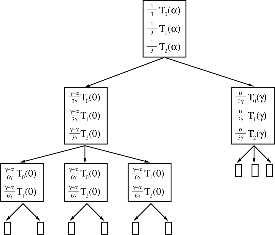
Figure 12: The tree corresponding to the best adaptive protocol of Section 4. To simplify the diagram, we do not give the probabilities and states in the ensembles of the leaves of this tree, which are represented here by empty boxes. Since they are reached by the final measurement, which projects onto a rank 1 density matrix, the quantum states corresponding to these nodes are now completely reduced, and no further information can be extracted from these ensembles. The probabilities can be computed from the discussion in Section 3.

7 Discussion

If we force Bob to measure his signals sequentially, so that he must complete his measurement on signal $k$ before he starts measuring signal $k+1$ (even if he can adaptively choose the order he measures the signals in and even if a feedback channel is applied from Bob to Alice), Bob can never achieve a capacity greater than $C_{1,1}$. This can easily be seen. Without decreasing the capacity, we assume that Bob uses a feedback channel to send all the information that he has back to Alice. This information consists of the results of the measurement and the measurement that he plans to perform next. The ensemble of signals that Alice now sends Bob can convey no more information than the optimal set of signals for this measurement. However, it now follows from classical information theory that such a protocol can never have a capacity greater than the sum of the optimal information gains for all these measurements, which is at most $C_{1,1}$.

It is thus clear that the advantage of adaptive protocols is obtained from the fact that Bob can adjust subsequent measurements of a signal depending on the outcome of the first round of measurements on the entire codeword. In the information decision tree of Section 6 for our protocol (see Figure 12). the crucial fact is that we first either project each of the trine states into the plane or lift it up. We then arrange to distinguish between only two possible states for those signals that were projected into the plane, and among all three possible states for those signals that were lifted.

As we showed in Section 6, $C_{1,1}=C_{1,A}$ for two pure states, and this proof can be extended to apply to two arbitrary states if a very plausible conjecture on the accessible information for a two-state ensemble holds. For three states, even in two dimensions, the same upper bound proof cannot apply. However, for three states in two dimensions, it may still be that $C_{1,1}=C_{1,A}$. We have unsuccessfully tried to find strategies that perform better than the $C_{1,1}$ capacity for the three planar trine states, and we now suspect that the adaptive capacity is the same as the $C_{1,1}$ capacity in this case, and that this is also the case for arbitrary sets of pure states in two dimensions.

Conjecture 3

For an arbitrary set of pure states in two dimensions, $C_{1,1}=C_{1,A}$, and in fact, this capacity is achievable by using as signal states the two pure states in the ensemble with inner product closest to 0.

For general situations, we know very little about $C_{1,A}$. In fact, we have no good criterion for deciding whether $C_{1,A}$ is strictly greater than $C_{1,1}$. Another question is whether entangled inputs could improve the adaptive capacity. That is, whether $C_{1,A}=C_{\infty,A}$, where $C_{\infty,A}$ is the capacity given entangled inputs and single-signal, but adaptive, measurements.

Appendix A: The $C_{1,1}$ capacity for the planar trines

Next, we discuss the $C_{1,1}$ capacity for trines in the plane. For Section 3, we needed to show two things. First, that $C_{1,1}$ for the planar trines was maximized using the probability distribution $\Pi_{2}=(0,\frac{1}{2},\frac{1}{2})$, and second, that any protocol with capacity close to $C_{1,1}$ must use nearly the same probability distribution and measurement as the optimum protocol achieving $C_{1,1}$. We show that in the neighborhood of the probability distribution $\Pi_{2}$, the optimum measurement for accessible information contains only two projectors, From this proof, both facts can be easily deduced; we provide a proof of the first, the second follows easily from an examination of our proof.

We first show that if an optimum measurement for accessible information has only $k$ projectors, then at most $k$ different input states are needed to achieve optimality. This result is a know classical result; for completeness, I provide a brief proof. Shannon’s formula for the capacity of a classical channel is the entropy of the average output less the average entropy of the output. It follows that the number of input states of a classical channel needed to achieve optimality never exceeds the number of output states. If there are $k$ outcomes, and $k^{\prime}>k$ input states, then the output probability distribution can be held fixed on a ($k^{\prime}-k$)-dimensional subspace of the input probability distributions. By the linearity of the average entropy, the minimum average entropy can be achieved at a point of that subspace which has only $k$ non-zero probabilities on the input states. Thus, if the optimal measurement is a von Neumann measurement, only two trines are required to achieve optimality.

We associate to each projector $v_{\theta}=(\cos\theta,\sin\theta)$ an information quantity depending on the probability distribution $\Pi=(p_{0},p_{1},p_{2})$, namely

$$I_{\Pi}(\theta)=-\left(\sum_{i=0}^{2}p_{i}q_{i,\theta}\right)\log_{2}\sum_{i=0}^{2}p_{i}q_{i,\theta}+\sum_{i=0}^{2}p_{i}q_{i,\theta}\log_{2}q_{i,\theta}$$

where $q_{i,\theta}=|\langle T_{i}|v_{\theta}\rangle|^{2}$. The accessible information for a measurement using POVM elements $r_{j}\left|\,v_{\theta_{j}}\right\rangle\!\!\left\langle v_{\theta_{j}}\,\right|$ is $\sum_{j}r_{j}I_{\Pi}(\theta_{j})$. Now, we need to find the projectors that form a POVM, and maximize the accessible information. If we have projectors $v_{\theta_{i}}$ with associated weights $r_{i}$, the constraints that the projectors form a POVM are:

$$\sum_{i}r_{i}\cos^{2}\theta_{i} = 1$$ (37)

$$\sum_{i}r_{i}\sin^{2}\theta_{i} = 1$$ (38)

$$\sum_{i}r_{i}\sin\theta_{i}\cos\theta_{i} = 0.$$ (39)

These constraints are equivalent to

$$\sum_{i}p_{i} = 2$$ (40)

$$\sum_{i}p_{i}\cos 2\theta_{i} = 0$$ (41)

$$\sum_{i}p_{i}\sin 2\theta_{i} = 0.$$ (42)

We wish to find projectors such that $\sum_{i}r_{i}I_{\Pi}(\theta_{i})$ is maximum, given the linear constraints (40–42). This is a linear programming problem. The duality theorem of linear programming says that this maximum is equal to the twice the minimum $\alpha$ for which there is a $\sigma$ and a $\beta$ such that the inequality

$$\alpha+\beta\sin(2\theta+\sigma)\geq I_{\Pi}(\theta)$$ (43)

holds for all $\theta$. (The factor of 2 comes from the right hand side of Eq. (40).) It is easy to see that the sine function of (43) and the function $I_{\Pi}(\theta)$ are either tangent at two values of $\theta$ differing by $\pi/2$, or are tangent at three values of $\theta$ (or more, in degenerate cases), as otherwise a different sine function with a smaller $\alpha$ would exist. If they are tangent at two points, then the optimal measurement is a von Neumann measurement, as it contains only two orthogonal projectors.

For the probability distribution $\Pi_{2}=(0,\frac{1}{2},\frac{1}{2})$, the two functions $I_{\Pi_{2}}(\theta)$ and

$$\frac{1}{2}\left(1-H\left(\frac{1}{2}-\frac{\sqrt{3}}{4}\right)\right)-\frac{1}{4}\sin(2\theta-\pi/2)$$ (44)

are plotted in Figure 13. One can see that the sine function is greater than the function $I(\theta)$, and the functions are tangent at the two points $\theta=\pi/4$ and $\theta=3\pi/4$, which differ by $\pi/2$. Hence, the linear program has an optimum of $H(1/2+\sqrt{3}/4)=0.35458$ bits, and the optimal measurement is a von Neumann measurement with projectors $v_{\pi/4}$ and $v_{3\pi/4}$, and yielding $1-H(1/2+\sqrt{3}/4)=0.64542$ bits of accessible information.

We wish to show that for all probability distributions $\Pi$ near $\Pi_{2}$, the two functions behave similarly to the way they behave in Figure 13. As the details of this calculation are involved and not particularly illuminating, we leave them out, and merely sketch the outline of the proof.

The first step is to show that for any function $I_{\Pi}(\theta)$ obtained using a probability distribution $\Pi$ close to $(0,\frac{1}{2},\frac{1}{2}$), there is a sine function close to the original sine function (44) which always exceeds $I_{\Pi}(\theta)$ and is tangent to $I_{\Pi}(\theta)$ at two points in regions near $\theta=\pi/4$ and $\theta=3\pi/4$. We do this by finding values $\theta_{1}$ and $\theta_{2}$ in these regions which differ by $\pi/2$ and such that the derivative $I^{\prime}_{\Pi}(\theta)=dI_{\Pi}(\theta)/d\theta$ evaluated at $\theta_{1}$ and $\theta_{2}$ has equal absolute values but opposite signs; these two points define the sine function. We show that these two points must exist by finding an $\epsilon$ such that

$$I^{\prime}_{\Pi}(\pi/4-\epsilon)+I^{\prime}_{\Pi}(3\pi/4-\epsilon) > 0,\ \ \ \ \ \ \mathrm{and}$$

$$I^{\prime}_{\Pi}(\pi/4-\epsilon)+I^{\prime}_{\Pi}(3\pi/4-\epsilon) < 0,$$

and using the continuity of the first derivative of $I_{\Pi}(\theta)$. This $\epsilon$ is calculated by using the fact that if the probability distribution $\Pi$ is close to $\Pi_{2}$, then $I^{\prime}_{\Pi}$ is close to $I^{\prime}_{\Pi_{2}}$.

To show that $v_{\theta_{1}}$ and $v_{\theta_{2}}$ are indeed the optimal projectors for the probability distribution $\Pi$, we need to show that except at the points $\theta_{1}$ and $\theta_{2}$, the sine function we have found is always greater than $I_{\Pi}(\theta)$. We do this in two steps. First, we show that the sine function is greater than $I_{\Pi}(\theta)$ in the regions far from the points of tangency. This can be done using fairly straightforward estimation techniques, since outside of two regions centered around the values $\theta=\pi/4$ and $\theta=3\pi/4$, these functions do not approach each other closely. Second, we show that the second derivative of the sine function is strictly greater than the second derivative $d^{2}I_{\Pi}(\theta)/d\theta^{2}$ in the two regions near the points of tangency. This shows that the function $I_{\Pi}(\theta)$ cannot meet the sine function in more than one point in each of these regions.

Our calculations show that for probability distributions within $0.001$ of $(0,\frac{1}{2},\frac{1}{2})$ in the $L_{1}$ norm, there are only two points of tangency. Recall the fact that to achieve optimal capacity, classical channels never require more input states than output states. This shows that using the same measurement and adjusting the smallest probability in $\Pi$ to be $0$ will improve the accessible information, showing that this accessible information is at most that achievable using only two trines, namely $1-H(1/2+\sqrt{3}/4)=0.64542$. We need now only show that for points outside this region, the accessible information cannot approach 0.64542; while we have not done this rigorously, the graph of Figure 14, and similar graphs showing in more detail the regions near the points of tangency, are extremely strong evidence that this is indeed the case. In fact, numerical experiments appear to show that if the minimum probability of a trine state is less than $0.06499$, then there are only two projectors in the optimal measurement; the probability distribution containing the minimum probability and requiring three projectors is approximately $(0.065,0.4675,0.4675)$.

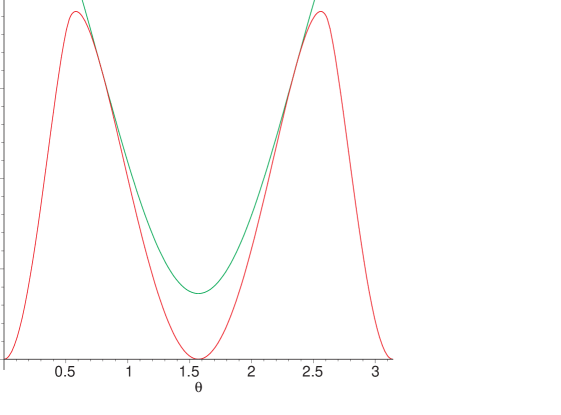
Figure 13: The red curve is $I(\theta)$ for the probability distribution $(0,\frac{1}{2},\frac{1}{2})$. The green curve is $\frac{1}{2}(1-H(\frac{1}{2}+\frac{\sqrt{3}}{4}))+\frac{1}{4}\cos 2\theta$. These curves are tangent at the points $\pi/4$ and $3\pi/4$, showing that the optimum measurement for accessible information is the von Neumann measurement with projectors $v_{\pi/4}$ and $v_{3\pi/4}$. It yields $1-H(\frac{1}{2}+\frac{\sqrt{3}}{4})$ bits of accessible information.

Appendix B: Convexity of accessible information on two pure states

For section 6, we needed a proof that the accessible information on two pure states $v_{1}$ and $v_{2}$ is a concave function in the probabilities of these pure states. As opposed to the rest of the paper, all logarithms in this section will have base e.

We first prove an inequality that will be used later. For $0\leq x<1$,

$$F(x)=\frac{2x}{1-x^{2}}-\log\left(\frac{1+x}{1-x}\right)\geq 0$$ (45)

It is easy to see that for $x=0$, both terms are 0. Differentiating and simplifying, we get

$$F^{\prime}(x)=\frac{4x^{2}}{(1-x^{2})^{2}}$$

which is positive for $0\leq x<1$, so $F(x)\geq 0$ in this range.

We now prove that the accessible information is a concave function in $p$ for an ensemble consisting of two pure states, $\left|\,v_{1}\right\rangle$ with probability $p$ and $\left|\,v_{2}\right\rangle$ with probability $1-p$. The formula for this accessible information is

$$I_{acc}=H(p)-H\left({\textstyle\frac{1}{2}+\frac{1}{2}\sqrt{1-4\kappa p(1-p)}}\right)$$

where $\kappa=|\langle v_{1}|v_{2}\rangle|^{2}$, and $H$ is the Shannon entropy function (which we will take to the base $e$ in this section). Proofs of this formula can be found in [10, 3, 12]. Substituting $q=p-1/2$, we get

$$I_{acc}=H\left({\textstyle\frac{1}{2}+q}\right)-H\left({\textstyle\frac{1}{2}+\frac{1}{2}\sqrt{1-\kappa(1-4q^{2})}}\right)$$ (46)

We wish to show that the second derivative of this quantity is negative with respect to $q$, for $-\frac{1}{2}<q<\frac{1}{2}$. Let

$$R=1-\kappa+4\kappa q^{2},$$

which is the quantity under the radical sign in Eq. (46).

We now differentiate $I_{acc}$ with respect to $q$ and obtain

$$\frac{d^{2}I_{acc}}{dq^{2}} = H^{\prime\prime}\left({\textstyle\frac{1}{2}+q}\right)-\frac{4q^{2}\kappa^{2}}{R}H^{\prime\prime}\left({\textstyle\frac{1}{2}+\frac{1}{2}\sqrt{R}}\right)-\frac{2\kappa(1-\kappa)}{R^{3/2}}H^{\prime}\left({\textstyle\frac{1}{2}+\frac{1}{2}\sqrt{R}}\right)$$

$$= -\frac{4}{1-4q^{2}}+\frac{4q^{2}\kappa^{2}}{R}\frac{4}{\kappa(1-4q^{2})}-\frac{2\kappa(1-\kappa)}{R^{3/2}}\ln\left(\frac{1-\sqrt{R}}{1+\sqrt{R}}\right)$$

$$= \frac{2(1-\kappa)}{(1-4q^{2})R^{3/2}}\left[-2R^{1/2}+\kappa(1-4q^{2})\ln\left(\frac{1+\sqrt{R}}{1-\sqrt{R}}\right)\right],$$

which quantity we wish to show is negative.

We thus need to show that

$$\kappa(1-4q^{2})\ln\left(\frac{1+\sqrt{R}}{1-\sqrt{R}}\right)\leq 2R^{1/2}$$

Since $\kappa(1-4q^{2})=1-R$, this is equivalent to

$$\log\left(\frac{1+\sqrt{R}}{1-\sqrt{R}}\right)\leq\frac{2\sqrt{R}}{1-R}.$$

However, this is the inequality (45) proven above, with $x=\sqrt{R}$, so we are done.

Appendix C: Accessible information for various $\alpha$.

In this section, we give graphs of the accessible information for various values of $\alpha$. These should be compared with Figure 14, which gives the graph for the planar trines, with $\alpha=0$. This illustrates the origin of the behavior of the two crossing curves giving the $C_{1,1}$ capacity in Figure 6. The line BZ gives the value of the local maximum at the central point $(\frac{1}{3},\frac{1}{3},\frac{1}{3})$, while the curve CY gives the behavior of the three at $(p,(1-p)/2,(1-p)/2)$. It appears from numerical experiments that this local maximum is achieved (or nearly achieved) using only three projectors for $\alpha\leq 0.27$. At a value of $\alpha$ slightly above $0.27$, the assumption that this local maximum is attained using a von Neumann measurement becomes false, and the curve of Figure 6, which appears to give a local maximum of the information attainable using von Neumann measurements, no longer corresponds to a local maximum of the accessible information. Note also that at the value $\alpha=0.27$, a POVM containing six projectors is required to achieve the $C_{1,1}$ capacity, even though there are only three 3-dimensional states in the ensemble.

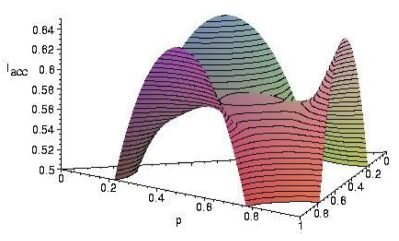
Figure 14: The accessible information for the planar trines. The probability distributions are represented by a triangle where the vertexes correspond to probability distributions $(1,0,0)$, $(0,1,0)$ and $(0,0,1)$. There are four local maxima, three at probability distributions symmetric with $(0,\frac{1}{2},\frac{1}{2})$, and one at $(\frac{1}{3},\frac{1}{3},\frac{1}{3})$. This was computed using a linear program, considering as possible POVM elements the projectors $(\cos\theta,\sin\theta)$, for 36,000 evenly spaced values of $\theta$. The linear programming package CPLEX was used to calculate the optimum for all probability distributions of the form $(\frac{a}{90},\frac{b}{90},\frac{c}{90})$, and this graph was drawn by interpolating from these values. We estimate the error for each of these points $(\frac{a}{90},\frac{b}{90},\frac{c}{90})$ to be less than $10^{-5}$.

here

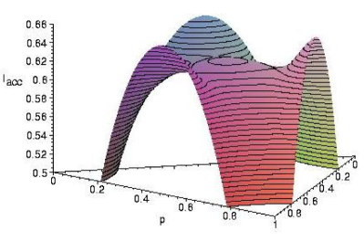
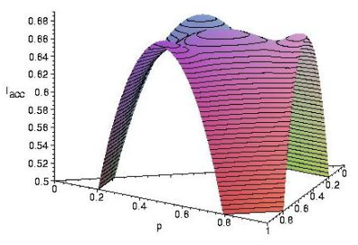
Figure 15: The accessible information for the trines with $\alpha=0.009$; as in Fig. 14, the probability distributions are represented by a triangle where the vertexes correspond to probability distributions $(1,0,0)$, $(0,1,0)$ and $(0,0,1)$. The maximum at $(0,0.5,0.5)$ (for the planar trines) has moved slightly away from the edge; the maximum value now occurs roughly at $(0.0012,0.4994,0.4994)$. The local maximum at $(\frac{1}{3},\frac{1}{3},\frac{1}{3})$ is growing larger with respect to the global maximum. This, and figures 16 and 17 were computed using the linear programming package CPLEX to determine the optimal measurement for points of the form $(\frac{a}{90},\frac{b}{90},\frac{c}{90})$, using projectors chosen from 96,000 vectors distributed around the unit sphere.

tb

Figure 16: The accessible information for the trines with $\alpha=0.018$; as in Fig. 14, the probability distributions are represented by a triangle where the vertexes correspond to probability distributions $(1,0,0)$, $(0,1,0)$ and $(0,0,1)$. Here, the three local maxima have moved farther in from the edges, and now occur at points symmetric with $(p,\frac{1-p}{2},\frac{1-p}{2})$ for $p\approx 0.027$; all four local maxima are now nearly equal in value.

tbh

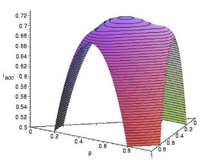
Figure 17: The accessible information for the trines with $\alpha=0.027$; as in Fig. 14, the probability distributions are represented by a triangle where the vertexes correspond to probability distributions $(1,0,0)$, $(0,1,0)$ and $(0,0,1)$. There are still four local maxima, where the ones on the shoulders occur at points symmetric with $(p,\frac{1-p}{2},\frac{1-p}{2})$ for $p\approx 0.105$; these will disappear before $\alpha$ reaches $0.0275$.

References

- [1] C. H. Bennett, D. P. DiVincenzo, C. A. Fuchs, T. Mor, E. Rains, P. W. Shor, J. A. Smolin, and W. K. Wootters, “Quantum nonlocality without entanglement,” Phys. Rev. A, vol. 59, pp. 1070–1091, 1999.
- [2] T. M. Cover and J. A. Thomas, Elements of Information Theory, Wiley, New York, 1991.
- [3] C. A. Fuchs Distinguishability and Accessible Information in Quantum Theory, Ph.D. Thesis, University of New Mexico, Albuquerque, NM, 1995.
- [4] C. A. Fuchs, personal communication.
- [5] C. A. Fuchs and C. M. Caves, “ Bounds for accessible information in quantum mechanics” Ann. N. Y. Acad. Sci., vol. 755, pp. 706–714, 1995
- [6] A. S. Holevo, “Information-theoretical aspects of quantum measurement,” Problemy Peredachi Informatsii vol. 9, no. 2, pp. 31–42 1973; English translation: A. S. Kholevo, Problems of Information Transmission, vol. 9, pp. 110-118, 1973.
- [7] A. S. Holevo, “Coding theorems for quantum channels,” Russian Math Surveys, vol. 53, pp. 1295–1331, 1998; LANL e-print quant-ph/9809023.
- [8] A. S. Holevo, “The capacity of quantum channel with general signal states,” IEEE Trans. Info Thy. 44, pp. 269–273 (1998).
- [9] M. Horodecki, P. Horodecki, and R. Horodecki, “Mixed-state entanglement and distillation: Is there a “bound” entanglement in nature?” Phys. Rev. Lett., vol. 80, pp. 5239–5242, 1998.
- [10] L. B. Levitin, “Physical information part II: Quantum systems,” in Workshop on Physics and Computation: PhysComp ’92 (D Matzke, ed.), IEEE Computer Society, Los Alamitos, CA, 1993, pp. 215–219.
- [11] L. B. Levitin, “Optimal quantum measurements for two pure and mixed states,” in Quantum Communications and Measurement (V. P. Belavkin, O. Hirota and R. L. Hudson, eds.), Plenum Press, New York, 1995, pp. 439–448.
- [12] M. Ban, M. Osaki, and O. Hirota, “Upper bound of the accessible information and lower bound of the Bayes cost in quantum signal detection processes” Phys. Rev. A, vol. 54, pp. 2718–27 1996.
- [13] A. Peres and W. K. Wootters, “Optimal detection of quantum information,” Phys. Rev. Lett., vol. 66, pp. 1119–1122 (1991).
- [14] M. Sasaki, S. M. Barnett, R. Jozsa, M. Osaki and O. Hirota, “Accessible information and optimal strategies for real symmetrical quantum sources,” Phys. Rev. A, vol. 59, 3325–3335, 1999, LANL e-print quant-ph/9812062.
- [15] B. Schumacher and M. D. Westmoreland, “Sending classical information via noisy quantum channels,” Phys. Rev. A 56, pp. 131–138 (1997).
- [16] C. E. Shannon, “A mathematical theory of communication,” The Bell System Tech. J., vol. 27, pp. 379–423, 623–656, 1948.
- [17] P. W. Shor, “The number of POVM elements needed for accessible information,” in Quantum Communication, Measurement, and Computing, Proceedings of the Fifth International Conference on Quantum Communication, Measurement and Computing, Capri, 1998, Kluwer Academic/Plenum Publishers, New York (2001) pp. 107-114.
- [18] J. A. Smolin, personal communication.