Local Detection of Entanglement

Abstract

We construct an explicit model where it can be established if a two mode pure Gaussian system is entangled or not by acting only on one of the parts that constitute the system. Measuring the dispersion in momentum and the time evolution of the dispersion in position of one particle we can tell if entanglement is present as well as the degree of entanglement of the system.

1 Introduction

One of the most intriguing features of Quantum Mechanics (QM) is entanglement and in the early times of QM it was recognized by Erwin Schrödinger schroedinger and by Einstein, Podolsky and Rosen epr . Later, John Bell bell showed that the non-local aspect of entanglement is experimentally testable through his famous inequality.

In recent years the interest in entanglement has increased considerably. First because it is a fundamental tool in Quantum Information Theory and a consistent characterization of its theoretical properties is needed. Second because the present stage of technology permits us to perform some experimental manipulations with it such as Quantum Teleportation bennett93 and Quantum Cryptography bennett92 ; eckert .

In the study of the properties of entanglement Peres peres and the Horodecki family h3 have derived a necessary and sufficient condition for the separability of $2\times 2$ and $2\times 3$ systems. Some years later Simon simon and Duan et al duan have obtained a necessary and sufficient condition for the separability of two-party Gaussian states. Given that the state is non-separable we should have a measure of the degree of this inseparability. There are at least three distinct measures of entanglement: the entanglement of formation bennettetal96c , the distillable entanglement bennettetal96a and the relative entropy of entanglement vedraletal97a ; vedraletal97b . In any calculations done with these three measures of entanglement and the two criteria for separability we must use the total density matrix of the bipartite system. That is, given the density matrix that describes the whole bipartite system we can determine if the system is separable or not and its degree of entanglement.

For pure states it is well known that the knowledge of the whole reduced density matrix allows us to decide whether or not the system is entangled. If the reduced density matrix is pure ($\text{Tr}(\rho_{1}^{2})=1$) the system is separable and entangled if it is not pure ($\text{Tr}(\rho_{1}^{2})<1$). This article aims to show that we need not know the whole reduced density matrix $\rho_{1}$ (or equivalently $\rho_{2}$) of a bipartite pure system to deduce if it is entangled or not. Here we show that only the diagonal elements of the reduced density matrix, even if it is written in a representation where it is not diagonal, are sufficient to detect entanglement.

To explicitly demonstrate this we construct two paradigmatic cases: a non-entangled two particle Gaussian wave function in configuration space and an entangled two particle Gaussian wave function. We then let both systems freely evolve in time. We show that when studying an individual particle of each case we get different results for the time evolution of the dispersion in position. This fact allows us to tell if we are working with a non-entangled or an entangled bipartite Gaussian wave function, and in the case of an entangled system we can also extract from this evolution the degree of entanglement.

Some aspects of this approach are similar to the total wave function reconstruction shown in Refs. leo ; richter ; ch . Here, however, we do not need to reconstruct the whole wave function describing the two particles. We only need two elements of the reduced wave function describing a single particle, i. e., its dispersion in position and in momentum. We should also mention that by employing the powerful techniques given in Refs. leo ; richter it might be possible to generalize the following approach to the case of mixed Gaussian states.

2 The non-entangled bipartite system

Consider a normalized one-dimensional separable two particle Gaussian wave function where we assume, with no loss of generality, that the two particles have the same mass $m$ but can in principle be distinguished from each other:

$$\psi(x_{1},x_{2},t)=\psi_{1}(x_{1},t)\otimes\psi_{2}(x_{2},t),$$ (1)

where

$$\psi_{1}(x_{1},t)=\int f(k_{1})e^{i[k_{1}x_{1}-\omega(k_{1})t]}dk_{1},$$ (2)

$$\psi_{2}(x_{2},t)=\int f(-k_{2})e^{i[k_{2}x_{2}-\omega(k_{2})t]}dk_{2}.$$ (3)

Here $\omega(k)=\frac{\hbar k^{2}}{2m}$ is the dispersion relation for a free particle and $f(k_{1})$, $f(-k_{2})$ represents the fact that we have Gaussian particles moving in opposite directions cohen :

$$f(k)=\frac{\sqrt{a}}{(2\pi)^{3/4}}e^{-\frac{a^{2}}{4}(k-k_{c})^{2}}.$$ (4)

In Eq. (4), $a$ represents the dispersion of the Gaussian wave packet centered in $k_{c}$ and the factor that multiplies the exponential is the normalization constant.

Integrating in $k_{1}$ and $k_{2}$, then multiplying $\psi(x_{1},x_{2},t)$ by its complex conjugate and finally integrating in $x_{2}$ we get the probability density of particle $1$ at time $t$ cohen :

$$|\varphi(x_{1},t)|^{2}=\sqrt{\frac{2}{\pi a^{2}}}\frac{1}{\sqrt{1+F(t)}}\exp\left[-\frac{2}{a^{2}}\frac{(x_{1}-v_{c}t)^{2}}{1+F(t)}\right],$$ (5)

where $F(t)$ and $v_{c}$ are given by:

$$F(t)=F(t,a)=\frac{4\hbar^{2}t^{2}}{m^{2}a^{4}}, v_{c}=\frac{\hbar k_{c}}{m}.$$ (6)

With Eq. (5) we can calculate the dispersion $\Delta x_{1}=\sqrt{\left<x_{1}^{2}\right>-\left<x_{1}\right>^{2}}$ of the position of particle $1$:

$$\Delta x_{1}(t)=\frac{a}{2}\sqrt{1+F(t)}.$$ (7)

We can also obtain the dispersion of the momentum of particle $1$ if we take the Fourier transform of Eq. (1). Then multiplying the result by its complex conjugate and integrating in $k_{2}$ we obtain:

$$|\tilde{\varphi}(k_{1},t)|^{2}=\sqrt{\frac{a^{2}}{2\pi}}\exp\left[-\frac{a^{2}}{2}(k_{1}-k_{c})^{2}\right].$$ (8)

Using Eq. (8) and the fact that $p_{1}=\hbar k_{1}$ we easily get:

$$\Delta p_{1}(t)=\frac{\hbar}{a}.$$ (9)

As expected for a free particle the dispersion in momentum is constant in time.

3 The entangled bipartite system

Let us now construct a normalized one-dimensional entangled two particle Gaussian wave function where we assume again, with no loss of generality, that the two particles have the same mass $m$ but can in principle be distinguished from each other.

$$\Psi(x_{1},x_{2},t=0) = \int dk_{1}dk_{2}f(k_{1},k_{2})$$ (10)

$$\times\psi_{1}(x_{1},0)\otimes\psi_{2}(x_{2},0).$$

Here $\psi_{1}(x_{1},0)$ and $\psi_{2}(x_{2},0)$ are given by:

$$\psi_{1}(x_{1},0)=e^{ik_{1}x_{1}}e^{\frac{-x_{1}^{2}}{a^{2}}},$$ (11)

$$\psi_{2}(x_{2},0)=e^{ik_{2}x_{2}}e^{\frac{-x_{2}^{2}}{a^{2}}}.$$ (12)

Eq. (10) is a superposition of bipartite Gaussian wave packets centered in $k_{1}$ and $k_{2}$ where $f(k_{1},k_{2})$ $=$ $g(k_{1},k_{2})$ $\delta(k_{1}+k_{2})$ are the expansion coefficients and $\delta(k_{1}+k_{2})$ is a restriction which entangles the system. This delta function can be viewed as the requirement for the conservation of momentum in the center of mass frame, that is, we superpose bipartite Gaussian wave packets where each party moves in opposite directions centered at the same momentum. Eqs. (11) and (12) are proportional to Eqs. (2) and (3) where we integrate for $t=0$ and substitute $k_{c}$ by $k_{1}$ and $k_{2}$ respectively. By using the delta function Eq. (10) can be rewritten as:

$$\Psi(x_{1},x_{2},0) = \int dk_{1}g(k_{1})$$ (13)

$$\times\left(e^{ik_{1}x_{1}}e^{\frac{-x_{1}^{2}}{a^{2}}}\right)\left(e^{-ik_{1}x_{2}}e^{\frac{-x_{2}^{2}}{a^{2}}}\right).$$

Eq. (13) clearly shows that $\delta(k_{1}+k_{2})$ entangles our system. Because $\Psi(x_{1},x_{2},0)$ cannot be written as a simple tensor product of a wave function belonging to particle $1$ and another belonging to particle $2$ we now deal with a non-separable wave function. Only if $g(k_{1})$ is another delta function we can disentangle the system and recover Eq. (1). In Eq. (13) $g(k_{1})$ is chosen to be a Gaussian distribution centered in $k_{c}$:

$$g(k_{1})=\sqrt{\frac{2}{\pi a^{2}}}f_{2}^{\frac{1}{4}}\frac{(b/2)}{\sqrt{\pi}}\exp\left[-(b/2)^{2}(k_{1}-k_{c})^{2}\right],$$ (14)

where $b$ is a new parameter that measures the degree of entanglement as explained below and $f_{n}=1+n\frac{a^{2}}{b^{2}}$, $n=1,2$. We can see that when $b\rightarrow\infty$ the function $\frac{(b/2)}{\sqrt{\pi}}\exp\left[-(b/2)^{2}(k_{1}-k_{c})^{2}\right]$ $\rightarrow$ $\delta(k_{1}-k_{c})$ arfken and $f_{2}\rightarrow 1$, showing that entanglement has disappeared. This can be seen doing a straightforward calculation using Eqs. (14) and (13):

$$\lim_{b\rightarrow\infty}\Psi(x_{1},x_{2},0) = \left[\left(\frac{2}{\pi a^{2}}\right)^{1/4}e^{ik_{c}x_{1}}e^{\frac{-x_{1}^{2}}{a^{2}}}\right]$$ (15)

$$\otimes \left[\left(\frac{2}{\pi a^{2}}\right)^{1/4}e^{-ik_{c}x_{2}}e^{\frac{-x_{2}^{2}}{a^{2}}}\right].$$

Eq. (15) is identical to Eq. (1) if we calculate the integrals in Eqs. (2) and (3). Furthermore, it can be shown that if $b\rightarrow 0$ and $a\rightarrow\infty$ Eq. (13) is the EPR state with $x_{0}=0$ englert . As stated in ref. englert , Eq. (13) can be viewed as a generalized version of the EPR wave function. These two facts suggest that $b$ should be considered as a measure of the degree of entanglement, where $b\rightarrow\infty$ represents no entanglement and $b\rightarrow 0$ represents the maximally entangled state.

Doing the integral in Eq. (13) we get the normalized bipartite Gaussian wave function at $t=0$:

$$\Psi(x_{1},x_{2},0) = \sqrt{\frac{2}{\pi a^{2}}}f_{2}^{\frac{1}{4}}e^{ik_{c}(x_{1}-x_{2})}$$ (16)

$$\times\exp\left[-\frac{f_{1}}{a^{2}}(x_{1}^{2}+x_{2}^{2})+\frac{2}{b^{2}}x_{1}x_{2}\right].$$

It is interesting to note that Eq. (16) represents a non-separable (entangled) state due to the term $\exp\left[\frac{2}{b^{2}}x_{1}x_{2}\right]$. If $b\rightarrow\infty$ this term tends to $1$ and we obtain Eq. (1) as a limiting case of Eq. (16). In other words, when $b\rightarrow\infty$ we have Eq. (1), a separable, non-entangled state, and for any other value of $b$ we have Eq. (16), a non-separable, entangled state.

In order to make rigorous that $b$ furnishes the degree of entanglement of the state given by Eq. (16) and that only when $b\rightarrow\infty$ we have a disentangled system we first calculate its correlation matrix (CM) and apply the Simon separability criterion simon , which shows that the bipartite Gaussian system is separable iff $b\rightarrow\infty$. After applying the Simon criterion, we make a local symplectic transformation in the CM to put it in its standard form simon ; duan and then calculate its entanglement of formation (EoF) werner , which is a monotonically decreasing function of the parameter $b$, proving that the higher $b$ the less entangled is the state. As we deal with a pure state, we note that we can calculate the von Neumann entropy of the reduced density matrix to obtain the entanglement of this system. However, we prefer using the EoF as given in Ref. werner since, in the particular case of symmetric bipartite Gaussian states, it is more straightforward than the usual procedure for pure states.

The CM completely specify a two mode Gaussian state and it is a $4\times 4$ matrix, which has the following elements simon ; duan :

$$\gamma_{ij}=\text{Tr}\left[(R_{i}R_{j}+R_{j}R_{i})\rho\right]-2\text{Tr}[R_{i}\rho]\text{Tr}[R_{j}\rho],$$ (17)

where $R=(X_{1},P_{1},X_{2},P_{2})^{T}$ and $R_{j}$ are the position and momentum operators of the two particles. Doing the calculations we get the following CM:

$$\gamma=\left(\begin{array}[]{cc}A&C\\ C^{T}&A\end{array}\right),$$ (18)

where

$$\begin{array}[]{ccc}A=\left(\begin{array}[]{cc}\frac{a^{2}f_{1}}{2f_{2}}&0\\ 0&\frac{2\hbar^{2}f_{1}}{a^{2}}\end{array}\right),&C=\left(\begin{array}[]{cc}\frac{a^{4}}{2b^{2}f_{2}}&0\\ 0&-\frac{2\hbar^{2}}{b^{2}}\end{array}\right).\end{array}$$ (19)

The Simon separability criterion says that the above CM represents a non-entangled system iff nota1 :

$$I = \text{det}A\text{det}B+\left(\hbar^{2}-\left|\text{det}C\right|\right)^{2}-\text{Tr}\{AJCJBJC^{T}J\}$$ (20)

$$-\hbar^{2}(\text{det}A+\text{det}B)\geq 0,$$

where $J=\left(\begin{array}[]{cc}0&1\\ -1&0\end{array}\right)$. But a simple calculation shows that the rhs of Eq. (20) is:

$$I=-4\hbar^{4}\frac{a^{4}}{b^{4}}\frac{1}{f_{2}}.$$ (21)

Hence, $I<0$ except when $b\rightarrow\infty$, proving that for any other value of $b$ we have an entangled state.

We now make the following local symplectic transformation $S$ $=$ diag $(s,$ $s^{-1},$ $s,$ $s^{-1})$, where $s$ $=$ $\left(4\hbar^{2}f_{2}/a^{4}\right)^{1/4}$. This brings $\gamma$ to its standard form $\gamma_{0}=S\gamma S^{T}$ simon ; duan :

$$\gamma_{0}=\left(\begin{array}[]{cccc}n&0&k_{x}&0\\ 0&n&0&-k_{p}\\ k_{x}&0&n&0\\ 0&-k_{p}&0&n\end{array}\right),$$ (22)

where $n=\hbar f_{1}/\sqrt{f_{2}}$ and $k_{x}=k_{p}=\hbar a^{2}/(b^{2}\sqrt{f_{2}})$. This is a symmetric Gaussian system and Giedke et al. werner have shown that the EoF for this state is:

$$EoF(\Psi)=f\left[\sqrt{(n-k_{x})(n-k_{p})}\right],$$ (23)

where,

$$f(\delta)=c_{+}(\delta)\,\log_{2}[c_{+}(\delta)]-c_{-}(\delta)\,\log_{2}[c_{-}(\delta)].$$ (24)

Here $c_{\pm}(\delta)=(\delta^{-1/2}\pm\delta^{1/2})^{2}/4$. Analyzing the behavior of the EoF given by Eq. (23) we clearly see that it is a decreasing function of the parameter $b$ (Figs. 1 and 2).

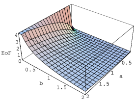
Figure 1: Entanglement of formation, Eq. (23), for the symmetric Gaussian state given by Eq. (16), as function of the parameters $a$ and $b$, where we have put $\hbar=1$. We clearly see the EoF increasing as $b\rightarrow 0$ and decreasing as $a\rightarrow 0$.

Figure 2: Entanglement of formation, Eq. (23), as a function of $1/b$ for ten values of the parameter $a$. From bottom to top the parameter $a$ varies from $1$ to $10$ in increments of one unit. We have set $\hbar=1$. We clearly see that the EoF increases as $b$ decreases and that for a given b, the higher $a$, the greater the EoF.

Working in the Heisenberg picture we easily obtain for a free evolution,

$$\Delta x_{1}(t)=\frac{a}{2}\sqrt{\frac{f_{1}}{f_{2}}[1+f_{2}F(t)]},$$ (25)

$$\Delta p_{1}(t)=\frac{\hbar}{a}\sqrt{f_{1}}.$$ (26)

Again, due to the free evolution of particle $1$ the dispersion in momentum does not vary in time.

We should mention that the formal solution of the Heisenberg equations of motion for the observables $x_{1}(t)$, $x_{1}^{2}(t)$, $p_{1}(t)$, and $p_{1}^{2}(t)$ are identical for the entangled and non-entangled case. Only when we take the mean values $\langle x_{1}(t)\rangle$, $\langle x_{1}^{2}(t)\rangle$, $\langle p_{1}(t)\rangle$, and $\langle p_{1}^{2}(t)\rangle$ we obtain different quantities. This is due to the fact that we have different initial wave functions. In other words, entanglement manifests itself furnishing different initial conditions for the Heisenberg equations of motion, which imply different evolutions for the dispersions.

4 The measuring protocol

As we have all tools now, that is, all the dispersions in position and in momentum for the entangled and non-entangled case, we develop a measurement procedure to be used in an ensemble of two particle Gaussian systems which allows us to locally decide whether or not the particles are entangled. From now on we assume $\hbar=m=1$ for simplicity.

Let Bob be our physicist who receives one of the particles of the bipartite Gaussian system produced by Alice. Bob knows, because Alice has told him, that all the particles he receives are either entangled or non-entangled Gaussian wave packets, according to the two constructions explained above. There are no other possibilities. Alice produces many pairs at once. And continues to produce many pairs at once for different times. Of course Bob does not know the values of the parameters $a$ and $b$ used by Alice. But Bob is curious enough and wants to know whether his particles are entangled or not. Bob cannot use any further classical communication, he can act only locally on his particles and he is able only to measure the dispersions in position and in momentum of his particles, that is, the diagonal elements of the system reduced density matrix. He proceeds as follows:

First he measures, using a sub-ensemble, the dispersion in momentum of his wave packets. He obtains $\Delta p_{1}=u$. He does not know yet whether Eq. (9) or Eq. (26) represents what he measures. However he knows that it must be one of these two possibilities, which imply only two possible time evolution for the dispersion in the position of his particles.

If his particles are not entangled and Bob uses in Eq. (7) the fact that $\Delta p_{1}(t)=u=\frac{1}{a}$ he gets:

$$\Delta x_{1}(t)=\frac{1}{2u}\sqrt{1+4u^{4}t^{2}}.$$ (27)

But if Bob’s particles are entangled and now he uses the fact that $\Delta p_{1}(t)=u=\frac{\sqrt{f_{1}}}{a}$, Eq. (25) becomes:

$$\Delta x_{1}(t)=\frac{1}{2u}\sqrt{\frac{u^{4}b^{4}}{u^{4}b^{4}-1}+4u^{4}t^{2}}.$$ (28)

Looking at Eqs. (27) and (28) we see that if Bob knows at what time Alice has begun to produce the pairs he is able to discover, with only one measurement of $\Delta x_{1}$, whether his particles are entangled with Alice’s or not. The reason for this is simple: Let us suppose, with no loss of generality, that Alice begins to produce the pairs of particles at $t=0$. Measuring the dispersion in position for a given time $t$ Bob obtains $\Delta x_{1}(t)$. Remembering that Bob also knows the value of $u$, he can calculate, using Eq. (27), the value of $\Delta x_{1}(t)$. If this calculated value of the dispersion agrees with the measured one, Bob has the non-entangled case. If these values of $\Delta x_{1}$ are different, Bob has entanglement. In this last case, using Eq. (28) Bob can obtain the parameter $b$. For any $t$ Bob can use this procedure. Bob sees two distinct curves for the time evolution of $\Delta x_{1}(t)$, whether his particles are entangled or not. See Fig. $1$ below:

Figure 3: The dashed curve is the time evolution of the dispersion in position for an entangled Gaussian wave packet while the solid curve represents the non-entangled case. We have chosen $b=1$ and $u=1.01$.

Analyzing Eq. (28) we see that for it to be valid for all $t\geq 0$ we must have for the entangled case:

$$ub>1.$$ (29)

It is worth noting that asymptotically Eq. (27) and (28) are the same. Therefore, in order for Bob to correctly distinguish between the two cases he should make his measurements for times smaller than a critical time $t_{c}$, which is defined to be the time where the time independent term inside the square root of Eq. (28) is of the order of the $t^{2}$ term:

$$t_{c}\approx\frac{b^{2}}{2\sqrt{u^{4}b^{4}-1}}.$$ (30)

We can increase $t_{c}$ making $ub\rightarrow 1$. This might seem as a limitation of our procedure but as Alice sends a classical message to Bob defining the origin of time, Bob can start making measurements as early as possible.

Now let us make things harder to Bob. We assume from now on that Bob does not know when and where Alice has begun to produce the pairs. This fact means that Bob cannot use the previous procedure to answer whether or not his particles are entangled with Alice’s. The previous protocol fails because Bob does not know what time $t$ he should use to calculate $\Delta x_{1}(t)$, which would have allowed him to compare this calculated value with the measured $\Delta x_{1}(t)$.

We first prove why a single measurement at time $t$ is not enough for Bob to tell whether his particles are entangled or not. We are now assuming that he does not know when Alice has begun to produce the particles. The proof is achieved showing that the diagonal elements of the reduced density matrix (in position and in momentum representation) of the non-entangled system can be made identical to the diagonal elements of the reduced density matrix of the entangled system for $t=0$. (The same reasoning applies to any $t$, but for $t=0$ the calculations are much simpler and we do not lose in generality).

For $t=0$ the diagonal elements of the reduced density matrix of the entangled system in momentum representation is

$$\varrho_{1}(k_{1}) = \int\left<k_{1},k_{2}\right|\Psi\left>\right<\Psi\left|k_{1},k_{2}\right>dk_{2}$$ (31)

$$= \sqrt{\frac{a^{2}}{2\pi f_{1}}}\exp\left[-\frac{a^{2}}{2f_{1}}(k_{1}-k_{c})^{2}\right].$$

For any $t$, the diagonal elements of the reduced density matrix of the non-entangled system in the momentum representation, according to Eq. (8), reads:

$$\rho_{1}(k_{1},t) = \int\left<k_{1},k_{2}\right|\psi\left>\right<\psi\left|k_{1},k_{2}\right>dk_{2}$$ (32)

$$= \sqrt{\frac{a^{\prime 2}}{2\pi}}\exp\left[-\frac{a^{\prime 2}}{2}(k_{1}-k_{c})^{2}\right].$$

If we want identical diagonal elements of the reduced density matrices we must impose that:

$$a^{\prime}=\frac{a}{\sqrt{f_{1}}}=\frac{1}{u}.$$ (33)

The diagonal elements of the reduced density matrix for $t=0$ of the entangled system written in the position representation is:

$$\varrho_{1}(x_{1}) = \int\left<x_{1},x_{2}\right|\Psi\left>\right<\Psi\left|x_{1},x_{2}\right>dx_{2}$$ (34)

$$= \sqrt{\frac{2f_{2}}{\pi a^{2}f_{1}}}\exp\left[-\frac{2f_{2}}{a^{2}f_{1}}x_{1}^{2}\right].$$

As stated in Eq. (5), the diagonal elements of the reduced density matrix for any $t$ of the non-entangled system in position representation is:

$$\rho_{1}(x_{1}) = \int\left<x_{1},x_{2}\right|\psi\left>\right<\psi\left|x_{1},x_{2}\right>dx_{2}$$ (35)

$$= \sqrt{\frac{2}{\pi a^{\prime 2}}}\frac{1}{\sqrt{1+F(t,a^{\prime})}}$$

$$\times\exp\left[-\frac{2}{a^{\prime 2}}\frac{(x_{1}-v_{c}t)^{2}}{1+F(t,a^{\prime})}\right].$$

If we want Eqs. (34) and (35) giving the same statistical predictions we must have:

$$\frac{2f_{2}}{a^{2}f_{1}}=\frac{2}{a^{\prime 2}}\frac{1}{1+F(t,a^{\prime})}.$$ (36)

Eq. (36) is a restriction which forces the two density matrix to give the same dispersion in position. (We do not need to bother with the first order moment of these Gaussian functions because a translation of the $x_{1}$-axis sets it to zero.) If we use Eqs. (33) and (36) and the fact that $f_{n}=1+n\frac{a^{2}}{b^{2}}$ we arrive at the following condition:

$$t=\frac{1}{2u^{2}}\frac{1}{\sqrt{u^{4}b^{4}-1}}$$ (37)

Eq. (37) says that for only, and only one time $t$, the diagonal elements of the reduced density matrices, one obtained from the entangled system and the other one obtained from the non-entangled system, furnish the same statistical predictions. This implies that single measurements of the dispersion in momentum and in position of particle $1$ do not tell us unequivocally whether we are dealing with a non-entangled or entangled Gaussian bipartite system. (Unless, of course, we know when Alice has begun to produce the pairs.) See Fig. 4.

Figure 4: The dashed curve is the time evolution of the dispersion in position for an entangled Gaussian wave packet produced $1$ unity of time after the production of the non-entangled case, which is represented by the solid curve. The curves intercept each other for $t\approx 2.46$. If Bob measures $\Delta x_{1}$ for this time, he cannot distinguish between the two ways in which Alice can produce the pairs of particles. For any other point of the dashed curve we can find a solid one that crosses it. Therefore, Bob cannot distinguish how his particles were produced if he measures $\Delta x_{1}$ only once. Here we have chosen $b=1$ and $u=1.01$.

To circumvent the limitation of the previous protocol Bob may apply the following one, which explicitly uses the difference in time evolution of the two systems:

Bob again initially measures the dispersion in momentum of his particles ($\Delta p_{1}=u$). As he does not know when and where Alice begins to produce the pairs of Gaussian particles, the time evolution of the dispersions in position for the non-entangled and entangled systems are:

$$\Delta x_{1}(t)=\frac{1}{2u}\sqrt{1+4u^{4}(t+t_{0})^{2}}.$$ (38)

$$\Delta x_{1}(t)=\frac{1}{2u}\sqrt{\frac{u^{4}b^{4}}{u^{4}b^{4}-1}+4u^{4}(t+t_{0})^{2}}.$$ (39)

Here $t_{0}$ is the time elapsed from the production of the pair by Alice until Bob makes his first set of measurements. Bob now makes several measurements of the dispersion in position for different times $t$. With these measurements he obtains the following set of points:

$$\{(\Delta x_{1}(0),0),(\Delta x_{1}(t_{1}),t_{1}),\ldots,(\Delta x_{1}(t_{n}),t_{n})\}.$$

He makes as many measurements as possible. With the $n$ pairs of points above he fits the following curve, where $\alpha$ and $\beta$ are the free parameters and $u$ is already known:

$$\Delta x_{1}(t)=\frac{1}{2u}\sqrt{\alpha+4u^{4}(t+\beta)^{2}}.$$ (40)

Looking at Eqs. (40), (38), and (39) we see that if the parameter $\alpha=1$ Bob is dealing with non-entangled Gaussian functions, but if $\alpha\neq 1$ Bob deals with entangled particles. And using $\alpha$ Bob can calculate the value of the degree of entanglement $b$. Just for completeness we mention that $\beta$ furnishes the time $t_{0}$. For this protocol to be optimal, Bob should begin his measurements as soon as possible since, asymptotically in time, Eqs. (38) and (39) are seen to become identical.

5 Conclusion

We have shown an explicit model using two particle Gaussian systems where we can decide if we are dealing with non-entangled or entangled pairs acting only on one of the particles and measuring only the diagonal elements of its reduced density matrix. Measuring the dispersion in momentum and then the time evolution of the dispersion in position of one member of the pair it is possible to discern between the entangled and non-entangled cases. It is also possible with this procedure to determine the degree of the entanglement of the system. The above model suggests that just one part of the whole system can furnish more information about the degree of the entanglement of the system than we had imagined.

Finally it is important to note that the presented measurement protocol uses the time evolution of the diagonal elements of the reduced density matrix to determine whether or not we have entanglement. This fact shows that we may have a new tool to analyze the properties of entangled systems, i. e., the dynamical evolution of entangled states. So far all the methods used to study the properties of entangled systems have not employed the dynamics of the system. We are hopeful that studying the dynamics of entangled systems will help us to deepen our understanding of entanglement and possibly it will unravel new features of entanglement not yet explored.

References

- (1) E. Schrödinger, Proc. Camb. Phil. Soc. 31, 555 (1935).
- (2) A. Einstein, B. Podolsky, and N. Rosen, Phys. Rev. 47, 777 (1935).
- (3) J. S. Bell, Physics 1, 195 (1964).
- (4) C. H. Bennett, G. Brassard, C. Crépeau, R. Jozsa, A. Peres, and W. K. Wootters, Phys. Rev. Lett. 70, 1895 (1993).
- (5) C. H. Bennett, G. Brassard, and N. D. Mermin, Phys. Rev. Lett. 68, 557 (1992).
- (6) A. K. Ekert, Phys. Rev. Lett. 67, 661 (1991).
- (7) A. Peres, Phys. Rev. Lett. 77, 1413 (1996).
- (8) M. Horodecki, P. Horodecki, and R. Horodecki, Phys. Lett. A 223, 1 (1996).
- (9) R. Simon, Phys. Rev. Lett. 84, 2726 (2000).
- (10) L-M. Duan, G. Giedke, J. I. Cirac, and P. Zoller, Phys. Rev. Lett. 84, 2722 (2000).
- (11) To recover the Simon separability criterion as it was presented in Simon’s paper simon we should substitute in Eq. (20) by . This difference is due to the fact that Simon’s CM is defined as the half of our CM . We use the same notation as duan .
- (12) C. H. Bennett, D. P. DiVincenzo, J. A. Smolin, and W. K. Wootters, Phys. Rev. A 54, 3824 (1996).
- (13) C. H. Bennett, G. Brassard, S. Popescu, B. Schumacher, J. A. Smolin, and W. K. Wootters, Phys. Rev. Lett. 76, 722 (1996).
- (14) V. Vedral, M. B. Plenio, M. A. Rippin, and P. L. Knight, Phys. Rev. Lett. 78, 2275 (1997).
- (15) V. Vedral, M. B. Plenio, K. Jacobs, and P. L. Knight, Phys. Rev. A 56, 4452 (1997).
- (16) U. Leonhardt and M. G. Raymer, Phys. Rev. Lett. 76, 1985 (1996).
- (17) T. Richter and A. Wünsche, Phys. Rev. A 53, R1974 (1996).
- (18) Ch. Kurtsiefer, T. Pfau, and J. Mlynek, Nature 386, 150 (1997).
- (19) C. Cohen-Tannoudji, B. Diu, and F. Laloë, Quantum Mechanics, Vol. 2 (Hermann and John Wiley & Sons, Paris, 1977), Chap. 1, Complement .
- (20) G. Arfken, Mathematical Methods for Physicists, (Academic Press, Orlando, 1985), Chap 8.
- (21) B-G. Englert and K. Wódkiewicz, P hys. Rev. A 65, 054303 (2002).
- (22) G. Giedke, M. M. Wolf, O. Krüger, R. F. Werner, and J. I. Cirac, Phys. Rev. Lett. 91, 107901 (2003).