Two-photon linewidth of light “stopping” via electromagnetically induced transparency

Abstract

We analyze the two-photon linewidth of the recently proposed adiabatic transfer technique for “stopping” of light using electromagnetically induced transparency (EIT). We show that a successful and reliable transfer of excitation from light to atoms and back can be achieved if the spectrum of the input probe pulse lies within the initial transparency window of EIT, and the two-photon detuning $\delta$ is less than the collective coupling strength (collective vacuum Rabi-frequency) $g\sqrt{N}$ divided by $\sqrt{\gamma T}$, with $\gamma$ being the radiative decay rate, $N$ the effective number of atoms in the sample, and $T$ the pulse duration. Hence in an optically thick medium light “storage” and retrieval is possible with high fidelity even for systems with rather large two-photon detuning or inhomogeneous broadening.

I Introduction

One of the challenges of practical quantum information processing and communication is the faithful storage and retrieval of an unknown quantum state in a memory system [1]. Recently we have proposed a technique for a controlled transfer of the quantum state of a photon wavepacket to and from a collective atomic spin excitation [2, 3, 4] using electromagnetically induced transparency (EIT) [5] and Raman adiabatic passage [6]. When a weak probe pulse and a much stronger control field couple two metastable states of a 3-level atom through a Raman transition in two-photon (but not necessarily in single-photon) resonance, the control field renders an otherwise optically thick medium transparent. The induced transparency is associated with a substantial reduction of the propagation velocity of the probe pulse due to the formation of a coupled field-spin excitation called dark-state polariton [3, 4]. Dynamically reducing the intensity of the control field decelerates the polariton and can bring it to a full stop [7, 8]. When the velocity reaches zero, the polariton is entirely matter like and the quantum state of the original light pulse is completely transferred to a collective spin excitation of the atomic ensemble. The process is reversible and the quantum state can be transferred back to a light pulse by re-accelerating the polariton, which can be an exact replica of the original one or — if desired — can occupy different modes (different direction, carrier frequency etc.) [9, 10].

Essential for a high fidelity of the transfer process is an explicitly time-dependent control field which varies in most parts adiabatically. When the group velocity of the polariton approaches zero, so does the spectral width of transparency in EIT. Adiabatic following leads however to a narrowing of the spectral width of the probe pulse parallel to the narrowing of the transparency window and thus there are no absorption losses during the slow-down provided the carrier frequency of the probe pulse and the control field are in precise two-photon resonance [4]. For a non-vanishing two-photon detuning the pulse spectrum will move outside the transparency region at some finite value of the group velocity. Thus the question arises what values of the two-photon detuning, if any, are tolerable to maintain a sufficiently high fidelity of the quantum memory. This question is of particular practical importance in gas experiments with different pump and probe frequencies [7, 8] or different propagation directions of the fields since two-photon Doppler-shifts are then no longer negligible. An estimate of the two-photon linewidth of light “storage” is furthermore interesting for applications in rare-earth doped solid-state materials with inhomogeneously broadened two-photon transitions [11].

In the present paper we analyze the two-photon linewidth of the storage process based on an analytic perturbation theory and compare it with exact numerical results. We will show that under otherwise favorable conditions, the linewidth is given by the collectively enhanced coupling strength (vacuum Rabi-frequency) $g\sqrt{N}$, with $N$ being the number of atoms divided by $\sqrt{\gamma T}$, with $\gamma$ being the excited-state decay rate and $T$ the characteristic pulse duration. In an optically thick ensemble this quantity can be large and thus rather large two-photon detunings are tolerable.

II model

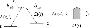
We consider the quasi 1-dimensional system shown in Fig. 1. A probe pulse with positive frequency part of the electric field $E^{(+)}$ couples the transition between the ground state $|b\rangle$ and the excited state $|a\rangle$. $\delta_{ab}=\omega_{ab}-\nu$ is the detuning between the carrier frequency $\nu$ and the atomic transition frequency $\omega_{ab}$. The upper level $|a\rangle$ is coupled to the stable state $|c\rangle$ via a coherent control field with Rabi-frequency $\Omega$. $\delta_{ac}=\omega_{ac}-\nu_{c}$ is the corresponding detuning of the coupling transition. The Rabi-frequency of the coupling field is assumed to be large compared to that of the probe pulse and undepleted. Furthermore we assume that $\Omega$ is only a function of time. This can be realized either by perpendicular incidence of the control field or, in the case of co-propagating fields, if the group velocity of the probe pulse is at all times much less than that of the coupling field. In the latter case retardation effects of the control field can be disregarded.

FIG. 1.: 3-level $\Lambda$-type medium coupled to a control field with Rabi-frequency $\Omega(t)$ and a probe field $E(z,t)$.

Within the rotating wave approximation the interaction between the atoms and the fields can be described by density matrix equations in a rotating frame

$$\dot{\rho}_{aa} = -\gamma_{a}{\rho}_{aa}-ig\Bigl{(}{\cal E}^{*}{\rho}_{ab}-c.c.\Bigr{)}$$ (2)

$$-i\Bigl{(}\Omega^{*}{\rm e}^{-ikz}{\rho}_{ca}-c.c.\Bigr{)},$$

$$\dot{\rho}_{bb} = \gamma_{a\to b}{\rho}_{aa}+ig\Bigl{(}{\cal E}^{*}{\rho}_{ab}-c.c.\Bigr{)},$$ (3)

$$\dot{\rho}_{cc} = \gamma_{a\to c}{\rho}_{aa}+i\Bigl{(}\Omega^{*}{\rm e}^{-ikz}{\rho}_{ac}-c.c.\Bigr{)},$$ (4)

$$\dot{\rho}_{ab} = -\Bigl{(}\gamma_{ab}+i\delta_{ab}\Bigr{)}{\rho}_{ab}+ig{\cal E}\Bigl{(}{\rho}_{bb}-{\rho}_{aa}\Bigr{)}$$ (6)

$$+i\Omega{\rm e}^{ikz}{\rho}_{cb},$$

$$\dot{\rho}_{ac} = -\Bigl{(}\gamma_{ac}+i\delta_{ac}\Bigr{)}{\rho}_{ac}+i\Omega{\rm e}^{ikz}\Bigl{(}{\rho}_{cc}-{\rho}_{aa}\Bigr{)}$$ (8)

$$+ig{\cal E}{\rho}_{bc},$$

$$\dot{\rho}_{cb} = -i\Bigl{(}\delta_{ab}-\delta_{ac}\Bigr{)}\rho_{cb}+i\Omega^{*}{\rm e}^{-i\Delta kz}{\rho}_{ab}-ig{\cal E}{\rho}_{ca},$$ (9)

where $\gamma_{a}=\gamma_{a\to b}+\gamma_{a\to c}$ and $\gamma_{a\to b},\gamma_{a\to c}$ denote longitudinal and $\gamma_{\mu\nu}$ transverse decay rates, and $k=\nu/c$ is the wavenumber of the probe field propagating in the $z$ direction. We have also introduced the dimensionless slowly varying field amplitude

$$E^{(+)}(z,t)=\sqrt{\frac{\hbar\nu}{2\varepsilon_{0}V}}\,{\cal E}(z,t)\,{\rm e}^{i\frac{\nu}{c}(z-ct)},$$ (10)

with $V$ being the interaction volume. To simplify the following analytic discussion it is useful to consider a resonant probe field, i.e. to assume $\delta_{ab}=0$, while keeping $\delta_{ac}\neq 0$.

The evolution of the probe pulse can be described in slowly varying amplitude approximation (SVEA) by the propagation equation

$$\left(\frac{\partial}{\partial t}+c\frac{\partial}{\partial z}\right){\cal E}(z,t)={i}gN\,\rho_{ab}(z,t).$$ (11)

Here $g=\wp\sqrt{\frac{\nu}{2\hbar\epsilon_{0}V}}$ is the atom-field coupling constant proportional to the dipole moment $\wp$ of the probe transition.

It was shown in Ref.[3, 4] that the propagation of elm. pulses in an EIT medium can be be most easily understood in terms of polariton-like fields, which are superpositions of the (dimensionless) electric field amplitude ${\cal E}$ and the spin coherence $\rho_{cb}$ between the two lower levels. There are two types of polaritons called dark-state ($\Psi$) and bright-state ($\Phi$) polaritons:

$$\Psi(z,t) = \cos\theta(t){\cal E}(z,t)-\sin\theta(t)\sqrt{N}\rho_{cb}\,{\rm e}^{ikz},$$ (12)

$$\Phi(z,t) = \sin\theta(t){\cal E}(z,t)+\cos\theta(t)\sqrt{N}\rho_{cb}\,{\rm e}^{ikz},$$ (13)

The mixing angle $\theta$ in eq.(12) and (13) is defined via $\tan\theta(t)=g\sqrt{N}/\Omega(t)$, where we have assumed without loss of generality a real Rabi-frequency of the drive field $\Omega=\Omega^{*}$.

One can transform the equations of motion for the electric field and the atomic variables into the polariton variables. In the approximation of low probe field intensities — which is most interesting for quantum memory purposes — one finds

$$\biggl{[}\frac{\partial}{\partial t}+c\cos^{2}\theta\frac{\partial}{\partial z}-i\,\delta\sin^{2}\theta\biggr{]}\,\Psi=$$ (14)

$$\qquad-\left[\dot{\theta}+\sin\theta\cos\theta\,\left(c\frac{\partial}{\partial z}+i\,\delta\right)\right]\Phi,$$ (15)

and

$$\Phi=\frac{\sin\theta}{g^{2}N}\times$$ (16)

$$\quad\times\biggl{(}\frac{\partial}{\partial t}+\gamma\Bigr{)}\biggl{[}\tan\theta\left(\frac{\partial}{\partial t}-i\delta\right)\biggr{]}\Bigl{(}\sin\theta\,\Psi-\cos\theta\,\Phi\Bigr{)},$$ (17)

with $\gamma=\gamma_{ab}$. One here has to keep in mind that the mixing angle $\theta$ is a function of time.

III polariton dynamics for finite two-photon detuning

In order to find approximate analytic solutions of these equations we introduce a characteristic time $T$ of the transfer and a corresponding dimensionless time, length and detuning. We can then identify two expansion parameter, $\epsilon_{1}=(g\sqrt{N}T)^{-1}$, defining an adiabatic expansion, and $\epsilon_{2}=\delta/(g\sqrt{N})$ characterizing the magnitude of the two-photon detuning. Furthermore we assume for simplicity that $T$ is much larger than the decay time, i.e. $\gamma T\gg 1$, which is usually well satisfied for conditions of light “stopping”.

In the adiabatic limit, i.e. up to first order of $\epsilon_{1}$, and for small detuning, i.e. in first order of $\epsilon_{2}$ one finds:

$$\biggl{(}\frac{\partial}{\partial t}+c\cos^{2}\theta\frac{\partial}{\partial z}-i\delta\sin^{2}\theta(t)\biggr{)}\,\Psi^{(0)}(z,t) = 0,$$ (18)

$$\Phi^{(0)}(z,t) = 0.$$ (19)

In this limit the bright-state polariton is not exited. The dark-state polariton propagates with a form-stable envelope and with instantaneous velocity $v_{\rm gr}(t)=c\cos^{2}\theta(t)$. The small two-photon detuning simply causes a time dependent phase shift (chirp) of the pulse:

$$\Psi^{(0)}(z,t) = \Psi\Bigl{(}z-c\int_{0}^{t}\!\!{\rm d}t^{\prime}\cos^{2}\theta(t^{\prime}),0\Bigr{)}$$ (21)

$$\times\exp\left\{i\delta\int_{0}^{t}\!\!{\rm d}t^{\prime}\sin^{2}\theta(t^{\prime})\right\}$$

In next order of perturbation in $\epsilon_{1}$ and $\epsilon_{2}$ a longer calculation gives a finite excitation of the bright-state polariton due to non-adiabatic couplings and the non-vanishing two-photon detuning

$$\Phi^{(2)} = \frac{\gamma\sin^{2}\theta}{g^{2}N}\Biggl{[}\dot{\theta}-i\delta\sin\theta\cos\theta\Biggr{]}\Psi^{(2)}$$ (23)

$$-\frac{\gamma\sin^{3}\theta\cos\theta}{g^{2}N}c\frac{\partial}{\partial z}\Psi^{(2)}.$$

Here we made use of the fact that in the same order of approximation $\partial\Psi/\partial t$ can be replaced by $i\delta\sin^{2}\theta\Psi-c^{2}\cos^{2}\theta(\partial\Psi/\partial z)$. Substituting this result into the right hand side of eq.(15) gives the equation of motion

$$\biggl{(}\frac{\partial}{\partial t}+c\cos^{2}\theta\frac{\partial}{\partial z}-i\delta\sin^{2}\theta(t)\biggr{)}\Psi^{(2)}=$$ (24)

$$\quad-\biggl{(}A_{0}(t)+\delta^{2}A_{1}(t)\biggr{)}\Psi^{(2)}-i\delta B_{0}(t)c\frac{\partial}{\partial z}\Psi^{(2)}$$ (25)

$$\quad-C_{0}(t)\,c^{2}\frac{\partial^{2}}{\partial z^{2}}\Psi^{(2)}$$ (26)

with

$$A_{0}(t) = \frac{\gamma}{g^{2}N}\dot{\theta}^{2}\sin^{2}\theta,$$ (27)

$$A_{1}(t) = \frac{\gamma}{g^{2}N}\sin^{4}\theta\cos^{2}\theta,$$ (28)

$$B_{0}(t) = -\frac{2\gamma}{g^{2}N}\sin^{4}\theta\cos^{2}\theta,$$ (29)

$$C_{0}(t) = -\frac{\gamma}{g^{2}N}\sin^{4}\theta\cos^{2}\theta,$$ (30)

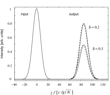
Since all coefficients $A_{0},\dots,C_{0}$ depend only on time, eq.(25) can easily be integrated by Fourier-transformation in space. To illustrate the accuracy of the approximations we have compared in Fig.2 the analytical expression for the polariton intensity obtained from (25) after storage and release with an exact numerical result. One recognizes rather good agreement even for values of $\epsilon_{2}$ as large as $0.5$.

$A_{0}$ is a dissipative loss term due to non-adiabatic couplings which restricts the speed of rotation between field-like and matter-like behavior of the polariton [4]. $C_{0}$ causes dissipative losses of the high-frequency components of the polariton. It restricts the spectral width of the light pulse to within the initial transparency window of EIT (see [4] for details).

FIG. 2.: Polariton intensity at $t=0$ (time in units of $(g\sqrt{N})^{-1}$) (full line at left side) and after storage and release ($t=150$) for finite two-photon detuning $\delta=0.2g\sqrt{N}$ and $0.5g\sqrt{N}$, and for $\gamma/g\sqrt{N}=1$. Shown are the analytic expression (full line) and a numerical result obtained by solving the full Maxwell-Bloch equations in SVEA (dashed line). The mixing angle $\theta(t)$ was rotated according to $\cot\theta(t)=100-50\tanh[0.1(t-15)]+50\tanh[0.1(t-125)]$

The terms most essential for the two-photon linewidth of the “light storage” are $A_{1}$ and $B_{0}$. $A_{1}$ is a frequency-independent dissipation term and $B_{0}$ accounts for deviations from this value depending on the $k$-space Fourier-frequency of the polariton. The frequency-independent losses due to a finite two-photon detuning are thus given by

$$\exp\left\{-\frac{\gamma\delta^{2}}{g^{2}N}\int_{0}^{\infty}\!\!{\rm d}t\,\cos^{2}\theta(t)\sin^{4}\theta(t)\right\}.$$ (31)

There are contributions to the losses only for times when neither $\sin\theta$ nor $\cos\theta$ is zero. $\sin\theta=0$ corresponds to the limit of an infinite drive-field Rabi-frequency. In this case the Autler-Townes splitting of the excited state by the drive field suppresses any absorption despite the finite two-photon detuning. If, on the other hand, $\cos\theta=0$, the polariton is entirely matter-like and thus a two-photon detuning is of no relevance. If we denote the characteristic time for rotating $\theta$ from $0$ to $\pi/2$, i.e. the time of transfer of the polariton from a pure electromagnetic to a pure spin excitation, by $T$, i.e.

$$T\equiv\int_{0}^{\infty}\!\!{\rm d}t\,\cos^{2}\theta(t)\sin^{4}\theta(t),$$ (32)

we find the following condition for the two-photon detuning

$$\delta\ll\delta_{\rm 2ph}=\frac{g\sqrt{N}}{\sqrt{\gamma T}}$$ (33)

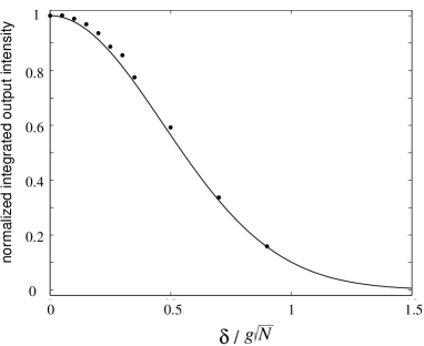
One recognizes that the two-photon linewidth of the “light storage” process $\delta_{\rm 2ph}$ is proportional to the collective Rabi-frequency. Thus in an optically thick medium rather large two-photon detunings can be tolerated. This is illustrated in Fig.3, where we have plotted the normalized integrated intensity of the polariton after storage and release, obtained from a numerical solution of the SVEA Maxwell-Bloch equations (2-9) and (11), as function of $\epsilon_{2}=\delta/g\sqrt{N}$.

FIG. 3.: Integrated output intensity of the polariton as function of $\delta/(g\sqrt{N})$ normalized to its value at $\delta=0$ obtained from a numerical solution of the Maxwell-Bloch equations (large dots) for the Gaussian input pulse and $\theta(t)$ of Fig.2 and for $\gamma/(g\sqrt{N})=1$. The full line shows the analytic approximation (31).

IV summary

We have derived an analytic expression for the two-photon linewidth of storage and retrieval of light pulses by stimulated Raman adiabatic passage which is in excellent agreement with exact numerical simulations. We have shown that the transfer process tolerates a rather large two-photon detuning if the medium is optically thick. This allows the application of the light-storage technique to systems with a non-vanishing inhomogeneously broadened two-photon transition.

REFERENCES

- [1] D.P. DiVincenzo, Fortschr. Physik, 48, 771 (2000).
- [2] M. D. Lukin, S. F. Yelin, and M. Fleischhauer, Phys. Rev. Lett. 84, 4232 (2000).
- [3] M. Fleischhauer and M. D. Lukin, Phys. Rev. Lett. 84, 5094 (2000);
- [4] M. Fleischhauer and M. D. Lukin, Phys. Rev. A. 65, 022314 (2002);
- [5] S. E. Harris, Physics Today 50, 36 (1997).
- [6] K. Bergmann, H. Theuer, and B. W. Shore, Rev. Mod. Phys. 70, 1003 (1998); N. V. Vitanov, M. Fleischhauer, B. W. Shore, and K. Bergmann, Adv. Atom. Mol. Opt. Physics 46, 55 (2001).
- [7] C. Liu, Z. Dutton, C.H. Behroozi, and L.V. Hau, Nature 409, 490 (2001).
- [8] D. F. Phillips, A. Fleischhauer, A. Mair, R. L. Walsworth, and M. D. Lukin, Phys. Rev. Lett. 86, 783 (2001).
- [9] G. Juzeliunas and H. J. Carmichael, Phys. Rev. A 65, 021601(R) (2002)
- [10] A. S. Zibrov, A. B. Matsko, O. Kocharovskaya, Y. V. Rostovtsev, G. R. Welch, and M. O. Scully, Phys. Rev. Lett. 88, 103601 (2002).
- [11] A. V. Turukhin, V. S. Sudarshanam, and M. S. Shahriar, J. A. Musser, B. S. Ham, and P. R. Hemmer, Phys. Rev. Lett. 88, 023602 (2002).