Time scale of forerunners in quantum tunneling

Abstract

The forerunners preceding the main tunneling signal of the wave created by a source with a sharp onset or by a quantum shutter, have been generally associated with over-the-barrier (non-tunneling) components. We demonstrate that, while this association is true for distances which are larger than the penetration lenght, for smaller distances the forerunner is dominated by under-the-barrier components. We find that its characteristic arrival time is inversely proportional to the difference between the barrier energy and the incidence energy, a tunneling time scale different from both the phase time and the Büttiker-Landauer (BL) time.

I INTRODUCTION

Tunneling is one of the paradigms of quantum theory. Textbooks only discuss its stationary aspects, emphasizing the non-vanishing transmission probability for monochromatic wavefunctions with energies below the barrier maximum. In recent times, since the seminal work of Büttiker and Landauer BL82 , its time dependent aspects have been also investigated to find characteristic time scales that summarize, together with the transmittance, the system behavior. Much of this work has been controversial, as several authors have proposed and defended different “tunneling times”. In fact each has its own virtues, weaknesses, and range of applicability. For a recent and rather extensive multi-author review see MSE02 ; for previous reviews see HS89 ; LA90 ; LM94 ; Ghose99 . An analysis of the involved non-commuting observables (the projectors that determine the final transmission and the probability to find the particle in the barrier region) shows that, from a fundamental perspective, there is no unique tunneling time, because several quantizations are possible due to different operator orderings and defining criteria BSM94 .

This does not mean though that the timing question should be abandoned. Rather, it is necessary to specify more precisely how to time the quantum particle in the tunneling regime. Different specifications lead to different relevant time scales; in other words, the importance of the differently defined times rests on the context where they become physically significant quantities. For example, the traversal time of Büttiker and Landauer (BL time)BL82 , $\tau=L/v_{sc}$, given by the barrier length $L$ divided by the “semiclassical” velocity $v_{sc}=[2(V-E)/m]^{1/2}$, marks the transition from sudden to adiabatic regimes for an oscillating barrier BL82 , and determines the rotation of the spin in a weak magnetic field in opaque conditions Buttiker83 ; whereas the average over wavepacket components of the (monochromatic) “phase times” provides the mean arrival time of the transmitted wave packet BSM94 ; ML00 . These two time scales may be very different. The Büttiker-Landauer time increases with decreasing energies up to a finite value, whereas $\tau^{Ph}(0,L)$ (the so called extrapolated phase time) diverges as $E\to 0$, and tends for increasing $L$ to a constant value, $2\hbar/[v_{sc}(2mE)^{1/2}]$. This later property implies that the arrival of the transmitted wave becomes independent of $L$ (Hartman effect Hartman62 ), although the independence only holds until a certain critical length $L_{c}$ BSM94 where above-the-barrier components start to dominate. For $L>L_{c}$ the mean arrival time depends on $L$ linearly. While $\tau$ and $\tau^{Ph}$ are surely the most frequently invoked tunneling times, they do not exhaust all timing questions.

In particular, in Ref. MB00 , the time $t_{tr}=t_{tr}(x)$ that characterizes the transition from the transient to the stationary regime for a wave formed by a point source with a sharp onset, was identified and the time of arrival, $t_{p}=t_{p}(x)$, of the peak of the forerunner at a point $x$ in opaque conditions was also identified. Here “opaque” means $x\kappa_{0}\gg 1$, where $\kappa_{0}=[2m(V-E_{0})]^{1/2}/\hbar$, and $E_{0}=\hbar\omega_{0}$. This particular time scale turned out to be (surprisingly) proportional to the BL time $\tau$ i.e.,

$$t_{p}=\tau/3^{1/2},$$ (1)

even though the time-frequency analysis of the forerunner showed that it was composed by frequencies above threshold. In other words, it corresponded to non-tunneling. In spite of its frequency content, the forerunner’s peak “travels” with a velocity proportional to $v_{sc}$, $v_{p}=3^{1/2}v_{sc}$, which increases with decreasing energies, and its intensity diminishes exponentially as it progresses along the coordinate $x$. Other works had already pointed out the dominance of non-tunneling components in the forerunner RMFP90 ; RMA91 ; TKF87 ; APJ89 ; BM96 but had not characterized its time dependence. Their main objective was to show that a previous prediction by Stevens Stevens (who believed that a tunneling monochromatic $\omega_{0}$-front, associated with a pole at $\omega_{0}$ in the complex frequency plane would arrive at $\tau$) did not hold because of the effect of the saddle point or other critical points, such as resonances in a square barrier model BM96 . (For the source-with-a-sharp-onset model the frequency of the saddle is given by $\omega_{s}=E_{s}/\hbar$, where the saddle energy, $E_{s}=V+x^{2}m/2t^{2}$, coincides with the energy of a classical particle traveling from the source to $x$ in a time $t$.) Büttiker and Thomas BT proposed to enhance the importance of the monochromatic front associated with $\omega_{0}$ compared to the forerunners by limiting the frequency band of the source or of the detector; it was shown later in MB00 that the monochromatic front could not be seen in opaque conditions even with the frequency band limitation. However, a clear separation of the amplitude into two terms, one associated with saddle and forerunner and the other with the pole and the “monochromatic front”, is only possible for opaque conditions. Non semiclassical conditions have been much less investigated Nimtz , even though these are actually easier to observe because of the stronger signal. In this paper we shall be mainly concerned with them.

The motivation of the present paper is a recent publication of two of us where the time evolution of an initial cutoff wave truncated at the left edge of a square barrier (shutter problem) gcv01 was examined. There it was found that the probability density at the barrier edge $x=L$, exhibits at short times a transient structure named time domain resonance. The maximum, $t_{p}$, of the time domain resonance showed a plateau region for small $L$, or more accurately a shallow basin, followed by a linear dependence for larger $L$; this behavior is reminiscent of the Hartman effect, but the time of the plateau did not coincide with the phase-time estimate. It was found that for a broad range of parameters, $t_{p}$ in the basin may be written approximately as,

$$t_{p}^{B}=\frac{\hbar\pi}{\epsilon_{1}-E_{0}},$$ (2)

where $\epsilon_{1}$ and $E_{0}$, correspond to the energy of the first top-barrier resonance and the incidence energy, respectively. Such a dependence had not been described before. On the other hand, along the linear regime, at larger values of $L$, $t_{p}$ is described by,

$$t_{p}^{L}=\frac{L}{v_{1}},$$ (3)

where $v_{1}=\hbar a_{1}/m$, with $a_{1}$ the real part of the first top-barrier pole $k_{1}=a_{1}-ib_{1}$. The above time scales are also different from the BL-time, even though they may coincide with $t_{p}^{L}$ for a particular value of $L$.

We shall show in this paper that this basin dependence, and the corresponding time scale, is not only present at the transmission edge of the square barrier studied in gcv01 . It may also be found, mutatis mutandis, in the sharp onset source model examined in MB00 for small $x\kappa_{0}$. We also find the basin for the time of the forerunner versus position in the internal region of the square barrier, and for a step potential barrier. There are not resonances in the sharp onset source model, or for the step potential, so the time scale of the basin minimum is in these cases inversely proportional to $\kappa_{0}^{2}$, namely to the difference between the “potential level” $V$ and the source main energy $E_{0}$. This is to be contrasted with the dependence on $\kappa_{0}^{-1}$ of the traversal time $\tau$.

An important open question was to determine if the forerunner at small lengths in the evanescent region corresponds or not to tunneling frequencies. We shall show by a simple time-frequency analysis that the peak of the forerunner in this regime is composed predominantly by under-the-barrier components, so that indeed a genuine tunneling time scale different from phase or BL times has been found.

In section II the source with a sharp onset is discussed, and in section III we shall examine the internal region of the square barrier, as well as the step barrier case. As the reader will soon discover, apart from certain peculiarities, all models show a small length region of the order of the penetration length $\kappa_{0}^{-1}$ where the forerunner is dominated by tunneling components and arrives at a time proportional to $\kappa_{0}^{-2}$.

II SOURCE WITH A SHARP ONSET

II.1 Formalism

The time dependent solution of the Schrödinger equation for a potential $V(x)=V$ that occupies the entire space, subject to a source boundary condition,

$$\psi(0,t)=e^{-i\omega_{0}t/\hbar}\Theta(t),$$ (4)

has the form, MB00

$$\Psi(x,t)=\frac{1}{2}e^{-itV/\hbar+ix^{2}/(4C^{2}t)}\left[w(-u_{0}^{\prime})+w(-u_{0}^{\prime\prime})\right],$$ (5)

where $w(z)=e^{-z^{2}}{\rm erfc}(-iz)$ and

$$u_{0}^{\prime} = \frac{1+i}{2^{1/2}}t^{1/2}C\kappa_{0}\left(-i-\frac{\tau}{t}\right),$$ (6)

$$u_{0}^{\prime\prime} = \frac{1+i}{2^{1/2}}t^{1/2}C\kappa_{0}\left(i-\frac{\tau}{t}\right),$$

$$\tau = x/v_{sc}=xm/\kappa_{0}\hbar,$$ (7)

$$C = (\hbar/2m)^{1/2}.$$ (8)

In the opaque limit ($x\kappa_{0}\gg 1$), an excellent approximation is given by adding up the pole and saddle terms,

$$\Psi(x,t) \approx \Psi_{0}+\Psi_{s},$$ (9)

$$\Psi_{0} = e^{-i\omega_{0}t}e^{-\kappa_{0}x}\Theta(t-\tau),$$ (10)

$$\Psi_{s} = \frac{1}{2i\pi^{1/2}}e^{-\frac{itV}{\hbar}+\frac{ix^{2}}{4C^{2}t}}\left(\frac{1}{u_{0}^{\prime}}+\frac{1}{u_{0}^{\prime\prime}}\right).$$ (11)

For opaque conditions at fixed $x$ the saddle term is totally dominant in the forerunner peak; at later times it fades away and the pole (tunneling) term becomes dominant. This allowed to identify $t_{p}$ from the peak of $|\Psi_{s}|^{2}$, and $t_{tr}$ as the time where the two contributions were of equal importance. The small $x\kappa_{0}$ regime did not permit the same approximation treatment, so that $t_{p}$ could not be characterized by the formula found for the opaque case, Eq. (1). It may be argued however, that the small $x\kappa_{0}$ case is in fact more interesting since it allows non-negligible signals (densities), whereas for large opacity the signal becomes exponentially small and very hard to detect.

II.2 Examples

In Fig. 1 we have depicted the density versus $t$ for a fixed $x$ smaller than the penetration length $1/\kappa_{0}$ for the source-with-a-sharp-onset model. In all calculations the effective mass of the electron is taken as $m=0.067m_{e}$. The forerunner is identified as a smooth broad bump with its peak at $t_{p}$. The contributions of the saddle and pole terms are also drawn, as well as the contribution of their sum. The saddle term reproduces the density only for very short times while the pole gives the large time behavior.

Figure 1: $|\Psi|^{2}$ (solid line), $|\Psi_{s}|^{2}$ (circles), $|\Psi_{0}|^{2}$ (dashed line), and $|\Psi_{0}+\Psi_{s}|^{2}$ (dotted-dashed line) versus $t$ for $E_{0}=0.907V$, and $x=2.75$ nm. Here and in Figs. 2-6, $V=0.3$ eV. In all figures $m=0.067m_{e}$, where $m_{e}$ is the electron’s mass.

Figure 2: $\omega_{av}/\omega_{V}$ (solid line), $\omega_{0}/\omega_{V}$ (dashed line), and $\omega_{s}/\omega_{V}$ (circles) versus $t$ for the same parameters of Fig. 1. The square marks the value of $t_{p}$.

In Fig. 2 the average local frequency Cohen95 ; MB00 , $\omega_{av}=-\textrm{Im}\left[(d\Psi/dt)/\Psi\right]$, the frequency of the saddle $\omega_{s}$, and $\omega_{0}$ are shown, relative to $\omega_{V}$, versus $t$ for the same value of $x$. Note that $\omega_{av}$ tends to $\omega_{0}$ for large $t$, and to $\omega_{s}$ for very short times, going from $\omega_{s}$ to $\omega_{0}$ during the time span of the forerunner bump (compare with the density in Fig. 1); in particular $\omega_{av}/\omega_{V}<1$ at the peak $t_{p}$.

Figure 3: time of arrival of the forerunner’s peak versus $x$ for $\omega_{0}/=0.907\omega_{V}$ (upper solid line), and $\omega_{0}=0.544\omega_{V}$ (lower solid line). The upper and lower dashed lines are the corresponding BL-times. The values of $1/\kappa_{0}$ are also shown with a square ($\omega_{0}=0.544\omega_{V}$) and a circle ($\omega_{0}=0.907\omega_{V}$)

Fig. 3 shows the dependence with $x$ of the time of arrival of the peak of the forerunner, $t_{p}$, for two different values of $\omega_{0}$. The (unsharp) transition between the quasi-plateau region at lower $x$ and the linear regime for larger $x$ occurs around a few penetration lengths $1/\kappa_{0}$. Thus, a smaller $\omega_{0}$ implies a more reduced plateau. Also shown are the corresponding Büttiker-Landauer times for comparison. In the plateau region the forerunner’s peak does not travel but arrives roughly simultaneously at all $x$ (in fact up to the basin minimum the forerunner arrives earlier at larger $x$!); beyond the plateau region the forerunner, whose peak is characterized in that case by Eq. (1), arrives later at larger $x$, and becomes dominated by frequencies “above the barrier”.

Fig. 4 shows the average frequency $\omega_{av}$ calculated right at the forerunner’s peak at the time $t_{p}(x)$ for each value of $x$, as well as $\omega_{s}$, and $\omega_{0}$, all relative to $\omega_{V}$, for the same two values of $\omega_{0}$ of the previous figure. The forerunner’s peak frequency begins at $\omega_{0}$ at $x\to 0$, then it grows smoothly and becomes non-tunneling ($\omega_{av}/\omega_{V}$ crosses $1$) around $1/\kappa_{0}$. For larger $x$, $\omega_{av}$ tends to the saddle frequency $\omega_{s}$.

Figure 4: $\omega_{av}/\omega_{V}$ (solid line), $\omega_{0}/\omega_{V}$ (short dashed line), and $\omega_{s}/\omega_{V}$ (circles) for the same cases of Fig. 3. Upper curves: $\omega_{0}=0.907\omega_{V}$; lower curves: $\omega_{0}=0.544\omega_{V}$. The values of $\kappa_{0}^{-1}$ are indicated as in Fig. 3

Further insight into the nature of the tunneling forerunner is obtained by looking at a series of snapshots of the wave density versus $x$ (instead of looking at density versus time for a fixed location). The plateau, or rather shallow basin, must be, according to Fig. (3), the result of a “breathing” transient mode of the evanescent wave, which implies an essentially simultaneous growth of the wave for all $x$ up to a few penetration lengths, and until the maximum is achieved at $t_{p}$. This is indeed confirmed in Fig 5, where several snapshots of the density are taken at five different times. In the final one the wave is already close to its asymptotic (large time) form.

Figure 5: Density $|\Psi|^{2}$ versus $x$ for $\omega_{0}/\omega_{V}=0.907$ and $t=0.05,\,24,\,48,\,72$ and $97$ ns (solid, short-dashed, long-dashed, dot-dashed, and circles respectively).

The linear dependence of the time of arrival of the peak with $\kappa_{0}^{-2}$ is shown in Fig. 6, which is drawn by choosing the values of $V-E_{0}$ and $t_{p}$ corresponding to the minima of the shallow basins obtained for different values of $E_{0}$ (see Fig. 3).

Figure 6: Time of arrival of the forerunner’s peak $t_{p}$ versus $1/(V-E_{0})$ at the position that minimizes $t_{p}$ for a given $E_{0}$, see Fig. 3. As in all the figures of this section, $V=0.3$ eV.

III QUANTUM SHUTTER

III.1 Formalism

Assume now an arbitrary potential $V(x)$ ($0\leq x\leq L$) that vanishes outside the internal region, and the initial condition,

$$\Psi\left(x,k;t=0\right)=\left\{\begin{array}[]{cc}e^{ikx}-e^{-ikx},&\quad-\infty<x\leq 0,\\ 0,&\quad x>0,\end{array}\right.$$ (12)

which corresponds to a plane wave impinging on a perfectly reflecting shutter placed at $x=0$, just at the left edge of the structure. The time dependent process begins with the instantaneous opening of the shutter at $t=0$, enabling the incoming wave to interact with the potential at $t>0$. The exact solution along the internal region ($0\leq x\leq L$) is given by gcr97 ,

$$\Psi^{i}=\phi_{k}M(y_{k})-\phi_{-k}M(y_{-k})-\sum\limits_{n=-\infty}^{\infty}\rho_{n}M(y_{k_{n}}).$$ (13)

In the above expressions, the quantities $\phi_{\pm k}$ refer to the stationary solution, and the factor $\rho_{n}=2iku_{n}(0)u_{n}(x)/(k^{2}-k_{n}^{2})$ is given in terms of the resonant eigenfunctions, $\{u_{n}(x)\}$, with complex eigenvalues gcr97 $k_{n}=a_{n}-ib_{n}$ ($a_{n},b_{n}>0$).

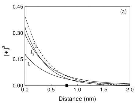
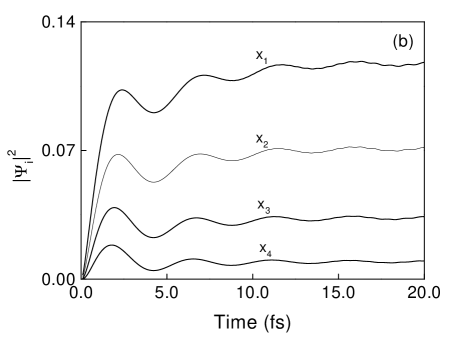
Figure 7: (a) Snapshots of $|\Psi^{i}|^{2}$ (solid line) taken at different values of time: $t_{1}=1.0$ fs, $t_{2}=2.0$, and $t_{3}=4.0$ fs. The stationary solution $|\phi_{k}|^{2}$ is included for comparison, and a full square indicates the value of $\kappa_{0}^{-1}$, which is the penetration length of the stationary solution. (b) Time evolution of $|\Psi^{i}|^{2}$ at different fixed values of the position $x$: $x_{1}=0.5$ nm, $x_{2}=0.7$ nm, $x_{3}=1.0$ nm, and $x_{4}=2.0$ nm. The solution exhibits a behavior similar to diffraction in time pattern.

The index $n$ runs over the complex poles $k_{n}$, distributed in the third and fourth quadrants in the complex $k$-plane. Both the complex poles $\{k_{n}\}$ and the corresponding resonant eigenfunctions $\{u_{n}(x)\}$, can be calculated using a well established method, as discussed elsewhere gcr97 ; gcv01 . In the above equation the $M$ functions are defined as,

$$M(y_{q})=\frac{1}{2}w(iy_{q}),$$ (14)

where $y_{q}=-e^{-i\pi/4}[(\hbar/2m)t]^{1/2}q$, $q=\pm k$, and $k_{\pm n}$.

III.2 Examples

In what follows we shall explore the features of the probability density along the internal region of one-dimensional rectangular potential barriers of height $V$ and thickness $L$, defined along the interval $0\leq x\leq L$. We choose the following parameters: $V=1.0$ eV, $L=40.0$ nm, and incidence energy $E_{0}=\hbar^{2}k^{2}/2m=0.1$ eV. For this particular case the full barrier is opaque, $\alpha\equiv L[2mV]^{1/2}/\hbar=53.0$, but we are interested in distances of the order of, or smaller than, the penetration length $\kappa_{0}^{-1}<<L$.

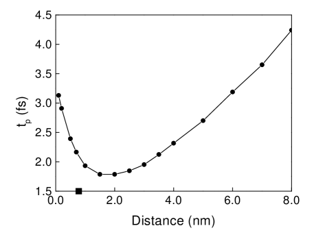
Figure 8: Exact calculation of $t_{p}$ (solid dots) as a function of the position $x$. The parameters are the same as in Fig. 7. A full square indicates the value of $\kappa_{0}^{-1}$.

In Fig. 7 (a) we use Eq. (13) to explore the birth of the probability density along the internal region of the potential. Here we plot $|\Psi^{i}|^{2}$ (solid line) as a function of small values of the position $x$, for increasing values of time. Notice that as time increases, the probability density evanesces along the internal region swinging around the stationary solution (dashed line).

In Fig. 7 (b) we illustrate the time dependence of the transient “swinging mode” exhibited in Fig. 7 (a). We exhibit the behavior of $|\Psi^{i}|^{2}$ (solid line) as a function of time for several values of the position $x_{i}$ ($i=1,2,3,4$). The probability density grows monotonically until it reaches its first maximum value, and oscillates thereafter as it tends to the stationary situation given by $|\phi_{k}|^{2}$gcr97 . Here we observe again a peculiar behavior in the time evolution of $|\Psi^{i}|^{2}$, presented in plot (b) of Fig. 7: the first maximum of the probability density appears earlier at larger values of $x$. In Fig. 8 we plot the exact calculation of $t_{p}$ (solids dots), which corresponds to the peak value of the first maximum of $|\Psi^{i}|^{2}$, measured at different values of the position, $x$.

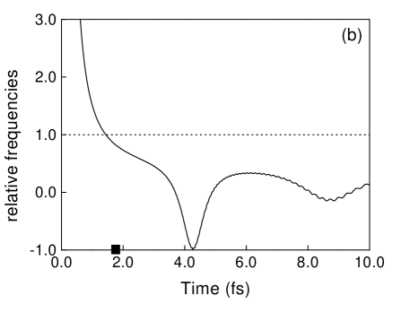
Figure 9: Plot of the relative local frequency $\omega_{av}/\omega_{V}$ (solid line) for the positions (a) $x_{1}=0.5$ nm, , and (b) $x_{4}=2.0$ nm, corresponding to the cases depicted in Fig. 7 (b). The cutoff-frequency $\omega_{V}/\omega_{V}=1$ (dotted line) is included for comparison, and a full square indicates the position of $t_{p}$.

In Fig. 8 we can clearly identify two regimes, as in the case of Fig. 3. The first of them corresponds to a basin, where for small values of the position, $t_{p}$ decreases reaching a minimum value as $x$ increases. This is in accordance with the observed behavior of the maximum in Fig. 7 (b). However, if $x$ is further increased, $t_{p}$ begins to grow as a function of the position. Apparently this second regime corresponds to a situation where $t_{p}$ increases linearly with $x$. The result depicted in Fig. 8 appears to be a replica of a similar behavior of the probability density at the barrier edge $x=L$, recently reported in Ref. gcv01 .

We have also analyzed the frequency content of $|\Psi^{i}|^{2}$ along the internal region. In Fig. 9 (b) we plot $\omega_{av}/\omega_{V}$ along the relevant time interval for some of the values of the position, depicted in Fig. 7 (b). We can appreciate that the probability density at this small values of the position $x$, is composed entirely by under-the-barrier frequency components i.e $\omega_{av}/\omega_{V}<1$ in the vicinity of the maximum $t_{p}$. Notice that this result is similar to the one obtained in Fig. 2.

Finally, Fig. 10 shows the linear dependence of the time corresponding to the basin minimum with respect to $1/(V-E_{0})$ in analogy to the analysis of the point source problem. Note, however, that in our case we could also have considered a plot with respect to $1/(\varepsilon_{1}-E_{0})$ with a similar result since it turns out that for opaque barriers $\varepsilon_{1}\approx V$.

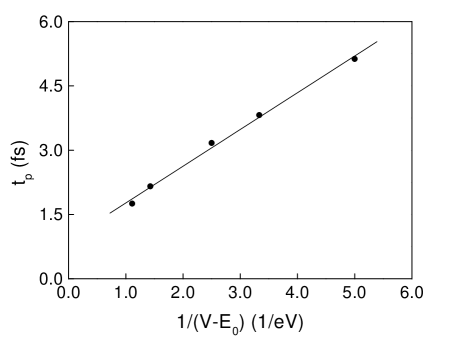
Figure 10: Maximum of the time domain resonace, $t_{p}$, as a function of $1/(V-E_{0})$. The parameters are the $V=1.0$ eV, and $L=40.0$ nm.

III.3 Potential step

Figure 11: $\omega_{av}/\omega_{V}$ (solid line), $\omega_{0}/\omega_{V}$ (dotted line), and $\omega_{s}/\omega_{V}$ (dashed line) for $V=1$ eV and $E_{0}=0.5$ eV. The value of $\kappa_{0}^{-1}$ is indicated with a square.

The potential step $V\Theta(x)$ requires a different formal treatment muga02 but very similar results are found. We have evaluated $\langle x|\Psi(t)\rangle$ by means of an integral over the energy eigenfunctions for the the initial state,

$$\Psi\left(x,k;t=0\right)=\left\{\begin{array}[]{cc}e^{ikx},&\quad-\infty<x\leq 0,\\ 0,&\quad x>0.\end{array}\right.$$ (15)

In Fig. 11 the average frequency peak of the forerunner is shown versus $x$ for this system. As in the source with a sharp onset case, it goes from $\omega_{0}$ to $\omega_{s}$, crossing the threshold frequency at approximately $2/\kappa_{0}$. Fig. 12 shows also the linear dependence of the time of the forerunner (calculated at its minimum value for a given energy, i.e., at the basin minimum) versus $1/(V-E_{0})$.

Figure 12: Time of arrival of the forerunner’s peak $t_{p}$ versus $1/(V-E_{0})$ at the position that minimizes $t_{p}$ for a given $E_{0}$. $V=1$ eV.

IV Final comments

By using different time-dependent models of quantum waves impinging on a potential barrier, we have shown the existence of forerunners dominated by under-the-barrier components. This transient structures are indeed associated with a true tunneling process, occurring at distances smaller than the penetration length, $\kappa_{0}^{-1}$. We find that the time of arrival is proportional to $1/(V-E_{0})$, where $E_{0}$ stands for the incidence energy, chosen below the barrier height, $V$. This is in contrast to the dominance of above the barrier frequencies for larger distances, and to other well known tunneling time scales such as the Büttiker-Landauer or “phase” times.

These results suggest a number of questions that need further investigation. For example, the proportionality constant observed in the arrival times of the forerunner’s peak, depends on the peculiarities of each model, and a general theory for its specific value should be found. Also, the Larmor time for spin rotation defined by Büttiker is given for very thin barriers by $\hbar/V$ in the limit $k=0$ Buttiker83 . In spite of the very different ways in which the Larmor time and the forerunner’s peak time are obtained, these two quantities might be related. Finally, we hope that the results presented may motivate an experimental search of tunneling forerunners and their corresponding time scale.

- (1) M. Büttiker and R. Landauer, Phys. Rev. Lett. 49, 1739 (1982).
- (2) Time in Quantum mechanics, J. G. Muga, R. Sala, I. L. Egusquiza (eds.) (Springer-Verlag, Berlin, 2002).
- (3) E.H. Hauge, J.A. Stovneng, Rev. Mod. Phys. 61, 917 (1989).
- (4) C.R. Leavens, G.C. Aers: in Scanning Tunneling Microscopy and Related Techniques, ed. by R. J. Behm, N. García, H. Rohrer (Kluwer, Dordrecht, 1990)
- (5) R. Landauer and Th. Martin, Rev. Mod. Phys. 66, 217 (1994)
- (6) P. Ghose, Testing Quantum Mechanics on New Ground (Cambridge University Press, Cambridge, 1999), Chapter 10.
- (7) S. Brouard, R. Sala and J. G. Muga, Phys. Rev. A 49, 4312 (1994).
- (8) M. Büttiker, Phys. Rev. B. 27, 6178 (1983).
- (9) J. G. Muga and C. R. Leavens, Phys. Rep. 338, 353 (2000).
- (10) T. E. Hartman, J. Appl. Phys. 33, 3427 (1962).
- (11) J. G. Muga and M. Büttiker, Phys. Rev. A 62, 023808 (2000).
- (12) A. Ranfagni, D. Mugnai, P. Fabeni and P. Pazzi, Physica Scripta 42, 508 (1990).
- (13) A. Ranfagni, D. Mugnai and A. Agresti, Phys. Lett. A 158, 161 (1991).
- (14) N. Teranishi, A. M. Kriman and D. K. Ferry, Superlattices and Microstructures, 3, 509 (1987).
- (15) A. P. Jauho and M. Jonson, Superlattices and Microstructures 6, 303 (1989).
- (16) S. Brouard and J. G. Muga, Phys. Rev. A 54, 3055 (1996).
- (17) K. W. H. Stevens, Eur. J. Phys. 1, 98 (1980); J. Phys. C: Solid State Phys. 16, 3649 (1983).
- (18) M. Büttiker and H. Thomas, Ann. Phys. (Leipzig) 7, 602 (1998); Superlattices Microstruct. 23, 781 (1998).
- (19) G. Nimtz, A. Haibel, and R. M. Vetter, in Time’s arrows, quantum measurement and superluminal behaviour, (C.N.R., Roma, 2001) p. 125.
- (20) G. García-Calderón and J. Villavicencio, Phys. Rev. A 64 012107 (2001).
- (21) L. Cohen, Time-Frequency analysis (Prentice Hall, New Jersey, 1995).
- (22) G. García-Calderón and A. Rubio, Phys. Rev. A 55, 3361 (1997).
- (23) F. Delgado and J. G. Muga, unpublished results.