The Dirac Equation in Classical Statistical Mechanics

Abstract

The Dirac equation, usually obtained by ‘quantizing’ a classical stochastic model is here obtained directly within classical statistical mechanics. The special underlying space-time geometry of the random walk replaces the missing analytic continuation, making the model ‘self-quantizing’. This provides a new context for the Dirac equation, distinct from its usual context in relativistic quantum mechanics.

1 Introduction

The title of this talk requires some explanation. Statistical mechanics is in some respects the simplest branch of physics; all you ever have to do is count. The trick is of course to find the right class of objects to count.

The implication of the title is that the Dirac equation is simply related to the operation of counting objects. If we were talking about the diffusion or heat equation then there would be no mystery. It is well known that the diffusion equation may be obtained by counting random walks in an appropriate limit.

However, the likelihood of being able to make a similar claim for the Dirac equation seems small. We all know that the Dirac equation has elements of quantum mechanics, special relativity and half-integral spin. None-the-less the claim in the title is true for the Dirac equation in one dimension [1], and may well be true in three dimensions for a free particle. Among other things, this means that the Dirac equation has a context as a phenomenology which may be distinct from its role as a fundamental equation of quantum mechanics. Although this may be surprising from the perspective of quantum mechanics, it is not so extraordinary in the context of general partial differential equations. For example we are used to calling the same PDE either the Diffusion equation or the heat equation, depending on context. In the case of Dirac, we have only one name for the equation, but there are still multiple contexts.

Today I am going to talk about the Dirac equation as a classical phenomenology. However since we all think ‘quantum mechanics’ at the mention of Dirac’s name, let’s recall where Quantum mechanics begins and where it ends. Typically we pass from classical physics to quantum mechanics through a formal analytic continuation (FAC). The canonical FAC is to replace the momentum by the operator $-i\hbar\nabla$ and the energy by $i\hbar\frac{\partial}{\partial t}$. In a sense this is where quantum mechanics begins and classical physics ends.

The quantum equations describe the evolution of the initial conditions in time, and we relate the results of this evolution to our macroscopic world by the measurement postulates. These postulates are the weakest link in the theory, and it is here that the (many) interpretations of quantum mechanics vie for supremacy. At this point we do not really know where quantum mechanics ends and classical physics begins. So let us return to the point where it begins, at the FAC.

The the canonical FAC just mentioned specifically relates the Schrödinger equation to Hamiltonian mechanics. We will not be so specific. Table(1) compares classical PDE’s with their corresponding ‘quantum’ counterparts. In the left ‘Classical’ column we start out with a two component form of the Telegraph equations due to Marc Kac. Here U is related to a two component probability density, $c$ is a mean free speed and $a$ is an inverse mean free path. Note that if we replace the real positive constant $a$ by $im$ we get a form of the Dirac equation.

	Classical	Quantum
Microscopic basis	Kac (Poisson)	Chessboard
First Order	$\frac{\partial{\bf U}}{\partial t}=c\mbox{\boldmath$\sigma$}_{z}\frac{\partial\mathbf{U}}{\partial z}+a\mbox{\boldmath$\sigma$}_{x}\mathbf{U}$	$\frac{\partial\mathbf{\Psi}}{\partial t}=c\,\mbox{\boldmath$\sigma$}_{z}\frac{\partial}{\partial z}\mathbf{\Psi}+i\,m\mbox{\boldmath$\sigma$}_{x}\mathbf{\Psi}$
Second Order	$\frac{\partial^{2}U}{\partial t^{2}}=c^{2}\frac{\partial^{2}U}{\partial z^{2}}+a^{2}U$	$\frac{\partial^{2}\psi}{\partial t^{2}}=c^{2}\frac{\partial^{2}\psi}{\partial z^{2}}-m^{2}\psi$
‘Non-relativistic’	$\frac{\partial U}{\partial t}=D\,\frac{\partial^{2}U}{\partial x^{2}}$	$\frac{\partial\psi}{\partial t}=i\,D\,\frac{\partial^{2}\psi}{\partial x^{2}}$

Table 1: The relation between Classical PDE’s based on stochastic models, and their ‘Quantum’ cousins. FAC accomplishes the trick, but then the stochastic basis for the equations becomes formal.

Similarly the second order form of the Telegraph equations continues to the Klein-Gordon or Relativistic-Schrödinger equation using the same FAC. The ‘non-relativistic limit’ of the Telegraph equation gives the Diffusion equation, with the usual FAC to the Schrödinger equation. The equations on the left are phenomenologies which are interpreted through the underlying statistical mechanical models (Poisson or Brownian motion). The equations on the right are regarded as fundamental equations which have no realistic microscopic basis, and are interpreted through postulates. The analog of Poisson paths for the Telegraph equations are the Chessboard paths of Feynman.

What we will do today is to show that the Dirac equation in 1-dimension is also a phenomenological equation with a microscopic basis, and is accessible directly through classical statistical mechanics …all we have to do is to find the right objects to count. But first let us see how Kac[2] obtained the Telegraph equations from a microscopic model.

2 The Kac Model

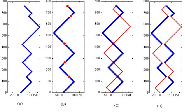
Imagine a particle on a discrete space-time lattice with spacings $\Delta z$ and $\Delta t$. The speed of particles are fixed at $c$ and occasionally they scatter backwards with probability $\alpha\Delta t$. Fig. (1.A) shows a typical Kac path. Considering the density of particles moving in the plus and minus directions we can write difference equations for their conservation.

$$F_{n}^{+}(z)=(1-a\Delta t)F_{n-1}^{+}(z-c\Delta t)+a\Delta tF_{n-1}^{-}(z)$$ (1)

Similarly,

$$F_{n}^{-}(z)=(1-a\Delta t)F_{n-1}^{-}(z+c\Delta t)+a\Delta tF_{n-1}^{+}(z)$$ (2)

In the continuum limit these give the coupled PDE’s:

$$\frac{\partial F^{+}}{\partial t}=-c\frac{\partial F^{+}}{\partial z}-aF^{+}+aF^{-}$$ (3)

$$\frac{\partial F^{-}}{\partial t}=c\frac{\partial F^{-}}{\partial z}+aF^{+}-aF^{-}$$ (4)

It is easy to identify the streaming and scattering terms here, but if we remove the exponential decay, and write in 2-component form we get.

$$\frac{\partial\mathbf{U}}{\partial t}=c\mbox{\boldmath$\sigma$}_{z}\frac{\partial\mathbf{U}}{\partial z}+a\mbox{\boldmath$\sigma$}_{x}\mathbf{U}$$ (5)

where the $\sigma$  are the usual Pauli Matrices.

Note the suggestive form of the coupled equations. We are a FAC away from the Dirac equation. However the FAC destroys any coherent interpretation of our microscopic model, so we will strictly avoid it!

Figure 1: (A) Paths in the Kac process are broken-line segments with slope $\pm c$. The average distance between corners is $1/a$.(B) The Kac Stochastic process with a stutter. (C) With the return Path (indicated by the thinner line). (D) The outer envelopes of the Entwined paths.

3 The Entwined Pair Model

As mentioned above, counting Kac Paths gives the telegraph equations. So what do we count if we want to go directly to the Dirac equation? And how is $i$ going to appear if we are not allowed a FAC? To answer the second question first, we do not need $i$ to get the quantum equations, we only need the fact that $i^{2}$=-1. This may seem like a trivial point but it is extremely important. To illustrate it, think of the even and odd parts of $e^{t}$ …these are $\cosh(t)$ and $\sinh(t)$. Now analytically continue and think of the even and odd parts of $e^{it}$. These are $\cos(t)$ and $i\sin(t)$. It is true that here $i$ distinguishes the even and odd parts, but the important effect of the analytic continuation is to produce the alternating signs in the series expansion of the trigonometric functions. It is the same in the quantum equations. We do not actually need $i$, what we need is the alternating pattern of sign that gives oscillatory behaviour, and we have to get it from the geometry of particle trajectories, not from a FAC.

Consider the Entwined paths of Fig(1. B-D). We will generate these with the same process we used to generate the Kac paths of Fig.(1. A), except here we will employ a periodic ‘stutter’. That is, wherever we would change direction in a Kac path, we alternately change direction or leave a marker in the entwined path. At the first marker past some specified time $t_{R}$, we reverse our direction in $t$ and follow the markers back to the origin. In Fig(1. C), the return path has a thinner line-width to distinguish it from the forward path. Even in Classical physics, particles which move backwards in time behave like anti-particles to a forward moving observer, so if we record (+1) as a charge carried on forward portions of the trajectory, we shall associate a -1 with the return portions. The task will then be to calculate the expected average charge deposited by an ensemble of these paths. Note that each entwined pair can be regarded as two osculating envelopes with a periodic colouring(Fig.1. D). Each envelope is just a Kac path. Each has the same statistics and geometry as a Kac path, the only difference is the periodic colouring. We can then set up a difference equation as we did for the Telegraph equations. This time there are 4 states instead of Kac’s 2 states. Fig.(2. A) shows the four possible states of an entwined pair and Fig.(2. B) shows a path evolving through two loops.

Figure 2: The four possible states of Entwined Pairs and two cycles of an Entwined Pair. Note the alternating signs in the envelope.

$$\phi_{n}^{1}(z) = (1-a\Delta t)\phi_{n-1}^{1}(z-c\Delta t)-a\Delta t\phi_{n-1}^{2}(z-c\Delta t)$$

$$\phi_{n}^{2}(z) = (1-a\Delta t)\phi_{n-1}^{2}(z+c\Delta t)+a\Delta t\phi_{n-1}^{1}(z+c\Delta t)$$

$$\phi_{n}^{3}(z) = (1-a\Delta t)\phi_{n-1}^{3}(z-c\Delta t)-a\Delta t\phi_{n-1}^{4}(z-c\Delta t)$$ (6)

$$\phi_{n}^{4}(z) = (1-a\Delta t)\phi_{n-1}^{4}(z+c\Delta t)+a\Delta t\phi_{n-1}^{3}(z+c\Delta t)$$

Note the alternating minus sign from the crossover of paths (cf. Feynman Chessboard Model). Here the $\phi$ are real ensemble averages of a net ‘charge’ density. They are not quantum mechanical amplitudes.

Removing the exponential decay and writing $p_{z}=-i\frac{\partial}{\partial z}$, setting $c=1$ and $a=m$ with $\alpha_{z}=\left(\begin{array}[]{c c}-\sigma_{z}&0\\ 0&\sigma_{z}\end{array}\right)$ $\beta=\left(\begin{array}[]{c c}\sigma_{y}&0\\ 0&\sigma_{y}\end{array}\right)$ we get the Dirac equation

$$i\frac{\partial\psi}{\partial t}=(\alpha_{z}.p_{z}+\beta m)\psi$$ (7)

in the continuum limit. Notice there is no FAC here. The $i$ in Eqn.(7) was introduced simply to show a familiar form of the Dirac equation. The $\psi$ here are real, four component, and oscillatory in character. The oscillation is implemented through the presence of $\sigma_{q}=i\sigma_{y}$, which is a real, anti-hermitian matrix. $\sigma_{q}$ arises because of the periodic exchange of particle and antiparticle in entwined paths, and it has the important feature that $\sigma_{q}^{2}=-1$. We have not forced an analytic continuation on the system here. The space-time geometry itself has rendered the system ‘self-quantizing’!

4 Discussion

The above suggests that the Dirac equation appears as an ensemble average of a net charge over our entwined pairs. Since all pairs meet at the origin the entire ensemble can be regarded as being generated by a single particle traversing all entwined paths. However the above analysis only shows that the Dirac propagator will result if we cover the ensemble exactly. There have been other cases where the quantum equations have been recovered as projections without using a FAC [3, 4, 5, 6, 7, 8], however all of these have required a complete ensemble. What happens if we just watch the stochastic process with its inherent fluctuations? Will the process converge to the propagator or will the fluctuations swamp the signal? The answer appears to be that the signal survives stochastic fluctuations. The Dirac propagator is a stable feature of entwined paths! Figures (3) and (4) show the propagator drawn by a single path in comparison to the discrete Dirac propagator.[1]

Figure 3: Contour plot of the sum of the real and imaginary parts of the Dirac Propagator. Left, discrete Dirac, right, single path.

Figure 4: A time slice through the above figure at $t=15$. The curve is the Dirac propagator and the black dots are the single path.

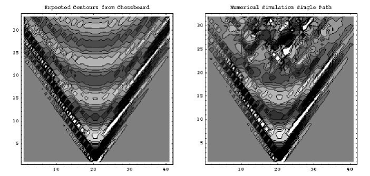
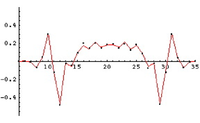
In Fig.(3) we see that the propagator formed by the entwined paths is quite accurate near the origin but gets less accurate the father out we go. This is to be expected since the configuration space grows exponentially as the number of time steps and the farther away we are from the origin, the poorer the ensemble coverage.

Considering the original context of the Dirac Equation, the above demonstration that the equation is easily obtained within classical statistical mechanics is surprising, to say the least. Clearly, the algebraic route followed by Dirac to obtain his equation was, and is, elegant, concise and algebraically compelling. However, for all its comparative inelegance, the heuristic approach via entwined paths strongly suggests that canonical quantization, Dirac’s starting point, might well benefit from a re-evaluation. The FAC represented by canonical quantization gives an algebraic connection to Hamiltonian mechanics without any suggestion as to what the connection actually means in terms of the propagation of a classical particle. By comparison, the entwined paths approach replaces a formal algebraic requirement by a physical constraint on space-time geometry. What we lose in elegance we may well regain in physical cogency. As Dirac suggested in the preface to his book[9]

“Mathematics is the tool specially suited for dealing with abstract concepts, …All the same, the mathematics is only a tool and one should learn to hold the physical ideas in one’s mind without reference to the mathematical form.”

References

- [1] G. N. Ord and J. A. Gualtieri. The feynman propagator from a single path. quant-ph 0109092, 2001.
- [2] M. Kac. A stochastic model related to the telegrapher’s equation. Rocky Mountain Journal of Mathematics, page 4, 1974.
- [3] G. N. Ord. Classical analog of quantum phase. Int. J. Theor. Physics, 31(7):1177–1195, 1992.
- [4] G. N. Ord. Quantum interference from charge conservation. Phys. Lett.A, 173:343–346, 1993.
- [5] G. N. Ord. The schrödinger and diffusion propagators coexisting on a lattice. J.Phys. A: Math. Gen., 29:L123–L128, 1996.
- [6] D. G. C. McKeon and G. N. Ord. Time reversal in stochastic processes and the dirac equation. Phys. Rev. Lett., 69(1):3–4, 1992.
- [7] G. N. Ord and A.S.Deakin. Random walks and schrödinger’s equation in 2+1 dimension. J.Phys.A, 30:819–830, 1997.
- [8] G. N. Ord and A.S.Deakin. Random walks, contimuum limits and schrödinger’s equation. Phys. Rev. A., 54(5):3772–3778, 1996.
- [9] P.A.M. Dirac. The Principles of Quantum Mechanics. Oxford at Clarendon Press, 1958.