Zero-Range Potentials in Multi-Channel Diatomic Molecule Scattering

Abstract

The method of zero-range potentials is generalized to account for the molecular electron excitation process. It is made by a matrix formulation in which a state vector components are associated with a scattering channel. The multi-center target is considered and the model is applied to the example of $e+H_{2}$ low energy scattering. The results of evaluation of cross-sections are compared with ones of the MCF and SMC methods.

1 Introduction.

The ideas of zero range potential (ZRP) approach were recently developed to widen limits of the traditional treatment [1], the author accounts higher momentum partial amplitudes [2] for a multi-center problem. Historically, the ZRP notion was introduced, perhaps, in [3] to model a potential action sustaining some parameters values. The simplification of the theory is such that a problem of differential equation goes down to some algebraic one [4]. There is the book [1] and the review [10] in which the theory is comprehensively described.

The target of this paper relates to the other limitation of the theory connected with multi-channel character of real scattering phenomenon. Following the ideas of [6] we introduce a vector formulation of the scattering problem with the components that stands for different possibilities (channels) of the process to be described. The scattering amplitude hence is a matrix connecting asymptotic states. In the Sec. 1 the formalism is introduced for a multi-center problem.

As an important example we consider applications to a diatomic molecule. In the framework of the generalization to be introduced we revisit results of the papers [5], [7] starting from adiabatic nuclei problem (Sec.2). The rotations of a molecule are included similarly to the mentioned approach [7] but with some difference in the formalism. Oscillations are described by means of the Morse potential with eigen functions - vibrational harmonics that are proportional to Laguerre polynomials (Appendix). The results of differential and integral cross-sections evaluation are compared with the direct numerical solution by some standard molecular orbits model [17] (Sec.3).

2 The matrix zero-range potentials

As it is known, if we diminish the range and at the same time increase the depth of a pertinent spherically symmetrical potential then the only characteristic parameter of a potential may remain fixed (usually it’s a scattering length or a position of the bound-state energy level), others characteristic are lost. This procedure allow to replace the potential action by the boundary condition on the wave function $\psi({\bf r})$ at the potential center (see Ref. [1, 8])

$$\left[\frac{\partial}{\partial\rho_{j}}\,\ln(\rho_{j}\,\psi)\right]_{\,\rho_{j}=0}=-\,\alpha_{j},\hskip 42.67912pt\rho_{j}=|{\bf r}\,{\scriptstyle-}\,{\bf R}_{j}|,$$

where $\alpha_{j}$ - inverse scattering length, ${\bf R}_{j}$ - position vector of the potential center $j$. It’s necessary to remark that ZRP can be introduced in another ways. For example, it can be defined by the following equality (see Ref. $\cite[cite]{[\@@bibref{}{DO}{}{}]},\cite[cite]{[\@@bibref{}{AlGa1988}{}{}]}$)

$$V_{j}=\frac{2\pi}{\alpha_{j}}\,\delta(\mbox{\boldmath$\rho$}_{j})\,\frac{\partial}{\partial\rho_{j}}\,\rho_{j},$$

where $\delta(\mbox{\boldmath$\rho$}_{j})$ - Dirac function in the three-dimensional space. In order to adapt ZRP model for multichannel scattering we will replace the parameters $\alpha_{j}$ by matrices $A_{j}$ and a wave function $\psi({\bf r})$ by the vector function $\Psi({\bf r})$

$$\Psi({\bf r})=\left(\begin{array}[]{c}\psi_{0}({\bf r})\\ \ldots\\ \psi_{N}({\bf r})\end{array}\right).$$

The components $\psi_{n}({\bf r})$ of the vector function $\Psi({\bf r})$ have the form (see Ref. [1])

$$\psi_{n}({\bf r},{\bf R})=e^{\displaystyle i({\bf k}_{0},{\bf r})}\ \delta_{n0}+\sum_{j}\,(C_{j})_{n}\,\frac{e^{\displaystyle ik_{n}\rho_{j}}}{\rho_{j}}.$$ (2.1)

Here $C_{j}$ are some constant vectors, $k_{n}$ - electron’s momenta in the channel $n$, ${\bf k}_{0}$ - momentum of the incoming electron. The representation $(\ref{PSI})$ indicates the component $\psi_{n}({\bf r})$ describes the electron scattering in the channel $n$. The boundary conditions for components $\psi_{n}({\bf r})$ have the form

$$\hskip 56.9055pt\left[\frac{\partial}{\partial\rho_{j}}\,\rho_{j}\,\psi_{n}\right]_{\rho_{j}=0}=-\left[\sum_{n^{\prime}=1}^{N}\,\rho_{j}\,(A_{j})_{nn^{\prime}}\psi_{n^{\prime}}\right]_{\rho_{j}=0}.$$ (2.2)

This equation is basic in the ZRP theory. General properties of the matrices $A_{j}$ are determined by symmetry of the quantum states. It means the matrices of different centers are linked by symmetry transformation. For example, in the case of only two centers the matrix $A_{2}$ is a transform of $A_{1}$.

      The diatomic, homogeneous molecules at the N-$\Sigma$-state approximation:

Let us consider the problem of electron-impact excitation of a diatomic, homogeneous molecule in the $N$-state model. The coordinate systems will have the common origin at the center of mass of a molecule. Then ${\bf R}_{1}=-{\bf R}$ and ${\bf R}_{2}={\bf R}$, here $2R$ is the internuclear distance (see Fig. 1). The space-fixed axis $oz$ of the first frame is chosen along initial momentum ${\bf k}_{0}$ (the so-called LAB-frame, see the review [10]), whereas axis $oz^{\prime}$ of the second system we direct along a symmetry axis of the molecule (i.e. along ${\bf R}$, such coordinate system is known as BODY-frame).

Though atoms in the molecule are identical the off-diagonal elements of the atom potentials $V_{1,2}$ (and therefore matrices $A_{1,2}$) can be different in sign because the parities of the molecular states $|n\rangle$ can be different. Suppose hence

$$A_{1}=\hbox{diag}(\alpha_{0},\ldots,\alpha_{N})+A,$$ (2.3)

if $A$ is some Hermitian matrix with zero in-diagonal elements. Let us consider the diagonal matrix $\sigma_{\eta}=\hbox{diag}(\eta_{0},\ldots,\eta_{N})$, where $\eta_{n}$ are parities of molecular states $|n\rangle$. Then the matrix $A_{2}$ is given by

$$A_{2}=\sigma_{\eta}\,A_{1}\,\sigma_{\eta}=\hbox{diag}(\alpha_{0},\ldots,\alpha_{N})+\sigma_{\eta}\,A\,\sigma_{\eta},$$ (2.4)

where $\alpha_{n}$ are some parameters of the molecular states $|n\rangle$, $A$ - matrix of the coupling channel parameters.

Figure 1: Two-center model. The ZRP are represented by full circles.

If the nuclei are held space-fixed then the components $\psi_{n}({\bf r})$ of the vector function $\Psi({\bf r})$ have the form

$$\psi_{n}({\bf r})=e^{\displaystyle i({\bf k}_{0},{\bf r})}\ \delta_{n0}+(C_{1})_{n}\,\frac{e^{\displaystyle ik_{n}\rho_{1}}}{\rho_{1}}+(C_{2})_{n}\,\frac{e^{\displaystyle ik_{n}\rho_{2}}}{\rho_{2}},\ \ \ \ \ \rho_{1,2}=|{\bf r}\,{\scriptstyle\pm}\,{\bf R}|.$$ (2.5)

Therefore transition amplitudes in fixed-nuclei approximation can be constructed by the expressions

$$f_{n}({\bf k},{\bf k}_{0},{\bf R})=(C_{1})_{n}\,e^{\,\displaystyle i({\bf k},{\bf R})}+(C_{2})_{n}\,e^{\,-\displaystyle i({\bf k},{\bf R})},\ \ \ \ \ \ \ {\bf k}=k_{n}\,\frac{{\bf r}}{r},$$ (2.6)

where ${\bf k}$ - outgoing electron momentum.

It is necessary to note that other notations are more convenient

$$(C_{1})_{n}=S^{(+)}_{n}+S^{(-)}_{n},\hskip 28.45274pt(C_{2})_{n}=\eta_{0}\eta_{n}\left(S^{(+)}_{n}-S^{(-)}_{n}\right).$$ (2.7)

Using the boundary conditions $(\ref{BC1})$ we obtain the vectors $S^{(+)}$ and $S^{(-)}$. To introduce the matrices

$$\Lambda^{(\pm)}=\hbox{diag}(\theta^{(\pm)}_{0},\ldots,\theta^{(\pm)}_{N})+A,$$

where we used the following notation

$$\theta^{(\pm)}_{n}=\alpha_{n}+ik_{n}\pm\eta_{0}\eta_{n}\frac{e^{\displaystyle 2ik_{n}R}}{2R},$$

one obtains for $S^{(+)}$ and $S^{(-)}$ the expressions

$$S^{(+)}_{n}=-\cos({\bf k}_{0},{\bf R})\,(\Lambda^{(+)-1})_{n0},\hskip 28.45274ptS^{(-)}_{n}=i\sin({\bf k}_{0},{\bf R})\,(\Lambda^{(-)-1})_{n0}.$$ (2.8)

Using Eqs. $(\ref{alplitudes})$, $(\ref{C-S})$ and $(\ref{L-eq})$ we arrive to the observation that if $\eta_{0}\eta_{n}=+1$ then the transition amplitude $f_{n}({\bf k},{\bf k}_{0},{\bf R})$ is given by

$$f_{n}({\bf k},{\bf k}_{0},{\bf R})=-2\,\Omega_{n}^{(+)}\cos({\bf k},{\bf R})\cos({\bf k}_{0},{\bf R})-2\,\Omega_{n}^{(-)}\sin({\bf k},{\bf R})\sin({\bf k}_{0},{\bf R}),\hskip 17.07164pt$$ (2.9)

otherwise if $\eta_{0}\eta_{n}=-1$ then the amplitude $f_{n}({\bf k},{\bf k}_{0},{\bf R})$ have another form

$$f_{n}({\bf k},{\bf k}_{0},{\bf R})=2i\,\Omega_{n}^{(-)}\cos({\bf k},{\bf R})\sin({\bf k}_{0},{\bf R})-2i\,\Omega_{n}^{(+)}\sin({\bf k},{\bf R})\cos({\bf k}_{0},{\bf R}),$$ (2.10)

where factors $\Omega_{n}^{(\pm)}=(\Lambda^{(\pm)-1})_{n0}$. The first item of the Eqs. $(\ref{fn_even})$ and $(\ref{fn_odd})$ is even function (under reflection ${\bf k}\rightarrow-{\bf k}$) that conform to the $\Sigma^{+}_{g}$ wave and the second item is odd function that corresponds $\Sigma^{+}_{u}$ wave.

      The example of diatomic, homonuclear molecules in the 2-$\Sigma$-state approximation:

it’s a special case of the preceding model and so we describe the case briefly, introducing additional useful notations. The matrices $A_{1}$ and $A_{2}$ are given

$$A_{1}=\left(\begin{array}[]{cc}\alpha_{0}&\lambda\\ \lambda&\alpha_{1}\end{array}\right),\hskip 28.45274ptA_{2}=\left(\begin{array}[]{cc}\alpha_{0}&\eta_{0}\eta_{1}\lambda\\ \eta_{0}\eta_{1}\lambda&\alpha_{1}\end{array}\right),$$ (2.11)

where $\lambda$ is the real coupling channel parameter. The equations both for amplitudes $f_{n}({\bf k},{\bf k}_{0},{\bf R})$ (see Eqs. $(\ref{fn_even})$, $(\ref{fn_odd})$) and for factors $\Omega^{(\pm)}_{n}$ remain valid in this case. In particular the factors $\Omega_{n}^{(\pm)}$ have the form

$$\left(\begin{array}[]{l}\Omega^{(\pm)}_{0}\\ \Omega^{(\pm)}_{1}\end{array}\right)=\frac{1}{\theta^{(\pm)}_{0}\theta^{(\pm)}_{1}-\lambda^{2\mathstrut}}\left(\begin{array}[]{c}\theta^{(\pm)}_{1}\\ {\scriptstyle-}\lambda\end{array}\right).$$ (2.12)

3 The adiabatic-nuclei approximation

Further we suppose that adiabatic-nuclei approximation is valid for both rotations and vibrations account. Initially this approximation was applied by Drozdov [11], Chase [12] and Oksyuk [13]. The adiabatic approximation in ZRP model was developed by Demkov and Ostrovsky [1] and Drukarev and Yurova [7] (see also Ostrovsky and Ustimov [14]). Differential cross sections of the electron-rotational-vibrational transitions can be expressed via corresponding matrix elements of the electron transition amplitude which obtained in space-fixed nuclei approximation by the formula

$$\frac{d\sigma}{d\Omega}(nv^{\prime}j^{\prime}m^{\prime}\leftarrow 0vjm)=\frac{k_{n}}{k_{0}}\,|\,\langle nv^{\prime}j^{\prime}m^{\prime}|f_{n}({\bf k},{\bf k}_{0},{\bf R})|0vjm\,\rangle\,|^{2},$$

where $(0vjm)$ - initial quantum numbers and $(nv^{\prime}j^{\prime}m^{\prime})$ - final quantum numbers of the electron-rotational-vibrational molecular states

$$\langle{\bf R}|nvjm\,\rangle=R^{-1}\,X_{nv}(R)\,Y_{j}^{m}(\widehat{\bf R\!}\,).$$

Here $Y_{j}^{m}(\widehat{\bf R\!}\,)$ are spherical harmonics [15] and $X_{nv}(R)$ are vibrational harmonics (see Appendix). Further, we omit ’$\wedge$’ in arguments if it does not lead to misunderstanding. In general, the vibrational molecule energies essentially exceed the rotational energies thereby we can neglect the rotational contributions to the vibrational harmonics. The outgoing electron momentum $k_{n}=|{\bf k}|$ and incoming electron momentum $k_{0}=|{\bf k}_{0}|$ are directly related by law of conservation of energy (we use atomic units throughout)

$$\frac{k_{n}^{2}}{2}+E_{nv^{\prime}}=\frac{k_{0}^{2}}{2}+E_{0v},$$

where $E_{nv^{\prime}}$ - electron-vibrational state energy, some function of the arguments $n,v^{\prime}$.

Since the rotational energy levels of a molecule are so closely spaced, it is often impossible to resolve particular final states in a scattering experiment. In this case observed differential cross sections are averaged over initial rotational states $(j,m)$ and hence it is summed over the final rotational states $(j^{\prime},m^{\prime})$

$$\frac{d\sigma}{d\Omega}(nv^{\prime}\leftarrow 0v)=\sum_{j=0}^{\infty}\,\frac{b_{j}}{2j+1}\,\sum_{m=-j}^{j}\ \,\sum_{j^{\prime}=0}^{\infty}\,\sum_{\ \ m^{\prime}=-j^{\prime}}^{j^{\prime}}\,\frac{d\sigma}{d\Omega}(nv^{\prime}l^{\prime}m^{\prime}\leftarrow 0vlm),$$

$b_{j}$ are relative populations of the rotational states. The summation over initial and final rotational molecular states can be exactly realized by using some simple properties of spherical harmonics. Final formula for observed differential cross sections have the form

$$\frac{d\sigma}{d\Omega}(nv^{\prime}\leftarrow 0v)=\frac{1}{4\pi}\,\frac{k_{n}}{k_{0}}\int d\widehat{\bf R\!}\ \left|\,\int_{0}^{\infty}\overline{X_{nv^{\prime}}(R)}f_{n}({\bf k},{\bf k}_{0},{\bf R})X_{0v}(R)\,dR\ \right|^{2}.$$ (3.13)

Differential cross section for pure electronic transition can be obtained by summation over complete set of final vibrational substates (generally - including continuous spectrum)

$$\frac{d\sigma}{d\Omega}(n\leftarrow 0v)=\frac{1}{4\pi}\,\frac{k_{n}}{k_{0}}\int_{0}^{\infty}dR\ |X_{0v}(R)|^{2}\,\int d\widehat{\bf R\!}\ |f_{n}({\bf k},{\bf k}_{0},{\bf R})|^{2}.$$ (3.14)

Rigorously speaking, the formula is certainly correct only if the electron-vibration state energy $E_{nv^{\prime}}$ and, therefore, outgoing electron momentum $k_{n}$ are independent on vibrational quantum number $v^{\prime}$.

Integral cross section of the electronic-vibrational and pure vibrational transitions can be evaluated by integration over all angles $\widehat{\bf k}$

$$\sigma(nv^{\prime}\leftarrow 0v)=\int d\widehat{\bf k}\ \,\frac{d\sigma}{d\Omega}(nv^{\prime}\leftarrow 0v).$$ (3.15)

      Differential cross sections of pure electronic transitions:

Let us start from a differential cross section for pure electron transitions. Taking into account the analytical form Eqs. $(\ref{fn_even})$ and $(\ref{fn_odd})$ we can perform exact averaging over all molecular orientations (see Eq. $(\ref{pDCS})$). Final result is given by

$$\frac{d\sigma}{d\Omega}(n\leftarrow 0v)=\frac{k_{n}}{k_{0}}\int_{0}^{\infty}dR\ |X_{0v}(R)|^{2}\cdot$$

$$\left[\left|\Omega^{(+)}_{n}\right|^{2}{\cal A}^{(+)}({\bf k},{\bf k}_{0})+\left|\Omega^{(-)}_{n}\right|^{2}{\cal A}^{(-)}({\bf k},{\bf k}_{0})+2\Re\left(\Omega^{(+)}_{n}\overline{\Omega_{n}^{(-)}\!}\right){\cal A}({\bf k},{\bf k}_{0})\right],$$ (3.16)

here

$${\cal A}^{(\pm)}({\bf k},{\bf k}_{0})=1\pm\frac{\sin(2k_{0}R)}{2k_{0}R}\pm\eta_{0}\eta_{n}\frac{\sin(2kR)}{2kR}+\eta_{0}\eta_{n}\left(\frac{\sin(2|{\bf k}{\scriptstyle-}{\bf k}_{0}|R)}{4|{\bf k}{\scriptstyle-}{\bf k}_{0}|R}+\frac{\sin(2|{\bf k}{\scriptstyle+}{\bf k}_{0}|R)}{4|{\bf k}{\scriptstyle+}{\bf k}_{0}|R}\right),$$

and

$${\cal A}({\bf k},{\bf k}_{0})=\eta_{0}\eta_{n}\left(\frac{\sin(2|{\bf k}{\scriptstyle-}{\bf k}_{0}|R)}{4|{\bf k}{\scriptstyle-}{\bf k}_{0}|R}-\frac{\sin(2|{\bf k}{\scriptstyle+}{\bf k}_{0}|R)}{4|{\bf k}{\scriptstyle+}{\bf k}_{0}|R}\right)$$

This result has a specific features therefore we put in the separate paragraph.

      Differential cross sections of electronic-vibrational transitions:

now we consider differential cross sections of electron-vibrational transitions. Using the analytical form (see Eqs. $(\ref{fn_even})$ and $(\ref{fn_odd})$) of electron transition amplitude $f_{n}({\bf k},{\bf k}_{0},{\bf R})$ we can perform exact averaging over all directions of $\widehat{\bf R\!}\,$. In order to make it we begin with electron transition amplitude transforming into infinite sum of the spherical harmonics with unit vector $\widehat{\bf R\!}\,$ as the argument

$$\begin{array}[]{r}\displaystyle f_{n}({\bf k},{\bf k}_{0},{\bf R})=-4\pi\sum_{l}\sum_{m=-l}^{l}i^{l}\,Y_{l}^{m}({\bf R})\left[\left(\Omega_{n}^{(+)}-\Omega_{n}^{(-)}\right)\,j_{l}(|{\bf k}{\scriptstyle+}{\bf k}_{0}|R)\,\overline{Y_{l}^{m}({\bf k}{\scriptstyle+}{\bf k}_{0})}\,+\,\right.\\ \left.\left(\Omega_{n}^{(+)}+\Omega_{n}^{(-)}\right)\,j_{l}(|{\bf k}{\scriptstyle-}{\bf k}_{0}|R)\,\overline{Y_{l}^{m}({\bf k}{\scriptstyle-}{\bf k}_{0})}\,\right].\end{array}$$ (3.17)

where the value $l$ is even in case of $\eta_{0}\eta_{n}=+1$ and odd if $\eta_{0}\eta_{n}=-1$, $j_{l}(z)=\sqrt{\frac{\displaystyle\pi}{\displaystyle 2z\mathstrut}}J_{l+1/2}(z)$, and $J_{\,l+1/2}(z)$ are the Bessel functions with indices $l+1/2$. Plugging the transformed amplitude $(\ref{tf_n})$ into the expression for the differential cross section (see Eq. $(\ref{DCS}))$ and averaging over angular variables $\widehat{\bf R\!}\,$ using the addition theorem for spherical harmonics yields

$$\sum_{m=-l}^{l}|Y_{\,l}^{m}({\bf x})|^{2}=\frac{2l+1}{4\pi},\hskip 19.91692pt\mbox{and}\hskip 14.22636pt\sum_{m=-l}^{l}\overline{Y_{\,l}^{m}({\bf x})}\,Y_{\,l}^{m}({\bf y})=\frac{2l+1}{4\pi}\,P_{l}(({\bf x},{\bf y})).$$ (3.18)

Here the functions $P_{l}(z)$ are Legendre polynomials [15]. Finally we obtain the expression for differential cross sections of the electron-vibrational excitations

$$\frac{d\sigma}{d\Omega}(nv^{\prime}\leftarrow 0v)=\frac{k_{n}}{k_{0}}\,\sum_{l}\,(2l+1)\left\{\left|g_{+}^{(l)}\right|^{2}+\left|g_{-}^{(l)}\right|^{2}+2\Re\left(g_{+}^{(l)}\overline{g_{-}^{(l)}}\right)P_{l}(\cos\vartheta)\right\},$$ (3.19)

where we use following notation

$$g_{\pm}^{(l)}=\int_{0}^{\infty}j_{l}(|{\bf k}{\scriptstyle\pm}{\bf k}_{0}|R)\left(\Omega_{n}^{(+)}\mp\Omega_{n}^{(-)}\right)\,\overline{X_{nv^{\prime}}(R)}\,X_{0v}(R)\,dR,$$

$$\cos\vartheta=\frac{({\bf k}{\scriptstyle+}{\bf k}_{0},\ {\bf k}{\scriptstyle-}{\bf k}_{0})}{|{\bf k}{\scriptstyle+}{\bf k}_{0}|\,|{\bf k}{\scriptstyle-}{\bf k}_{0}|}.$$

We omit the indices $n,v^{\prime},v$ in the notation $g_{\pm}^{(l)}$. To some extent this expression is the generalization of a Drukarev and Yurova formula (see Ref. [7]) for pure vibrational-rotational excitations at fixed ${\bf R}$. However, as distinct from above mentioned result the formula $(\ref{av_DCS})$ arise from averaging over all initial and summing over final rotational molecular states so as only electron-vibrational excitations are taken into account.

      Integral cross section of a pure electron transition:

There exist two alternative ways to calculate an integral cross section (ICS). In the first one we integrate the averaged differential cross section (see Eq. $(\ref{DCS})$) over all directions of the outgoing electron momentum ${\bf k}$. Otherwise we can integrate the differential cross section with some fixed molecular orientation $\widehat{\bf R\!}\,$ over $\widehat{\bf k}$ and average over all direction of incoming electron momentum ${\bf k}_{0}$. Hereinafter we adhere to the second approach because it is more simple. The final result has the form

$$\sigma(n\leftarrow 0v)=4\pi\frac{k_{n}}{k_{0}}\int_{0}^{\infty}\left\{\left|\Omega_{n}^{(+)}\right|^{2}\left(1+\eta_{0}\eta_{n}\frac{\sin(2kR)}{2kR}\right)\left(1+\frac{\sin(2k_{0}R)}{2k_{0}R}\right)+\right.$$

$$\left.\hskip 105.27519pt\left|\Omega_{n}^{(-)}\right|^{2}\left(1-\eta_{0}\eta_{n}\frac{\sin(2kR)}{2kR}\right)\left(1-\frac{\sin(2k_{0}R)}{2k_{0}R}\right)\right\}\,|X_{0v}(R)|^{2}dR.$$ (3.20)

      Integral cross sections for electron-vibration transitions:

In order to calculate the ICSs for electron-vibration transitions we also adhere to the second approach, because it allows to achieve one’s purpose without Clebsch-Gordan coefficients utilization. It’s convenient before integration over $\widehat{\bf k},\widehat{\bf k}_{0}$ to represent the electron transition amplitudes $f_{n}({\bf k},{\bf k}_{0},{\bf R})$ (see Eqs. $(\ref{fn_even})$, $(\ref{fn_odd})$) as infinite sum over spherical harmonics with unit vectors $\widehat{\bf k}$, and $\widehat{\bf k}_{0}$ as arguments

$$f_{n}({\bf k},{\bf k}_{0},{\bf R})=32\,\pi^{2}\cdot$$

$$\left[-\Omega_{n}^{(+)}\sum_{even\ l}\ \sum_{\ m=-l}^{l}\ \sum_{L}\ \sum_{\ M=-L}^{L}\ i^{(l+L)}\,j_{l}(k_{0}R)\,j_{L}(kR)\,Y_{l}^{m}({\bf R})\overline{Y_{l}^{m\mathstrut}({\bf k}_{0})}Y_{L}^{M}({\bf R})\overline{Y_{L}^{M\mathstrut}({\bf k})}\,+\right.$$

$$\left.\Omega_{n}^{(-)}\sum_{odd\ l_{0}}\ \sum_{\ m_{0}=-l_{0}}^{l_{0}}\ \sum_{L_{0}}\ \sum_{\ M_{0}=-L_{0}}^{L_{0}}\ i^{(l_{0}+L_{0})}\,j_{l_{0}}(k_{0}R)\,j_{L_{0}}(kR)\,Y_{l_{0}}^{m_{0}}({\bf R})\overline{Y_{l_{0}}^{m_{0}\mathstrut}({\bf k}_{0})}Y_{L_{0}}^{M_{0}}({\bf R})\overline{Y_{L_{0}}^{M_{0}\mathstrut}({\bf k})}\right],$$

where summations are performed over even $L$ and odd $L_{0}$ in case of $\eta_{0}\eta_{1}=+1$ and over odd $L$ and even $L_{0}$ in case of $\eta_{0}\eta_{1}=-1$. In accordance with foregoing the integral cross section can be obtained by the following integration

$$\sigma(nv^{\prime}\leftarrow 0v)=\frac{1}{4\pi}\,\frac{k_{n}}{k_{0}}\int d\widehat{\bf k}\int d\widehat{\bf k}_{0}\left|\int_{0}^{\infty}\overline{X_{nv^{\prime}}(R)\mathstrut}\,f_{n}({\bf k},{\bf k}_{0},{\bf R})X_{0v}(R)\,dR\,\right|^{2}.$$

Using the spherical harmonic orthogonality and Eq. $(\ref{TMP})$ we obtain for integral cross section

$$\begin{array}[]{c}\displaystyle\sigma(nv^{\prime}\leftarrow 0v)=16\pi\frac{k_{n}}{k_{0}}\,\cdot\\ \displaystyle\left\{\sum_{even\ l}\,\sum_{L}\,(2l+1)(2L+1)\,\left|q_{+}^{(lL)}\right|^{2}\,+\,\sum_{odd\ l_{0}}\,\sum_{L_{0}}\,(2l_{0}+1)(2L_{0}+1)\left|q_{-}^{(l_{0}L_{0})}\right|^{2}\,\right\},\end{array}$$ (3.21)

here we use the following notation

$$q_{\pm}^{(lL)}=\int_{0}^{\infty}\,\Omega_{n}^{(\pm)}j_{l}(k_{0}R)\,j_{L}(k_{n}R)\,\overline{X_{nv^{\prime}}(R)}\,X_{0v}(R)\,dR.$$

4 Applications and discussion

      Molecule $H_{2}$, $X\,^{1}\Sigma_{g}^{+}\rightarrow a\,^{3}\Sigma_{g}^{+}$ transition:

selecting the ZRPs parameters, we proceeded from the assumption that elements of the scattering length matrix

$$(A_{1})^{-1}=\left(\begin{array}[]{cc}a&c\\ c&b\\ \end{array}\right)$$

are independent of number of channels $N$. Therefore, the parameter $a$ can be chosen equal $1/0.35$ (see Ref. [7]) and $c,b$ are adjusting parameters. In our calculation, we also used the vibration quantum $\omega_{0}=2\times 10^{-2}$, anharmonicity constant $\ae_{0}=5.74\times 10^{-4}$ and equilibrium internuclear distance $2R_{0}=1.401$.

In Figs. 2, we present our calculated differential cross sections (DCSs) for pure electron-impact electronic excitation for $c=0.63$ and $b=1.35$, $1.40$, and $1.45$. We also compare our DCSs at some selected energies with the Schwinger multichannel (SMC) results of Lima, et al. [17] and method of continued fractions (MCF) results of Lee, et al. [18]. In general, there is good qualitative agreement. However, our and their results differs in the forward and backward directions, particularly for impact energies above 17-18 eV.

Fig. 3 show our integral cross sections for pure electron-impact electronic excitation. In our calculation, the parameters $c=0.63,$ and $b=1.4$ were used. We compare our ICSs with the SMC results of Lima, et al. [17] and MCF results of Lee, et al. [18]. Our calculated ICSs are in good agreement, both qualitatively and quantitativly, with their theoretical data in the 13-17 eV range. Our ICSs smaller then their results for impact energies above 17-18 eV.

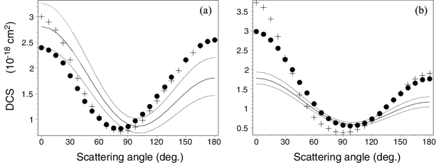
Figure 2: DCS for the pure $X\,^{1}\Sigma_{g}^{+}\rightarrow a\,^{3}\Sigma_{g}^{+}$ transition $\hbox{H}_{2}$ by electron impact at (a) 15 eV and (b) 18 eV. Solid lines, presents our calculation for $b=1.35$ (lower line), 1.40 (midline), and 1.45 (upper line); full circles, SMC results of Lima, et al. [17]; crosses, MCF results of Lee, et al. [18]

We think that possibilities of the ZRP methods allow to improve the results if

1) to use better approximations for a potential well in which the molecule oscillates,

2) to incorporate a separable potential into the theory (e.g., [2, 16]),

3) account other channels of electron excitations.

All these developments of the model could diminish the difference between the plots obtained by this approach, simulations ”ab initio” and experiments.

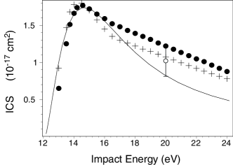
Figure 3: ICS for the pure $X\,^{1}\Sigma_{g}^{+}\rightarrow a\,^{3}\Sigma_{g}^{+}$ electron transition by electron impact in the 12-24 eV range. Solid line, present our calculation; full circles, SMC results of Lima, et al. [17]; crosses, MCF results of Lee, et al. An experimental point is also shown. [18]

.

5 Conclusion

We claim that the next step of our work is to unify both multichannel and higher partial modes [2] descriptions. This way we evaluate amplitudes of the $N_{2}$ electron-molecular scattering at low energies to fit recent experiments [19]. The results will be published elsewhere. The approach has one more natural generalization for multicenter scattering [5, 20]

6 Acknowledgements

We acknowledge consultations and priceless advices of V. Ostrovsky and I. Yurova and discussions with J. Sienkiewicz and M. Zubek.

Appendix A The vibrational harmonics $X_{nv}(R)$

In this work we approximate the theoretical energy ”curves” of molecular states by the Morse potentials

$$U_{n}(R)=\frac{\omega_{n}^{2}}{4\ae_{n}}\left[1-\exp\left(\displaystyle-2\sqrt{2\mu\ae_{n}}(R-R_{n})\right)\right]^{2}+U_{n},$$

where $\mu$ is reduced mass of molecule, $\omega_{n},\ae_{n}$ - corresponding vibration quantum and anharmonicity constant of the electronic state $n$, $U_{n}$ are energies at equilibrium internuclear distances $2R_{n}$, and $2R$ - internuclear distance. The choice arbitrariness of the parameters $U_{n}$ can be restricted by ground state energy fixation. For that we demand ground state energy be equal zero. In this case

$$U_{0}=-\frac{\displaystyle\omega_{0}}{\displaystyle 2}+\frac{\displaystyle\ae_{0}}{\displaystyle 4}.$$

The vibration harmonic $X_{nv}(R)$ satisfied the radial Schrödinger equation

$$-\frac{1}{8\mu}X^{\prime\prime}_{nv}+U_{n}(R)X_{nv}=E_{nv}X_{nv},$$

here argument $R$ is omitted. The physically reasonable solution of this equation can be expressed via orthogonal Laguerre polynomials $L_{v}^{\xi}(z)$

$$X_{nv}(R)=(C_{nv})^{-1/2}\,z^{\xi/2}\,\exp(-z/2)\,L_{v}^{\xi}(z),$$

where we use the following notation

$$z=\frac{\omega_{n}}{\ae_{n}}\,\exp(-2\sqrt{2\mu\ae_{n}}(R-R_{n})),$$

$$\hskip 28.45274pt\xi=\frac{\omega_{n}}{\ae_{n}}-2v-1.$$

The normalization factors $C_{nv}$ are defined by the normality condition. If functions $X_{nv}(R)$ are normalized to unity then the high accurate approximations for normalization factors are given

$$C_{nv}=\frac{\Gamma(\xi+v+1)}{\displaystyle v!\,\xi\sqrt{8m\ae_{n}\mathstrut}}.$$

The energy levels $E_{nv}$ constitute the finite sequence

$$E_{nv}=\omega_{n}\left(v+\frac{1}{2}\right)-\ae_{n}\left(v+\frac{1}{2}\right)^{2}+U_{n},\hskip 42.67912ptv=0,1,..,v_{m}.$$

References

• [1] Yu N Demkov and V N Ostrovsky, Zero-Range Potentials Method in Atomic Physics 1975 Leningrad: Leningrad State University (in Russian, English translation: Plenum, New York, 1988)
• [2] A S Baltenkov, Phys. Lett. A 286 (2000) 92-99.
• [3] E Fermi, Ric. Sci 7 (1936) 13.
• [4] G Breit, Phys. Rev. 71 (1947) 215.
• [5] Yu N Demkov and V S Rudakov, Zh. Eksp. Teor. Fiz. 1970 59 2035 [Sov. Phys.-JETP 1971 32 1103
• [6] Yu N Demkov, V N Ostrovsky, Zh. Eksp. Teor. Fiz. 1970 59 1765
• [7] G F Drukarev and I Yu Yurova, J. Phys. B: At. Mol. Phys. 1977 10 3551-8
• [8] G F Drukarev Adv. Quantum Chem. 1978 11 251
• [9] S Albeverio, F Gesztesy, R HΓΈegh-Krohn and H Holden Solvable Models in Quantum Mechanics 1988 (New York: Springer-Verlag)
• [10] N F Lane Rev. Mod. Phys. 1980 52 29-113
• [11] S I Drozdov Sov. Phys.-JETP 1955 1 591-2
• [12] D M Chase Phys. Rev. 1956 104 838-42
• [13] Yu D Oksyuk Sov. Phys.-JETP 1965 49 1261-73
• [14] V N Ostrovsky and V I Ustimov J. Phys. B: At. Mol. Phys. 1981 14 1139-56
• [15] D A Varshalovich, A N Moskalev and V K Khersonskii Quantum Theory of Angular Momentum 1975 Leningrad: Nauka (in Russian)
• [16] E de PrunelΓ© J. Phys. A (1997) 30 7831-7848
• [17] M A P Lima, T L Gibson, V McKoy, W M Huo, Phys. Rev. A (1988) 38 4527
• [18] M T Lee, M M Fujimoto, I Iga, J. Mol. Str. (1998) 432 197-209
• [19] M. Zubek, B. Mielewska, G. King J. Phys. B: At. Mol. Opt. Phys. 33 (2000) L527-L532.
• [20] R Szmytkowski and C Szmytkowski, J. Math. Chem. (1999) 26 243-254