Generation and control of resonance states in crossed magnetic and electric fields

Abstract

A two-dimensional electron system interacting with an impurity and placed in crossed magnetic and electric fields is under investigation. Since it is assumed that an impurity center interacts as an attractive $\delta$-like potential a renormalization procedure for the retarded Green’s function has to be carried out. For the vanishing electric field we obtain a close analytical expression for the Green’s function and we find one bound state localized between Landau levels. It is also shown by numerical investigations that switching on the electric field new long-living resonance states localized in the vicinity of Landau levels can be generated.

I Introduction

The quantum mechanical motion of electrons in two-dimensional space, subject to crossed magnetic and electric fields and in the presence of a single impurity described by a zero-range potential, provides a basis for the explanation of the integer quantum Hall effect P81 ; PJ82 ; JP84 ; PC91 ; CC98 ; GM99 ; HL99 . Until now in all considerations the electric field has been treated as a small perturbation. The purpose of the present work is to reconsider these investigations and to discuss some novel phenomena which appear for nonperturbative electric fields.

In our approach an attractive impurity is modelled as a zero-range potential center, as has been already exploited in PC91 ; CC98 . It turns out that in order to define such a point interaction one needs to renormalize the strength of the $\delta$-function and that such a renormalized potential is capable of supporting one localized state per Landau level. This finding also corresponds to the result obtained by Gyger and Martin GM99 . Investigating the case of a weak electric field they have proven that all localized states change into resonances with lifetimes varying with the electric field in a Gaussian way. With reference to these papers we shall focus our attention on the opposite regime, i.e., when the electric fields is strong. Our aim is to answer the following questions:

1. how many resonance states exist per one Landau level for a non-vanishing electric field?

2. what is a maximum electric field above which resonance states of a given lifetime cannot exist?

We shall see that apart from the well-known localized states lying between Landau levels PC91 ; CC98 ; GM99 new resonance states are created by a strong electric field, the lifetime of which can be comparable to or larger than typical times encountered in solid state physics.

Throughout this paper we use units in which $\hbar=1$.

II Attractive point interaction

The two-dimensional system we are concerned with is governed by the hamiltonian which, for convenience, we decompose into two parts, $H_{0}$ related to the physical situation for which the Green’s function is known and a $\delta$-like potential with the strength given by the so-called bare coupling constant $\lambda$,

$$H=H_{0}+\lambda\delta^{(2)}(\bm{r})\,.$$ (1)

Such a model has been extensively studied in the literature AGHH88 ; B75 ; FFR90 ; FFR91 ; MFSF00 ; W91 proving its usefulness in many branches of physics. It is, however, important to realize that the model is not free from difficulties. To be more precise, it exhibits divergencies which have to be tempered by renormalizing the bare coupling constant $\lambda$. Therefore, let us address this problem and show how to remove all divergent terms by considering the retarded Green’s function for the hamiltonian $H$.

Our starting point is the Lippmann-Schwinger equation which, in this particular case, adopts the form

$$G(\bm{r},\bm{r}^{\prime};E)=G_{0}^{(\mathrm{reg})}(\bm{r},\bm{r}^{\prime};E)$$

$$+\int\mathrm{d}^{2}\bm{r}^{\prime\prime}G_{0}^{(\mathrm{reg})}(\bm{r},\bm{r}^{\prime\prime};E)\lambda\delta^{(2)}(\bm{r}^{\prime\prime})G(\bm{r}^{\prime\prime},\bm{r}^{\prime};E)\,,$$ (2)

where the regularized Green’s function for the hamiltonian $H_{0}$, denoted by $G_{0}^{(\mathrm{reg})}(\bm{r},\bm{r}^{\prime};E)$, is assumed to be known. Now performing the foregoing integral over $\text{d}^{2}\bm{r}^{\prime\prime}$ and making some algebraic manipulations we arrive at the retarded Green’s function for our model

$$G(\bm{r},\bm{r}^{\prime};E)=G_{0}^{(\text{reg})}(\bm{r},\bm{r}^{\prime};E)$$

$$+\frac{G_{0}^{(\text{reg})}(\bm{r},\bm{0};E)G_{0}^{(\text{reg})}(\bm{0},\bm{r}^{\prime};E)}{\lambda^{-1}-G_{0}^{(\text{reg})}(\bm{0},\bm{0};E)}\,.$$ (3)

It appears that $G_{0}^{(\text{reg})}(\bm{0},\bm{0};E)$ is the only term which needs to be regularized in order to avoid divergencies. Let us explain how to cope with them analyzing the simplest case of a free electron with an effective mass $m^{*}$ interacting only with the $\delta$-like potential. In our approach we choose a particular regularization scheme which we call the proper time regularization. We expect that although the bare coupling constant $\lambda$ depends on the regularization scheme chosen, the observable quantities, like poles of the full Green’s function in the complex energy plane, cannot depend on this scheme. Indeed, we shall demonstrate that our method leads to the same equation for energies of localized states in the magnetic field as in CC98 .

For a free particle the retarded Green’s function in the so-called Fock-Schwinger proper time represantation IZ80 has the form

$$G_{0}^{(\text{reg})}(\bm{r},\bm{r}^{\prime};E)=-\text{i}\int_{-\text{i}\sigma}^{\infty}\text{d}t\text{e}^{\text{i}(E+\text{i}\varepsilon)t}$$

$$\int\frac{\text{d}^{2}\bm{k}}{(2\pi)^{2}}\exp\biggl{(}\text{i}\bm{k}\cdot(\bm{r}-\bm{r}^{\prime})-\text{i}\frac{\bm{k}^{2}}{2m^{*}}t\biggr{)}\,,$$ (4)

where the singularity for $\bm{r}=\bm{r}^{\prime}=\bm{0}$ is avoided by modifying the integration contour over the proper time $t$ in such a way that it lies just below the real axis (this means that $\sigma$ is a small positive parameter). Naturally, the retarded Green’s function for non-vanishing $\bm{r}$ or $\bm{r}^{\prime}$ is recovered by putting $\sigma=0$. Such a prescription we call the proper time regularization. Now, it is straightforward to show that the denominator in eq. (3) reads

$$D(E)=\lambda^{-1}+\frac{m^{*}}{2\pi}\int_{-\text{i}\sigma}^{\infty}\text{d}t\text{e}^{\text{i}(E+\text{i}\varepsilon)t}t^{-1}\,.$$ (5)

It is also clear that the integral above diverges logarithmically for small values of $t$ when $\sigma=0$. This divergence, however, can be absorbed into the bare coupling constant $\lambda$ giving the finite expression for the full Green’s function even for $\sigma$ equal to 0. Indeed, performing the proper time integration by parts we arrive at

$$D(E)=\lambda_{R}^{-1}+\frac{m^{*}}{2\pi}\biggl{(}\ln(\text{i})-\text{i}E\int_{0}^{\infty}\text{d}t\text{e}^{\text{i}(E+\text{i}\varepsilon)t}\ln(t/t_{0})\biggr{)}\,,$$ (6)

where $t_{0}$ is an arbitrary positive parameter of the same dimensionality as $t$, whereas $\lambda_{R}$ is the renormalized coupling constant defined by the relation

$$\lambda_{R}^{-1}=\lim_{\sigma\rightarrow 0}\Bigl{(}\lambda^{-1}-\frac{m^{*}}{2\pi}\ln\frac{\sigma}{t_{0}}\Bigr{)}\,.$$ (7)

Let us remark that in order to temper a singular part in the formula above the bare coupling constant $\lambda$ has to be negative. This means, in fact, that in two dimensions there cannot exist a repulsive point interaction. Having this in mind we shall restrict ourselves only to the case with an attractive point interaction for which, after performing the remaining integral, we have

$$D(E)=\lambda_{R}^{-1}+\frac{m^{*}}{2\pi}\ln\biggl{(}\frac{\text{e}^{-\gamma}}{-Et_{0}}\biggr{)}\,,$$ (8)

where $\gamma$ is the Euler’s constant. This equation shows that independently of numerical values of $\lambda_{R}$ and $t_{0}$ there exists $E$ such that the denominator of the full Green’s function vanishes, i.e., the two-dimensional zero-range potential always supports a bound state. Denoting the energy of this state by $E_{B}$ we end up with the following expression for the denominator $D(E)$,

$$D(E)=\frac{m^{*}}{2\pi}\ln\biggl{(}\frac{E_{B}}{E}\biggr{)}\,.$$ (9)

Let us add in closing that there still remains a free parameter of the theory, i.e., the energy of a bound state $E_{B}$. Nevertheless, it has now the clear physical meaning in the sense that its value can be measured, contrary to the artificial and physically unclear parameters $t_{0}$ and $\lambda_{R}$.

III Green’s function in external fields

In this section we consider the two-dimensional system composed of an electron and $\delta$-like impurity placed in the external magnetic and electric fields for which the hamiltonian $H_{0}$ can be written as

$$H_{0}=\frac{1}{2m^{*}}\Biggl{[}\Bigl{(}-\text{i}\partial_{x}+\frac{e\cal{B}}{2}y\Bigr{)}^{2}+\Bigl{(}-\text{i}\partial_{y}-\frac{e\cal{B}}{2}x\Bigr{)}^{2}\Biggr{]}-e{\cal E}x\,,$$ (10)

where the electric $\bm{\mathcal{E}}$ and magnetic $\bm{\mathcal{B}}$ fields are directed towards $x$ and $z$ axes, respectively, whereas the vector potential is taken in the circular gauge, $\bm{A}=\frac{1}{2}\bm{\mathcal{B}}\times\bm{r}$. As we have already pointed out, the problem of finding energies of impurity-induced resonance states consists in searching for zeros of the denominator in eq. (3). Therefore, what we have to know is the regularized Green’s function for the hamiltonian $H_{0}$. Applying the proper time regularization scheme discussed above we arrive at the regularized retarded Green’s function $G_{0}^{(\text{reg})}$,

$$G_{0}^{(\text{reg})}(\bm{r},\bm{r}^{\prime};E)=-\frac{m^{*}\omega}{4\pi}\int_{-\text{i}\sigma}^{\infty}\text{d}t\frac{\text{e}^{\text{i}(E+\text{i}\varepsilon)t}}{\sin\frac{\omega t}{2}}$$

$$\times\exp\Biggl{[}\frac{\text{i}m^{*}\omega}{4}\bigl{(}(x-x^{\prime})^{2}+(y-y^{\prime})^{2}\bigr{)}\cot\frac{\omega t}{2}$$

$$+\frac{\text{i}m^{*}\omega}{2}(xy^{\prime}-x^{\prime}y)+\frac{\text{i}e{\cal E}t}{2}(x+x^{\prime})$$

$$+\frac{\text{i}e\cal{E}}{\omega}\Bigl{(}\frac{\omega t}{2}\cot\frac{\omega t}{2}-1\Bigr{)}\Bigl{(}-y+y^{\prime}+\frac{e{\cal E}t}{2m^{*}\omega}\Bigr{)}\Biggr{]}\,,$$ (11)

and the denominator $D(E)$,

$$D(E)=\lambda^{-1}+\frac{m^{*}\omega}{4\pi}\int_{-\text{i}\sigma}^{\infty}\text{d}t\frac{\text{e}^{\text{i}(E+\text{i}\varepsilon)t}}{\sin\frac{\omega t}{2}}$$

$$\times\exp\Biggl{[}\frac{\text{i}t}{2m^{*}}\Bigl{(}\frac{e\cal{E}}{\omega}\Bigr{)}^{2}\Bigl{(}\frac{\omega t}{2}\cot\frac{\omega t}{2}-1\Bigr{)}\Biggl{]}\,,$$ (12)

where $\omega=|e|{\cal B}/m^{*}$ is the cyclotron frequency. Comparing this formula with eq. (5) one can notice that in both these expressions the integrals over $t$ diverge for small arguments exactly in the same way. Hence, we gather that now it is also possible to temper the divergent term by renormalizing the coupling constant $\lambda$. At this point let us introduce new dimensionless units. As a typical length scale for the problem we take $1/\sqrt{m^{*}\omega}$, whereas the dimensionless scaled electric field and energy are $\tilde{\cal E}=|e|{\cal E}/\sqrt{m^{*}\omega^{3}}$ and $\tilde{E}=2E/\omega$, respectively. Additionally, choosing a new variable $s=\omega t/2$ we find that

$$D(\tilde{E})=\frac{m^{*}}{2\pi}\Biggl{[}\ln\biggl{(}\frac{\tilde{E}_{B}}{\tilde{E}}\biggr{)}+\int_{0}^{\infty}\text{d}s\text{e}^{\text{i}(\tilde{E}+\text{i}\varepsilon)s}$$

$$\biggl{(}\frac{\exp\bigl{(}\text{i}{\tilde{\cal E}}^{2}s(s\cot s-1)\bigr{)}}{\sin s}-\frac{1}{s}\biggr{)}\Biggr{]}\,.$$ (13)

At first glance it might seem that the integral above is divergent for $s=n\pi$, where $n=1,2,..$. It is not, however, the case. Indeed, analyzing the integrand in the close vicinity of these points one can prove the convergence of the foregoing integral. Having this in mind we shall discuss below the special case when the electric field is switched off.

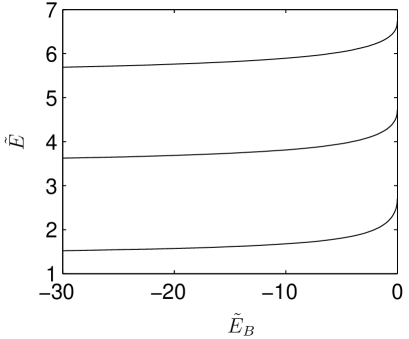
Figure 1: Impurity-induced localized states for the vanishing electric field

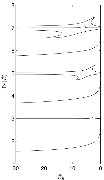
Figure 2: Real part of resonance states as the function of $\tilde{E}_{B}$ for $\text{Im}(\tilde{E})=10^{-4}$.

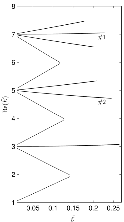
Figure 3: Real part of resonance states as the function of $\tilde{\cal{E}}$ for $\text{Im}(\tilde{E})=10^{-4}$.

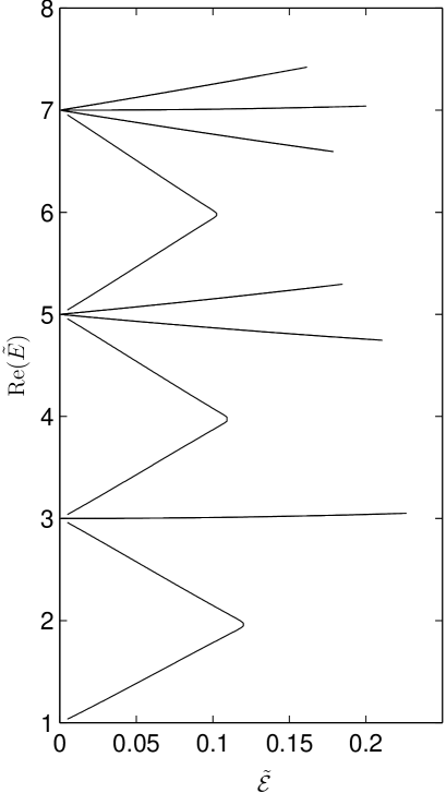
Figure 4: Real part of resonance states as the function of $\tilde{\cal{E}}$ for $\text{Im}(\tilde{E})=10^{-6}$.

IV Localized states in the external magnetic field

The problem without an electric field has been already examined by Cavalcanti and de Carvalho in CC98 . However, we have found it interesting to derive their equation for energies of the impurity-induced localized states using the proper time regularization scheme. Our point of departure is the function defined by eq. (13) with $\tilde{\cal E}=0$,

$$D(\tilde{E})=\frac{m^{*}}{2\pi}\Biggl{[}\ln\biggl{(}\frac{\tilde{E}_{B}}{\tilde{E}}\biggr{)}+\int_{0}^{\infty}\text{d}s\text{e}^{\text{i}(\tilde{E}+\text{i}\varepsilon)s}\biggl{(}\frac{1}{\sin s}-\frac{1}{s}\biggr{)}\Biggr{]}\,.$$ (14)

In order to treat these two integrals separately we regularize them first. This allows us to integrate them by parts and put finally the regularization parameter $\sigma$ equal to 0, keeping in mind, however, that the integration contour over $s$ lies just below the real axis,

$$D(\tilde{E})=\frac{m^{*}}{2\pi}\Biggl{[}\gamma+\ln(2\tilde{E}_{B})-\frac{\text{i}\pi}{2}$$

$$-\text{i}\tilde{E}\int_{0}^{\infty}\text{d}s\text{e}^{\text{i}(\tilde{E}+\text{i}\varepsilon)s}\ln\tan(s/2)\Biggr{]}\,.$$ (15)

Next, let us expand $\ln\tan(s/2)$ into series of $\text{e}^{-\text{i}s}$. This is allowed because the inequality $|\text{e}^{-\text{i}s}|<1$ holds for $s$ possessing a negative imaginary part, which is guaranteed by our choice of a regularization scheme. Hence, inserting into eq. (15) the series expansion

$$\ln\tan(s/2)=-\frac{\text{i}\pi}{2}-2\sum_{n=0}^{\infty}\frac{\text{e}^{-\text{i}(2n+1)s}}{2n+1}\,,$$ (16)

and carrying out all integrations term by term, we arrive at

$$D(\tilde{E})=\frac{m^{*}}{2\pi}\Biggl{[}\gamma+\ln(2\tilde{E}_{B})-\text{i}\pi$$

$$+2\tilde{E}\sum_{n=0}^{\infty}\frac{1}{(2n+1)(2n+1-\tilde{E})}\Biggr{]}\,.$$ (17)

Finally, relating the sum above to a digamma function $\psi(z)$, we find that the eigenenergies of our system are zeros of the following function

$$D(\tilde{E})=\frac{m^{*}}{2\pi}\Biggl{[}\ln\biggl{(}\frac{|\tilde{E}_{B}|}{2}\biggr{)}-\psi\biggl{(}\frac{1-\tilde{E}}{2}\biggr{)}\Biggr{]}\,,$$ (18)

which is adequate to the result derived in CC98 with the help of another regularization scheme. Zeros of $D(\tilde{E})$ determine the dependence of $\tilde{E}$ on $\tilde{E}_{B}$ for those localized states which are extracted from the Landau levels by the zero-range interaction. It is shown in Fig. 1 that only one state is extracted per Landau level, which is understandable, since in the degenerate Landau level there is only one state the wavefunction of which does not vanish at the origin, i.e., the cylindrically symmetric state BBCK . The situation changes if the electric field is present. It mixes this state with those Landau states which explicitly depend on the polar angle. For small electric fields such a mixing is also small and the effect of a point interaction can be neglected. However, for strong electric fields this effect becomes considerable as we are going to show this below.

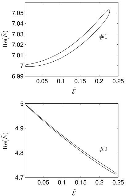
Figure 5: Two resonance states labeled by $\#1$ and $\#2$ in Fig. 3.

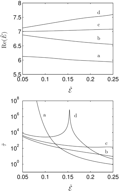
Figure 6: Real parts and lifetimes of some resonance states as the function of $\tilde{\cal E}$ for $\tilde{E}_{B}=-3$.

V Resonance states in external fields

In order to determine resonance energies for a non-vanishing electric field we have to find complex zeros of $D(\tilde{E})$ defined by eq. (13) and lying below the real axis. This means that we have to solve one complex equation, $D(\tilde{E})=0$, with four unknown real parameters: $\text{Re}(\tilde{E})$, $\text{Im}(\tilde{E})$, $\tilde{E}_{B}$ and the scaled electric field $\tilde{\cal{E}}$. To this end we shall fix one of these parameters, treat another one as a free parameter, and find the remaining two parameters by solving this equation, i.e., by determining poles of the full Green’s function. At the beginning let us fix the imaginary part of the resonance energy and find all possible zeros of $D(\tilde{E})$. The results are shown in Figs. 2 and 3. In Fig. 2 we present the real part, $\text{Re}(\tilde{E})$, of all resonance states of a given $\text{Im}(\tilde{E})=10^{-4}$ for the bound state energy $\tilde{E}_{B}$ between $-30$ and 0, as it has been already presented in Fig. 1 for the vanishing electric field (in both these figures we show only those states for which $\text{Re}(\tilde{E})>1$, i.e., lying above the first Landau level). We observe that, apart from the already existing impurity-induced bound states for $\tilde{\cal{E}}=0$, a non-vanishing electric field generates new resonance states which are located in the vicinity of Landau levels of energy $\hbar\omega(n+\frac{1}{2})$ for $n$ greater than 0. Moreover, as it follows from our numerical investigations, the number of these new resonance states is equal to $n$. This means that for a non-vanishing electric field and for a given quantum system, specified by the binding energy $\tilde{E}_{B}$, the number of impurity-induced resonances per Landau level is equal to $n+1$, where the quantum number $n$ labels the Landau energy. It appears that for the vanishing electric field real parts of energies of these new resonances approach the Landau energy, as it is shown in Fig. 3, in which we present the real part, $\text{Re}(\tilde{E})$, of all resonance states of a given $\text{Im}(\tilde{E})=10^{-4}$ as the function of $\tilde{\cal{E}}$. We observe that for a given imaginary part of resonances there is a maximum electric field above which no such resonance states exist. This is not a surprising fact. What is unexpected, however, is that the maximum electric field very little depends on the imaginary part of resonance energies chosen, as it is shown in Fig. 4 for $\text{Im}(\tilde{E})=10^{-6}$; although the lifetime of these new states has increased hundred times the maximum electric field has decreased only by a small fraction. This finding could suggest that even for nonperturbative electric fields there could exist long-living resonance states, as it will be discussed in details in KK2 .

The lines in Figs. 3 and 4 corresponding to the electric-field-induced resonances are, in fact, a narrow loops. In Fig. 5 we present in an enlarged scale two such resonances labelled by $\#1$ and $\#2$ in Fig. 3. It is clearly seen that for these particular resonances paths of the real part of resonance energies with a changing electric field represent closed loops which start from a Landau level. For a fixed electric field there are two states which correspond to two different binding energies $\tilde{E}_{B}$ and, as could be expected, the lower parts of these loops correspond to the stronger attraction, i.e., to the larger values of $|\tilde{E}_{B}|$.

Table 1: Physical values of the magnetic field $\cal{B}$, electric field $\cal{E}$ and lifetime $\tau$ for some chosen values of the bound state energy $E_{B}$ for a particular resonance.

$E_{B}$ [meV]	$B$ [T]	$\cal{E}$ [kV/m]	$\tau$ [ns]
1	0.506	6.423	7.52
2	1.013	18.167	3.76
4	2.025	51.383	1.88
6	3.038	94.396	1.25

In order to estimate the lifetime of one of these new resonance states let us take $\tilde{\cal{E}}=0.2647$ and $\tilde{E}_{B}=-2.2860459726451$ for which there exists the resonance of energy $\tilde{E}=3.0703456182811-10^{-4}\text{i}$. This resonance corresponds in Fig. 3 to the rightmost point lying near the first excited Landau level. In Table 1 we show some numerical values of the magnetic field $\cal{B}$ (in teslas), electric field $\cal{E}$ (in kilovolts per meter) and lifetime $\tau$ (in nanoseconds) for this resonance state and for some typical values of the binding energy $E_{B}$ of an electron with effective mass $m^{*}=0.067$ (in the electron’s mass unit) trapped by an attractive impurity in the GaAs quantum well PL90 . Our evaluations show that in spite of applying strong electric fields, which, in general, are expected to destabilize a system, one can observe generation of long-living states with lifetimes comparable to or even larger than typical timescales encountered in semiconductor heterostructures.

Let us close this paper discussing the resonances extracted by an attractive impurity and electric field from the third excited Landau level of $n=3$. We fix now the binding energy by assuming that $\tilde{E}_{B}=-3$ and draw the dependence of the complex resonance energy $\tilde{E}$ on the electric field intensity $\tilde{\cal{E}}$. As we have shown this above, the number of such states is equal to $n+1$ and $n$ of them approach the $n$-th Landau level for the vanishing electric field. The same conclusion can be reached looking at the upper panel of Fig. 6, while in the lower panel we present lifetimes of these states. We see that the state ’a’, related to the old states discussed before in P81 ; CC98 , is very stable for weak electric fields, but with an increasing $\tilde{\cal{E}}$ its lifetime suddenly decreases. On the contrary, the lifetimes of new electric-field-induced resonances, discussed in this paper, are shorter for weak fields, but with the increasing $\tilde{\cal{E}}$ we observe a peculiar behavior for one of them, i.e., for the resonance ’d’; instead of a continuous decrease we observe that for some particular values of $\tilde{\cal{E}}$ the lifetime increases, approaches its maximum value, and then starts decreasing. We call this phenomenon the electric-field-induced stabilization and we relate it to quantum vortices, positions of which are controlled by an electric field. A detailed analysis of this problem will be presented in our subsequent paper KK2 .

- (1) R. E. Prange, Phys. Rev. B 23 (1981) 4802.
- (2) R. E. Prange, R. Joynt, Phys. Rev. B 25 (1982) 2943.
- (3) R. Joynt, R. E. Prange, Phys. Rev. B 29 (1984) 3303.
- (4) F. Perez, F. A. B. Coutinho, Am. J. Phys. 59 (1991) 52.
- (5) R. M. Cavalcanti, C. A. A. de Carvalho, J. Phys. A 31 (1998) 2391.
- (6) S. Gyger, P. A. Martin, J. Math. Phys. 40 (1999) 3275.
- (7) E. H. Hauge, J. M. J. van Leeuwen, Physica A 268 (1999) 525.
- (8) S. Albeverio, F. Gesztesy, R. Høegh-Krohn, H. Holden, Solvable Models in Quantum Mechanics, Springer, Heidelberg, 1988.
- (9) I. J. Berson, J. Phys. B 8 (1975) 3078.
- (10) F. H. M. Faisal, P. Filipowicz, K. Rza̧żewski, Phys. Rev. A (1990) 6176.
- (11) P. Filipowicz, F. H. M. Faisal, K. Rza̧żewski, Phys. Rev. A (1991) 2210.
- (12) N. L. Manakov, M. V. Frolov, A. F. Starace, I. I. Fabrikant, J. Phys. B 33 (2000) R141.
- (13) K. Wódkiewicz, Phys. Rev. A 43 (1991) 68.
- (14) C. Itzykson, J. B. Zuber, Quantum Field Theory, McGraw-Hill, New York, 1980.
- (15) I. Białynicki-Birula, M. Cieplak, J. Kamiński, Theory of Quanta, Oxford University Press, New York, 1992.
- (16) K. Krajewska, J. Z. Kamiński, in preparation.
- (17) T. Pang, S. G. Louie, Phys. Rev. Lett. 65 (1990) 1635.