Preparation of spin squeezed atomic states by optical phase shift measurement

Abstract

In this paper we present a state vector analysis of the generation of atomic spin squeezing by measurement of an optical phase shift. The frequency resolution is improved when a spin squeezed sample is used for spectroscopy in place of an uncorrelated sample. When light is transmitted through an atomic sample some photons will be scattered out of the incident beam, and this has a destructive effect on the squeezing. We present quantitative studies for three limiting cases: the case of a sample of atoms of size smaller than the optical wavelength, the case of a large dilute sample and the case of a large dense sample.

1 Introduction

In an atomic sample the population of a state $|a\rangle$ can be measured non-destructively by a phase shift measurement of an optical field which acts on a transition from the state $|a\rangle$. If the field is not too close to resonance, it does not drive transitions out of the state $|a\rangle$, but an initial state vector of the sample with a binomial distribution of states with varying populations $n_{a}$ will be modified, and the quantum mechanical uncertainty of the number $n_{a}$ is reduced. This effect has been demonstrated experimentally [1, 2], and further experiments have shown [3], that two separate atomic ensembles can be driven into an entangled state by measurements of the total phaseshifts on an optical field passing through both samples.

A state preparation protocol that applies the outcome of quantum non-demolition (QND) measurements strongly relies on the fact that the measurement entails precisely the information that is applied in the changes of the state vector. When light interacts with atoms, apart from a phase shift of the incident field mode, also scattering out of the field mode occurs. The phase shift results from the interference between the incident field and the component of the scattered field in the incident mode, whereas scattering out of the incident mode is represented by components of the scattered wave function orthogonal to the incident wave function

The scattered photons carry information about the state of the atoms which is not recorded, and therefore the state of the system will in general not be the one deduced from the phase shift measurements alone, but rather an incoherent mixture of the states that one would have determined if also the scattered photons had been detetected.

The purpose of the present paper is to investigate the importance of photon scattering for the preparation of atomic states by phase shift measurements. In particular we shall derive criteria for the possibility to produce spin squeezed states.

The paper is organized as follows. In Sec. 2, we introduce the concept of spin squeezing and some useful relations for the mean values and variances of spin operators. In Sec. 3, we present our model for phaseshift measurements, and we introduce a formalism that makes it possible to take photon scattering into account. In Sec. 4, we analyze the information given by the registration of phase shifts only. In Sec. 5, we present simulations and analytical estimates valid for a cloud which is smaller than the optical wavelength, and for which photon scattering does not provide any information about the state of individual atoms. In Sec. 6, we consider the opposite case where the scattered photons can, in principle, be traced back to individual atoms in the cloud. In Sec. 7, we turn to the more complicated case of a large dense cloud, which turns out to present the most promising case for spin squeezing. Sec. 8 concludes the paper.

2 Collective spin representation of an atomic sample

The term spin squeezing originates in the treatment of two-level atoms as fictitious spin $\frac{1}{2}$ particles, $\vec{j}=\frac{1}{2}\vec{\sigma}$, where $\vec{\sigma}=(\sigma_{x},\sigma_{y},\sigma_{z})$ are the familiar $2\times 2$ Pauli matrices in the basis of atomic states $|a\rangle$ and $|b\rangle$. For a gas of $N_{at}$ atoms, the collective spin components

$$\vec{J}=\sum_{i}\vec{j}_{i}$$ (1)

have mean values which characterize the polarization and atomic state populations of the gas and quantum mechanical uncertainties which characterize the population statistics. For precision in spectroscopy and in atomic clocks it is pertinent to have a large mean spin vector of the sample and to have as small a variance as possible in a spin component orthogonal to the mean spin. Assume that the mean spin points in the $x$-direction. Heisenberg’s uncertainty relation states that

$$\Delta J_{y}\Delta J_{z}\geq\frac{1}{2}|\langle J_{x}\rangle|,$$ (2)

For the state with all atoms in their respective $j_{x}=\frac{1}{2}$ eigenstate, the binomial distribution leads to uncertainties of $\Delta J_{y}=\Delta J_{z}=\sqrt{N_{at}}/2$, in accord with the previous inequality. It was shown by Wineland et al [4], that if one can construct spin squeezed states which do not have the same uncertainty in the two spin components orthogonal to the mean spin, one may reduce the variance in a frequency measurement on $N_{at}$ particles by the factor

$$\xi^{2}=\frac{N_{at}(\Delta J_{z})^{2}}{\langle J_{x}\rangle^{2}}.$$ (3)

In [5] states were identified which for a given $\langle J_{x}\rangle$ have the smallest possible $\Delta J_{z}$. For large $N_{at}$ these are well represented by a Gaussian Ansatz for the amplitudes on states $|J=\frac{N_{at}}{2},M\rangle$ with different eigenvalues of $J_{z}$, in which case one obtains the approximate relation:

$$\langle J_{x}\rangle=(J+\frac{1}{2})(1-\frac{2(\Delta J_{z})^{2}}{(2J+1)^{2}})\exp(-\frac{1}{8(\Delta J_{z})^{2}})\sim J\exp(-\frac{1}{8(\Delta J_{z})^{2}}).$$ (4)

Spin squeezed states may be produced in a number of different ways: by absorption of squeezed light [6], by controlled collisional interaction in Bose-Einstein condensates [7] or in a classical gas [8], by coupling through a single motional degree of freedom or through an optical cavity field mode [9, 10]. One advantage of the QND scheme, analyzed in the present paper, is the automatic matching of the capability to produce the state and the ability to detect spin squeezing, which is done by the same kind of measurement. To verify that the fluctuations in $n_{a}$ have been reduced, one has to to show that two subsequent measurements agree (to within the desired uncertainty). If one can produce a state with reduced number fluctuations by means of a QND measurement, one will also have the resolving power to make use of such reduction in a high-precision experiment.

3 A physical setup for phase measurements.

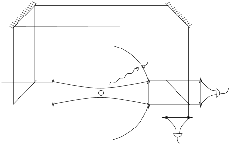
Figure 1: Configuration for a spin squeezing experiment. Atoms occupying a region in one arm of an interferometer are illuminated by a component of an optical field, incident from the left in the figure. The phase shift of the light field due to interaction with the atoms in a specific internal state is registered by the different photocurrents in the two detectors.

In Fig. 1, we illustrate a physical setup, where a beam of light enters a Stern-Gerlach interferometer which contains an atomic sample in one of its arms. By lenses, the field is focussed on the sample of transverse dimension $X$. For simplicity, we assume that the decomposition in plane waves of the incident photons is uniform for all angles $\theta$ smaller than the focussing angle $\theta_{0}$ which, in turn, is so small that the incident field is homogeneous across the area of the atomic cloud. Let $g_{0}=k\theta_{0}/(2\sqrt{\pi})$ denote the probability amplitude per unit surface for a photon to pass at the center of the mode ($g_{0}^{2}dxdy$ gives the probability that the photon passes in the area $dxdy$ around the center. A second lens maps the field back onto the inital mode, and the second beam splitter of the interferometer recombines the optical beams for read out of the phase shift induced by the presence of atoms in the lower part of the interferometer. The atoms populate states $|a\rangle$ and $|b\rangle$, and the optical field couples off-resonantly the state $|a\rangle$ to an auxiliary atomic state, so that a phase shift on the light field is induced which is proportional to the population $n_{a}$.

We now take into account the scattering of the photons by the atoms. The scattering is the normal spontaneous emission by the atom, given in the electric dipole approximation by well known angular distributions for photons of different polarization. Since our purpose is not to determine the angular distribution of scattered light, but rather to estimate its damaging effect on the atomic state preparation, we assume simply that every atom scatters photons isotropically with amplitude $f$. At low atomic saturation, the scattered photons are coherent with the incident field.

We shall present a calculation in which the photons are scattered one at a time by the sample. The scattered part of the wave function of a single photon is entangled with the state of the atomic sample, since an atomic state with a definite sequence of atoms populating the state $|a\rangle$, $\left|\vec{\epsilon}\right\rangle=\left|1:\epsilon_{1},2:\epsilon_{1},...,N_{\rm at}:\epsilon_{N_{\rm at}}\right\rangle$ where $\epsilon_{i}=\left|a\right\rangle$ or $\left|b\right\rangle$ leads to the photonic wave function

$$\psi_{{\rm scatt}_{\vec{\epsilon}}}=\frac{e^{ikr}}{r}f_{\vec{\epsilon}}(\Omega)g_{0}$$ (5)

where $f_{\vec{\epsilon}}(\Omega)$ depends on the state of the atomic sample.

In the first Born approximation, $f_{\vec{\epsilon}}(\Omega)$ is

$$f_{\vec{\epsilon}}(\Omega)=f\sum_{i,\epsilon_{i}=\left|a\right\rangle}e^{i\Delta\vec{k}.\vec{r_{i}}}\;,$$ (6)

where $\Delta\vec{k}$ is the difference between the scattered and the incident wave vectors. For $\theta<\theta_{0}$, $f_{\vec{\epsilon}}(\Omega)\simeq f_{\vec{\epsilon}}(0)=fn_{a}$.

In the Born approximation, the flux of photons is not conserved. To remedy this problem, we write the angular part of the photon wave function far from the atomic sample (sum of the scattered wave function and of the incident wave function) in the following form which is equivalent to the first order Born approximation but which conserves the photon flux.

$$f_{\vec{\epsilon}}(\Omega)=\left\{\begin{array}[]{l}f_{\vec{\epsilon}}(\Omega)g_{0}\mbox{ for }\theta>\theta_{0}\\ -i\frac{k}{2\pi g_{0}}\sqrt{(1-\sigma_{scatt})}\;\;e^{i\frac{2\pi}{k}fn_{a}|g_{0}|^{2}}\mbox{ for}\ \ \theta<\theta_{0}\end{array}\right.,$$ (7)

where

$$\sigma_{scatt}=\int_{\theta>\theta_{0}}\left|f_{\vec{\epsilon}}(\Omega)g_{0}\right|^{2}d\Omega$$ (8)

and $f_{\vec{\epsilon}}$ is given by Eq.(6).

If the atomic sample is in one of the states $\left|\vec{\epsilon}\right\rangle$, this state is unchanged by the transmission of a photon through the interferometer. The scattering state of the photon, however, depends, on the argument $\vec{\epsilon}$, and taking into account the unscattered component in the upper arm, we write this state in quantum notation as

$$\left|\psi\right\rangle_{p,\vec{\epsilon}}=\frac{1}{\sqrt{2}}\left(\left|\psi\right\rangle_{\rm ref}+\left|\psi\right\rangle_{\vec{\epsilon}}\right).$$ (9)

If the initial state of the cloud is in a superposition of different states $\left|\vec{\epsilon}\right\rangle$ the joint state of the photon and the atoms becomes the entangled state

$$\left|\Psi\right\rangle=\sum_{\vec{\epsilon}}C_{\vec{\epsilon}}\left|\psi\right\rangle_{p,\vec{\epsilon}}\left|\vec{\epsilon}\right\rangle=\sum_{\vec{\epsilon}}C_{\vec{\epsilon}}\frac{1}{\sqrt{2}}\left(\left|\psi\right\rangle_{\rm ref}+\left|\psi\right\rangle_{\vec{\epsilon}}\right)\left|\vec{\epsilon}\right\rangle.$$ (10)

It is at this stage, that the photodetection takes place. The photodetector 1 (resp. 2) of hte interferometer detects photons in the mode $\left|1\right\rangle=(e^{i\phi}\left|\psi\right\rangle_{\rm ref}+e^{-i\phi}\left|\psi\right\rangle_{\rm inc})/\sqrt{2}$ (resp. $\left|2\right\rangle=(e^{i\phi}\left|\psi\right\rangle_{\rm ref}-e^{-i\phi}\left|\psi\right\rangle_{\rm inc})/\sqrt{2}$), with $\left|\psi\right\rangle_{\rm inc}$ the field transmitted by the lower path of the interferometer in the absence of atoms. The detection of a photon in one of the detectors sketched in Fig.1 thus extracts the corresponding projection of the state vector $\left|\Psi\right\rangle$. This projection causes a non-continuous change of the atomic state vector amplitudes,

$$\begin{array}[]{l}C_{\vec{\epsilon}}\rightarrow\frac{1}{2}\left(e^{i\phi}+e^{-i\phi}\sqrt{(1-\sigma_{scatt})}\;\;e^{i\frac{2\pi}{k}fn_{a}|g_{0}|^{2}}\right)C_{\vec{\epsilon}},\ \ \mbox{detection 1,}\\ C_{\vec{\epsilon}}\rightarrow\frac{1}{2}\left(e^{i\phi}-e^{-i\phi}\sqrt{(1-\sigma_{scatt})}\;\;e^{i\frac{2\pi}{k}fn_{a}|g_{0}|^{2}}\right)C_{\vec{\epsilon}},\ \ \mbox{detection 2.}\\ \end{array}$$ (11)

We recall that $n_{a}$ and $\sigma_{scatt}$ depend on $\vec{\epsilon}$.

The probabilities, $\pi_{1}$ and $\pi_{2}$, to detect the photon in detector modes 1 and 2 are given by the squared norms of the vectors described by the new amplitudes after application of either projection according to (11). One may thus simulate the detection process by chosing one of the two prescriptions, update the amplitudes and renormalize the state vector. Detection of many photons is simulated by iterative updating of the state vector amplitudes.

In addition to the detection events just described, we have identified the possibility for photons to be scattered into other directions $\Omega$. The effect of such an event is of precisely the same character as the projections just described. If the photon is detected in the direction $\Omega$, the corresponding projection operator amounts to multiplying each amplitude of the initial atomic state with the corresponding scattering amplitude

$$C_{\vec{\epsilon}}\rightarrow f_{\vec{\epsilon}}(\Omega)C_{\vec{\epsilon}},\ \ \mbox{detection in direction}\ \Omega.$$ (12)

The detector actually has a finite size and detects the photon in a mode with $f$ centered around $\Omega$ but spread over $\delta\Omega$. With $\delta\Omega\ll 1/kX$, the scattered wave function is constant over $\delta\Omega$ and the probability to detect a scattered photon within the solid angle $\delta\Omega$ in the direction $\Omega$ is thus

$$P(\Omega)=\sum_{\epsilon}1/2|g_{0}|^{2}|f(\Omega)|^{2}|C_{\epsilon}|^{2}\delta\Omega$$ (13)

and the corresponding change of atomic state vector amplitudes given by (12).

To simulate the scattering of photons we divide the surface of the scattering sphere in sections by longitudes and lattitudes, and we imagine detectors located in each section. The poles of the sphere are in the direction of the incident beam and the solid angle delimited by $\theta<\theta_{0}$ correponding to the incident beam is of course not covered by such detectors since photons emitted in this solid angle go in the interferometer. For each incident photon, the probability to have a click in each detector of the sphere is computed. By adding the probabilities we compute $\sigma_{scatt}$ and we determine the probabilities to detect the photon in the detectors 1 or 2. The detector in which the photon is detected is chosen randomly in the simulation accordingly to all the calculated probabilities, and the state of the atoms is modified according to (11) or (12).

4 Information given by the interferometer

We shall now analyze the states resulting from the interaction with the field and the detection of the photons. In this section we neglect photon scattering, and we study only the effect of photons measured in detectors 1 and 2. We thus assume that $\sigma_{\rm scatt}=0$, in which case we can rewrite the factors in (11), and obtain the state of the atoms after the detection of $N_{1}$ photons in 1 and $N_{p}-N_{1}$ photons in detector 2,

$$\left|\psi\right\rangle=\sum_{\vec{\epsilon}}C_{\vec{\epsilon}}\cos\left(\phi-\pi g_{0}^{2}\frac{f}{k}n_{a}\right)^{N_{1}}\sin\left(\phi-\pi g_{0}^{2}\frac{f}{k}n_{a}\right)^{N_{p}-N_{1}}|\vec{\epsilon}\rangle.$$ (14)

In this equation we have ignored a phase factor $e^{i\pi fn_{a}g_{0}^{2}N_{p}/k}$, which corresponds to a phase shift of the state $\left|a\right\rangle$ or a rotation around $z$ in the spin language. To avoid such a rotation, one may apply an energy shift on state $|a\rangle$ or an alternative measurement scheme, where atoms in state $|b\rangle$ are also detected by optical phase shifts.

As a consequence of the photodetections, the populations of states with a definite number $n_{a}$ of atoms in state $|a\rangle$ are thus multiplied by the factors

$${\cal F}_{N_{p}}(N_{1},n_{a})=\cos\left(\phi-\pi g_{0}^{2}\frac{f}{k}n_{a}\right)^{2N_{1}}\sin\left(\phi-\pi g_{0}^{2}\frac{f}{k}n_{a}\right)^{2(N_{p}-N_{1})}.$$ (15)

By differentiation with respect to $n_{a}$, we find that ${\cal F}_{N_{p}}(N_{1},n_{a})$ is peaked at values $n_{a}^{0}$ which obey,

$$\tan(\phi+\pi g_{0}^{2}\frac{f}{k}n_{a}^{0})=\pm\sqrt{\frac{N_{p}-N_{1}}{N_{1}}}.$$ (16)

The values $n_{a}^{0}$ correspond of course to atomic populations so that the probability for the photons to be detected in modes $1$ and $2$ after the interaction are in agreement with the ratios $N_{1}/N_{p}$ and $N_{2}/N_{p}$ observed by the measurement.

To estimate the width of ${\cal F}_{N_{p}}(N_{1},n_{a})$, we calculate the second derivative of ${\cal F}_{N_{p}}(N_{1},n_{a})$ at $n_{a}^{0}$. We find that

$$\frac{\partial^{2}}{\partial{n_{a}}^{2}}{\cal F}_{N_{p}}(N_{1},n_{a})(n_{a}^{0})=-4N_{p}\left(\pi g_{0}^{2}\frac{f}{k}\right)^{2}{\cal F}_{N_{p}}(N_{1},n_{a}^{0}).$$ (17)

So, the more photons that are transmitted, the narrower is the width of the peaks in ${\cal F}_{N_{p}}(N_{1},n_{a})$. The width does not depend on the initial relative phase $\phi$ between the two arms of the interferometer or on the result of the measurement. If we suppose that ${\cal F}$ is gaussian, the following equation gives the rms width of ${\cal F}$ in $n_{a}$

$$\Delta n_{a_{\rm int}}=\frac{1}{2\pi g_{o}^{2}\frac{f}{k}\sqrt{N_{p}}}$$ (18)

The equation (16) has several solutions due to the two possible signs, and due to the periodicity of the $tan$-funtion. If several such solutions lie within the initial binomial distribution of $n_{a}$, the state obtained after the measurement will be a coherent superposition of spin states with different mean values of $J_{z}$, i.e., a kind of “Schrödinger cat”. However, a change of $N_{1}$ or $N_{p}-N_{1}$ by unity changes the relative phase between peaks by $\pi$. Thus, with realistic photon detectors with an efficiency smaller than unity, the relative phase is unknown and the system is described by a statistical mixture of the states.

In order to obtain spin squeezing, we want to ensure that only a single value of $n_{a}^{0}$ inside the initial distribution obeys Eq.(16), so that the detection unambiguosly leads to a more narrow distribution in $n_{a}$. This requires

$$\frac{\pi}{2\pi g_{0}^{2}f/k}>\sqrt{N}\;\mbox{ and }\;\frac{\Phi k}{\pi g_{0}^{2}f}\gg\sqrt{N}$$ (19)

Eq.(3) shows that it is not enough to reduce the uncertainty in $J_{z}$ to have useful spin squeezing, one must also ensure that the mean value of $J_{x}$ remains large. The outcome of the interferometric detection is close to ideal in this respect. The resulting state vector has amplitudes on the different $J_{z}$ eigenstates which follow a Gaussian distribution very well, and the approximation (4) for the mean spin is close to the maximum possible value for any given variance of $J_{z}$.

Using Eqs.(4,18) we obtain:

$$\xi=\frac{1}{\sqrt{N_{at}}\sqrt{N_{p}}\pi g_{0}^{2}\frac{f}{k}}e^{\pi^{2}g_{0}^{4}f^{2}N_{p}/2k^{2}}$$ (20)

The minimum value of $\xi$, for a fixed $N_{at}$, is

$$\xi_{\rm Min}=\sqrt{\frac{1}{N_{at}}}.$$ (21)

and is obtained for the photon number $N_{p}=k^{2}/\pi^{2}g_{0}^{4}f^{2}$. This value of $\xi$ is the minimum value allowed as shown in [4].

For a large number of atoms, the squeezing factor (21) can be really significant. The production of spin squeezed states by QND detection is susceptible, however, to two possible drawbacks caused by scattering of photons:

• scattered photons carry information about $J_{z}$, so that this quantity could in principle be known better than the width of ${\cal F}_{N_{p}}(N_{1},n_{a})$, and according to Eq.(4), the mean spin will be reduced

• scattered photons carry information about the spatial distribution of atoms in the state $\left|a\right\rangle$. The state is then no longer symmetric under exchange of the particles, $J$-values smaller than $N_{at}/2$ become populated, and the mean spin is accordingly reduced.

We shall now turn to a quantitative analysis of these effects.

5 Small cloud

In this section we consider the case of a cloud of atoms confined to a region in space smaller than the optical wavelength. This implies that the scattered photons will not contain information about the individual atoms in the ensemble. They will, however, carry information about $n_{a}$ that is not known to the experimentalist who measures only the fields by the detectors 1 and 2.

5.1 Numerical simulations

In a numerical simulation of the detection process we place atoms randomly in space according to a gaussian probability distribution, and we assume an initial state where all atoms are in $(\left|a\right\rangle+\left|b\right\rangle)/\sqrt{2}$. No restriction is made on the state at later times, which is expanded on the whole space of dimension $2^{N_{at}}$.

Figure 2: Results of a single simulation with 8 atoms whose spatial positions follow a gaussian law with a width of $10^{-2}\lambda/2\pi$. The angular spread of the incident beam is $\theta_{0}=0.45\pi$, close to the best that can be achieved. (a) Solid line : $\langle J_{z}\rangle$ as a function of the number of photons launched on the atoms. Long-dashed line : $\langle(J_{z}-\langle J_{z}\rangle)^{2}\rangle$. Short-dashed : Expected evolution of $\langle(J_{z}-\langle J_{z}\rangle)^{2}\rangle$ according to Eq.(18), taking into account the width of the initial distribution. (b) Evolution of $\langle\vec{J}^{2}\rangle$. The slight decrease shows that the state vector acquires only small components outside the symmetric subspace. (c) Evolution of the mean value of the spin in the horizontal direction (upper trace) and of the component of the spin along the expected direction (lower trace).

Fig.2 presents the evolution obtained for one particular history for a cloud of 8 atoms confined to a spatial region of dimension $\lambda/100$ and interrogated by a beam which is focussed on the atoms with an angular aperture of $\theta_{0}=0.45\pi$. The variance of the distribution of atoms in $\left|a\right\rangle$ (i.e., $\langle(J_{z}-\langle J_{z}\rangle)^{2}\rangle$) is plotted as well as the value expected from the results of section 4 (i.e., the multiplication of the initial distribution with the function ${\cal F}_{N_{p}}(N_{1},n_{a})$).

The value of $\langle\vec{J}^{2}\rangle$ keeps almost the initial maximal value of $20$ which indicates that the cloud stays in a symmetric state. This is expected as the atoms are closer to each other than $\lambda$ and then it is not possible to discriminate between the atoms with the scattered photons.

The last graph plots the value of $\langle J_{x}\rangle$ and of $\sqrt{\langle J_{x}\rangle^{2}+\langle J_{y}\rangle^{2}}$ which is the length of the mean spin in the horizontal plane, and which may be larger than the $x$-component because of small angular spin rotations that occur during photon scattering.

Figure 3: Average over 90 histories. (a) Thin solid line: evolution of $\langle(J_{z}-\langle J_{z}\rangle)^{2}\rangle$ as a function of the number of photons launched on the atoms. Note that this quantity is not measurable as $\langle J_{z}\rangle$ depends on the particular history. The dashed thin line gives the value expected from the scattering process only. It is a convolution between the initial distribution and a distribution of width given by Eq.(25), both assumed to be gaussian. Solid fat line: evolution of $\langle(J_{z}-J_{z_{calc}})^{2}\rangle$ where $J_{z_{calc}}$ is deduced, for each history, from Eq.(16) and from the knowledge of the number $N_{1}$ of photons detected in 1 and the number $N_{2}$ of photons detected in 2. This quantity agrees with Eq.(18) shown by the dashed fat line. (b) Solid line and short dashed line : Evolution of $\sqrt{\langle J_{x}\rangle^{2}+\langle J_{y}\rangle^{2}}$ and $\langle J_{x}\rangle$. A rotation of $\pi/kfg_{0}^{2}N_{photons}$ is applied in the $xy$-plane to compensate for the light shift. Dashed line : expected behavior due to the squeezing realized by scattering. Dotted line : expected behavior if the width of the $J_{z}$ distribution were only given by the interference detection.

Figure 3 shows the variance of $J_{z}$ and the mean value of $J_{x}$ and of the largest projection of the spin orthogonal to the $z$-axis. These results are obtained as the average over 90 independent realizations of our simulation. Both in Fig.2., and in Fig.3, we observe that the actual width in $J_{z}$ is smaller than the one concluded from the interferometric measurement : the fact that the atoms are coupled to other modes of the field also leads to squeezing. We recall, however, that the quantity $\langle(J_{z}-\langle J_{z}\rangle)^{2}\rangle$ is not a measurable quantity as $\langle J_{z}\rangle$ depends on the particular history. To exploit the squeezing due to scattering, one has to deduce $\langle J_{z}\rangle$ for each experiment by keeping track of the scattered photons.

5.2 Analytical estimates

The effect of the scattered photons can be computed analytically. Taking $\vec{r}_{i}=\vec{0}$ for all $i$, Eq.(6) and Eq.(12) show that the atomic state vector amplitudes are multiplied simply by the coefficient $\sqrt{\sigma_{1}}n_{a}$ after the detection of a scattered photon, and by the coefficient $\sqrt{1-\sigma_{1}}n_{a}$ in the absense of scattering where $\sigma_{1}=f^{2}g_{0}^{2}2\pi(1+\cos\theta_{0})$ is the scattering probability per atom in state $|a\rangle$.

After the detection of $N_{\rm scatt}$ out of a total number of $N_{p}$ photons, the wave function of the atoms becomes

$$\left|\psi\right\rangle=\sum_{n_{a}}C_{n_{a}}\left(\sqrt{\sigma_{1}}n_{a}\right)^{N_{\rm scatt}}\sqrt{1-\sigma_{1}n_{a}^{2}}^{N_{p}-N_{\rm scatt}}|\vec{\epsilon}\rangle,$$ (22)

so the probability distribution for $n_{a}$ is multiplied by

$${\cal G}(N_{\rm scatt},na)=(\sigma_{1}n_{a}^{2})^{N_{\rm scatt}}\left(1-\sigma_{1}n_{a}^{2}\right)^{N_{p}-N_{\rm scatt}}$$ (23)

This function is maximum on

$$n_{a_{0_{\rm scat}}}=\sqrt{\frac{N_{\rm scatt}}{2\pi(1+\cos\theta_{0})g_{0}^{2}f^{2}N_{p}}}$$ (24)

and its width can be estimated by assuming a gaussian shape with the same second derivative at the peak value

$$\Delta{n_{a}}_{\rm scat}\simeq\frac{1}{\sqrt{8\pi(1+\cos\theta_{0})g_{0}^{2}f^{2}N_{p}}}.$$ (25)

This width is always smaller than the width in $n_{a}$ of the function $\cal{F}$ because $g_{0}=k\theta_{0}/(2\sqrt{\pi})$, which is about the inverse of the transverse size of the beam on the cloud is always smaller than $k$,

$$\frac{\Delta{n_{a}}_{\rm scat}}{\Delta{n_{a}}_{\rm int}}=\frac{1}{4}\frac{g_{0}}{k}\frac{1}{1+\cos(\theta_{0})}<1$$ (26)

In every single realization, the width of the $n_{a}$ distribution is thus set by the number of scattered photons. After averaging over the unkown number of scattered photons we recover the broader distribution determined by the interferometer readout $N_{1}$ and $N_{2}$. Since the scattered photons do not drive atoms out of or into the state $|a\rangle$, the atomic density matrix obtained by an average over the number of scattered photons has the same diagonal elements in the basis $\{\left|J,M\right\rangle\}$ as the pure state that one would expect without photon scattering. But, the coherence terms of the density matrix are different from that of the pure state, and therefore the length of the mean spin will be altered by the scattering events. This is seen in Fig.3 b), where the three lower curves show the actual value of $\langle J_{x}\rangle$, of $\sqrt{\langle J_{x}\rangle^{2}+\langle J_{y}\rangle^{2}}$ and of the estimate (4), based on the small variance of $J_{z}$ due to the scattering. There is excellent agreement between these curves. The upper curve shows the larger value of the mean spin, that one would have obtained in the absence of scattering.

Our numerical simulations and our analytical estimates show that the effect of the scattering is to produce stronger squeezing than the interference measurement. After averaging over the unresolved scattering histories this squeezing does not affect the $n_{a}$ populations. But, its effect is to reduce the mean spin $\langle J_{x}\rangle$. In principle one could determine the number of scattered photons by the difference betwen the number of incident photons and the number of photons detected in the interferometer. For a poissonian source of light, however, this number cannot be determined to a higher precision than $\sqrt{N_{p}}$, which turns out to be larger than the required precision on the loss in photon number due to scattering.

As pointed out in section 2, the pertinent factor for spin squeezing is $\xi$ defined in Eq.(3). Using Eq. (18) for $\Delta J_{z}$ and Eqs.(4,25) to determine $\langle J_{x}\rangle$, we obtain

$$\xi=\frac{1}{\sqrt{N_{at}}\sqrt{N_{p}}\pi g_{0}^{2}\frac{f}{k}}e^{2\pi g_{0}^{2}f^{2}N_{p}}$$ (27)

The minimum value of $\xi$, for a fixed $N_{at}$, is

$$\xi_{\rm Min}=\sqrt{\frac{4e}{\pi N_{at}}}\frac{k}{g_{0}}.$$ (28)

and is obtained for the photon number $N_{p}=1/(\sqrt{4\pi}g_{0}^{2}f^{2})$. Because the size of the incident beam is larger than the wave length, $g_{0}<k$ and $\xi_{\rm Min}$ is larger than in the ideal case (21).

6 Large dilute cloud.

The effect of the scattering in the case of a cloud of extension larger than $\lambda$ is very different from the case of a small cloud. The number of scattered photons will still, as in the case of a small cloud, give us information on the total number of atoms in $\left|a\right\rangle$ and thus scattering will by itself produce squeezing. But in the case of a big cloud the angular distribution of the scattered photons gives also information on the position of the atoms in $\left|a\right\rangle$ and the atomic system therefore looses its invariance under permutation of the particles. The system will thus no longer be fully represented by the ($N_{at}+1$) Dicke states of maximal $J=N_{at}/2$. This does not affect the $z$ component of the spin but it strongly reduces the horizontal component of the spin.

6.1 Numerical simulation

In order to analyse the effect of the scattering alone, we have performed simulations of the evolution of the atomic state under detection of scattered photons. The directions of photodetection were chosen according to the procedure outlined in Sec. III, and Fig. 4 presents the result of a single simulation. In this simulation, we see a decrease of $\langle(J_{z}-\langle J_{z}\rangle)^{2}\rangle$ as well as a departure from the symmetric space (decrease of $\langle\vec{J}^{2}\rangle$). It is also clear that the decrease of $\langle(J_{z}-\langle J_{z}\rangle)^{2}\rangle$ is not as rapid as suggested by Eq.(25) which was valid for the small cloud.

Let us present a naive argument for the decrease of $\langle(J_{z}-\langle J_{z}\rangle)^{2}\rangle$: Assume that the cloud is in a state $\left|\vec{\epsilon}\right\rangle$ where each atom is either in $\left|a\right\rangle$ or $\left|b\right\rangle$. This state is unaffected by the interaction with the photon field. Let $p$ denote the probability that a photon is scattered by the cloud of atoms. In the absence of superradiance we expect $p=\sigma_{1}n_{a}$. The number of scattered photons $N_{scatt}$ thus has mean value $pN_{p}$ and uncertainty $\sqrt{pN_{p}}$, and we estimate $n_{a}$ by $N_{scatt}/\sigma N_{p}$ with an uncertainty of $\Delta n_{a}=\sqrt{n_{a}/\sigma N_{p}}$. If the state of the cloud expands over different $n_{a}$, the measurement of $N_{scatt}$ will reduce the width of the distribution by multiplying with a function of width $\Delta n_{a}=\sqrt{n_{a}/\sigma N_{p}}$. Taking $\sigma=4\pi g_{0}^{2}f^{2}$ and an initial state where all atoms are in $(\left|a\right\rangle+\left|b\right\rangle)/\sqrt{2}$

$$\langle(J_{z}-\langle J_{z}\rangle)^{2}\rangle=\frac{1}{\frac{4}{N_{at}}+\frac{8\pi g_{0}^{2}f^{2}N_{p}}{N_{at}}}$$ (29)

This function is plotted in Fig.4 (a). It reproduces quite well the numerical evolution, although the numerical evolution shows a faster squeezing.

After averaging over histories, as discussed in section 5, the squeezing due to scattering has no effect on the distribution of $n_{a}$ but it will reduce the horizontal component of the total spin. The upper dashed line in figure 4(c) predicts the reduction due to this effect, according to Eq.(4) taking $J=N_{at}/2$. We see that the horizontal spin determined in our simulation is even smaller than this estimate. The reason for this is that the state of the cloud is not in the symmetric subspace as assumed when we put $J=N_{at}/2$ in Eq.(4). The state of the cloud may be expanded on subspaces with different total $J$, and the mean value of $J_{x}$ is averaged over these different subspace components. To check the consistency of this picture we compare the decrease of $\langle\vec{J}^{2}\rangle$ with that of $\langle J_{x}\rangle$. The maximum $\langle J\rangle$ for a given$\langle\vec{J}^{2}\rangle=\langle J(J+1)\rangle$ is $\sqrt{1+4\langle J(J+1)\rangle}/2-1/2$ and it is obtained if only the subspace with $J=\langle J\rangle$ is populated. If we assume that the $J_{z}$ distribution (centered around zero) is the same in all subspaces we estimate that

$$\langle J_{x}\rangle\leq e^{-\frac{1}{8\mbox{Var}J_{z}}}\left(-\frac{1}{2}+\frac{\sqrt{1+4\langle J(J+1)\rangle}}{2}\right)$$ (30)

The curve corresponding to the right-hand side of this inequality is plotted in Fig.4. It reproduces quite well the decrease of $\langle J_{x}\rangle$.

Figure 4: The cloud contains 8 atoms spatially distributed according to a 3D gaussian probability law of rms width $10\lambda/2\pi$. The incident beam, focussed on the atoms, has an angular spread $\theta_{0}=2\sqrt{\pi}g_{0}/k=2\sqrt{\pi}*0.05=0.14$. (a) : Evolution of $\langle J_{z}\rangle$ (solid line) and $\langle(J_{z}-\langle J_{z}\rangle)^{2}\rangle$ (long dashed line) as functions of the number of photons which are launched on the atoms. The dotted line indicates the value of $\langle(J_{z}-\langle J_{z}\rangle)^{2}\rangle$ expected for a dense cloud of 8 atoms illuminated by the same beam (Eq. (25)). The short dashed line gives the result of Eq.(29). (b) : Evolution of $\langle\vec{J}^{2}\rangle$. The first drop from the maximal value 20 occurs at the first detection of a scattered photon. (c) : Evolution of the mean horizontal spin (solid line). In dashed lines is shown the expected value of $\langle J_{x}\rangle$ according to Eq.(4) for $J=N_{at}/2$. The result of Eq. (30) is shown with the short-dashed line.

6.2 Analytical estimates

If the atomic cloud is dilute enough and not too large it is possible to know by which atom any photon has been emitted. In other words, it is possible to design an optical system which collects all the photons emitted outside the incident mode and which produces a separate image of each atom. This implies that the flux of scattered photons is only proportional to $n_{a}$ and not to $n_{a}^{2}$: there is no superradiance. Then the scattered photons give information on the total number of atoms in $\left|a\right\rangle$ but also on which atoms are in $\left|a\right\rangle$. The second effect damages the squeezing realised by the interference measurement as it decreases correlations between atoms. When a photon is transmitted, the probability that it is scattered by an atom in $\left|a\right\rangle$ is approximately $4\pi g_{0}^{2}f^{2}$. Thus after about $N_{p}=1/4\pi g_{0}^{2}f^{2}$ photons have been transmitted, we know almost with certainty if the atom is in $\left|b\right\rangle$ or $\left|a\right\rangle$, and there is then almost no correlation between the atoms and hence no squeezing. Indeed, as each atom is either in $\left|a\right\rangle$ or $\left|b\right\rangle$, $\langle j_{x}\rangle=0$ for each atom. In order to observe squeezing the number of photons used in the experiment is limited and this in turn limits the reduction in Var$(J_{z})$.

Within a more quantitative analysis of the effect of scattering let $\phi$ denote the flux of incident photons. As long as an atom scatters no photons, its state evolves according to the effective Hamiltonian

$$H_{nh}=-\frac{i}{2}\phi 4\pi g_{0}^{2}f^{2}\left|a\right\rangle\left\langle a\right|.$$ (31)

The probability to scatter a photon during $\delta t$ is

$$P\delta t=\left\langle a\right|\psi\left|a\right\rangle^{2}\phi 4\pi g_{0}^{2}f^{2}\delta t.$$ (32)

After averaging over histories only the coherence term $\sigma_{ab}$ of the density matrix evolves and it obeys

$$\frac{d\sigma_{ab}}{dt}=-\frac{\phi}{2}4\pi g_{0}^{2}f^{2}\sigma_{ab}.$$ (33)

Thus, $\langle j_{x}\rangle=1/2(\sigma_{ab}+\sigma_{ab}^{*})$ follows the same exponential decay, and it follows that the total spin $J_{x}=\sum j_{x_{i}}$ decreases as

$$\langle J_{x}\rangle_{t}=\langle J_{x}\rangle_{0}e^{-2\phi\pi g_{0}^{2}f^{2}t}=\langle J_{x}\rangle_{0}e^{-2N_{p}\pi g_{0}^{2}f^{2}}$$ (34)

The reduction of $\langle J_{x}\rangle$ due to the interferometric dectection, estimated using Eq.(4) is less important than the reduction of $\langle J_{x}\rangle$ due to scattering and we will neglect it here. Var$(J_{z})$ is given by Eq.(18), and the squeezing factor writes

$$\xi=\frac{1}{\sqrt{NN_{p}}\pi g_{0}^{2}\frac{f}{k}}e^{2N_{p}\pi g_{0}^{2}f^{2}}.$$ (35)

Its minimum value is

$$\xi_{\rm Min}=\sqrt{\frac{2e}{\pi N}}\frac{k}{g_{0}},$$ (36)

and it is obtained for $N_{p}=1/(4\pi g_{0}^{2}f^{2})$.

Although the physical regimes are very different, the result is similar to Eq.(26).

7 Large dense cloud

We now turn to an analysis of the situation of many atoms in a large cloud with a density which is large compared to $1/\lambda^{3}$. In this case, we are not able to carry out simulations, and we are therefore restricted to an analytical approach. We shall make the assumption of a dense cloud, so that it may be divided into a large number of cells of size $a^{3}$ smaller than $\lambda^{3}$ but still containing a large number of atoms. For simplicity, we assume that the distribution of atoms is uniform over a box of size $L_{x}=L_{y},L_{z}$. As the size of the cell is smaller than $\lambda^{3}$, the scattering of photons does not bring information on the repartitioning of the atoms in $\left|a\right\rangle$ inside each cell and the state of the cloud can be described by states that are symmetric under exchange of particles inside each cell. The states $\left|\vec{n}\right\rangle=\left|n_{1},n_{2},...,n_{M}\right\rangle$ with well defined number $n_{1}$, $n_{2}$,…,$n_{M}$ of atoms in $\left|a\right\rangle$ in the cells 1,2,…,M are not modified by the scattering. The number of atoms per cell is sufficiently large so that we consider that the number of atoms in $\left|a\right\rangle$, on the order of $N_{cell}/2$, can be considered as a continuous variable with fluctuations of order $\sqrt{N_{cell}}/2$.

7.1 Initial state of the cloud

Initially, all the atoms are in the state $1/\sqrt{2}(\left|a\right\rangle+\left|b\right\rangle)$. The expansion of the state of the cloud on the basis $\{\left|\vec{n}\right\rangle\}$ is then

$$\left|\psi\right\rangle_{at}=\int dn_{1}\int dn_{2}...\int dn_{M}c(n_{1})c(n_{2})...c(n_{M})\left|n_{1},n_{2},...,n_{M}\right\rangle$$ (37)

where $c(n)$ is the square root of the binomial distribution of mean value $N_{cell}/2$ which we will approximate by a gaussian distribution.

We will now define the new variables

$$\left\{\begin{array}[]{l}N_{c_{i_{x},i_{y},i_{z}}}=\sqrt{\frac{2}{M}}\sum_{\vec{l}}n_{\vec{l}}\cos(\vec{K}_{\vec{i}}.\vec{r}_{\vec{l}})\\ N_{s_{i_{x},i_{y},i_{z}}}=\sqrt{\frac{2}{M}}\sum_{\vec{l}}n_{\vec{l}}\sin(\vec{K}_{\vec{i}}.\vec{r}_{\vec{l}})\\ N_{0}=\sqrt{\frac{1}{M}}\sum_{\vec{l}}n_{\vec{l}}\end{array}\right.$$ (38)

with

$$\left\{\begin{array}[]{l}\vec{K}_{\vec{i}}=\frac{2\pi}{aN_{x}}i_{x}\vec{x}^{0}+\frac{2\pi}{aN_{y}}i_{y}\vec{y}^{0}+\frac{2\pi}{aN_{z}}i_{z}\vec{z}^{0}\\ \vec{r}_{\vec{l}}=al_{x}\vec{x}^{0}+al_{y}\vec{y}^{0}+al_{z}\vec{z}^{0}\end{array}\right.$$ (39)

where $i_{z}<0$ or ($i_{z}=0$ and $i_{x}<0$) or ($i_{z}=i_{x}=0$ and $i_{y}<0$).

Note that all the operators $N_{\alpha}$ and $N_{\beta}$ commute since they are all diagonal in the basis $\{\left|\vec{n}\right\rangle\}$.

The initial state of the cloud can be expanded on the new basis of eigenstates

$$\left|\psi\right\rangle_{at}=\begin{array}[t]{l}\int dN_{0}\int dN_{c_{1}}\int dN_{s_{1}}...\int dN_{c_{(M-1)/2}}\int dN_{s_{(M-1)/2}}\\ C(N_{0})h(N_{c_{1}})h(N_{s_{1}})...h(N_{c_{(M-1)/2}})h(N_{s_{(M-1)/2}})\left|N_{0},N_{c_{1}},N_{s_{1}},...,N_{c_{(M-1)/2}},N_{s_{(M-1)/2}}\right\rangle\end{array}$$ (40)

where $h$ is a gaussian centered on 0 with an rms width of $\sqrt{N_{cell}/2}$ ($h^{2}$ has a width $\sqrt{N_{cell}}/2$ equal to the width of $c^{2}(n_{i})$) and $C$ has the same width but is centered on $\sqrt{M}N_{cell}/2$. Initially, there is no correlation between the distributions in $N_{{s/c}_{i}}$ and they are all the same.

The vector space can be seen as a tensor product of (M+1)/2 spaces: The space acted upon by $N_{0}$, and for each $i$, the space ${\cal E}_{i}$ acted upon by the operators $N_{c_{i}}$ and $N_{s_{i}}$. All these spaces have infinite dimension and they admit as basis states $\left|N_{c_{i}},N_{s_{i}}\right\rangle$ where $N_{c_{i}},N_{s_{i}}$ are real. This basis will turn out to be useful for the description of the state vector dynamics due to photon scattering.

Figure 5: Inital distribution among the states ($\left|n_{1},n_{2},...,n_{M}\right\rangle$) or the states ($\left|N_{0},N_{c_{1}},N_{s_{1}},...,N_{c_{(M-1)/2}},N_{s_{(M-1)/2}}\right\rangle$) in the case where there are only three cells ($M=3$). Represented is a surface on which the population is constant. The circle surrounding the origin is the projection of the sphere on the $(N_{c},N_{s})$ plane.

7.2 Effect of the scattering

Due to energy and momentum conservation in the scattering process, a fluctuation in the cloud will couple to the light only if its Fourier transform has components $\vec{K}_{i}$ on the scattering sphere defined as the vectors $\vec{k}_{d}$ which fulfill $|\vec{k_{d}}-\vec{k}_{inc}|=k$.

We will now assume for simplicity that the Fourier transform associated with each $\vec{K}_{i}$ are uniform over disjoint volumes $\delta k_{x}=2\pi/L_{x}$, $\delta k_{y}=2\pi/L_{y}$ and $\delta k_{z}=2\pi/L_{z}$, shown as small rectangles in Fig. 6. The circle in Fig. 6 depicts the scattering sphere and crosses represent the dicrete $\vec{K}_{i}$ wave vectors which contribute to the scattering. With this approximation, the observation of a scattered photon gives information on the modulation of the atomic population in state $|a\rangle$ with the corresponding discrete wave vector.

Figure 6: Diffusion sphere and components of the discret Fourrier decomposition which participate to the diffusion

Let us consider a $\vec{K}_{i}$ which is on the scattering sphere and the associated solid angle $\delta\Omega_{i}$. The effect on the state of the system associated with the detection of a photon in this solid angle is given by the operator

$${\cal P}(\Omega)=\sqrt{\delta\Omega_{i}}g_{0}f\sum_{\vec{l}}n_{\vec{l}}e^{i(\vec{k_{d}}-\vec{k}_{inc})\vec{r}_{\vec{l}}}=\sqrt{\delta\Omega_{i}}g_{0}f\sqrt{\frac{M}{2}}(N_{c_{\vec{i}}}+iN_{s_{\vec{i}}}).$$ (41)

This operator changes the relative phase between the component with fluctuations in cosinus and sinus components. Because the operator in Eq.(40) acts only on the space ${\cal E}_{i}$, no correlations between fluctuations at different wave vector appear and the state of the cloud will thus stay on the form

$$\left|\psi_{0}\right\rangle\left|\psi_{1}\right\rangle...\left|\psi_{(M-1)/2}\right\rangle$$ (42)

where $\left|\psi_{i}\right\rangle$ is a state of the space ${\cal E}_{i}$. Note that this result is an approximation which relies on our assumption that the Fourier transform of the fluctuations at different $\vec{K}_{i}$ are disjoint. Furthermore, the assumption that atoms are uniformly distributed over our spatial grid is important. Indeed, if the number of atoms in $\left|a\right\rangle$ in different cells is not the same for each cell, the initial state would present correlations between $K_{i}$’s and knowledge about the state in the subspace ${\cal E}_{i}$ would also implies knowledge about the state in other ${\cal E}_{j}$.

If a photon is detected in the incident mode, the effect on the state of the atoms, to second order in $f$, is given by

$${\cal P}=\prod_{i}\sqrt{1-g_{0}^{2}f^{2}\frac{M}{2}\delta\Omega_{i}\left(N_{c_{i}}^{2}+N_{s_{i}}^{2}\right)}.$$ (43)

Thus, in this approximation, neither scattering nor absence of scattering yields correlations between different $K_{i}$’s, and the state of the cloud will stay in a product state as in Eq.(42).

After transmission of $N_{p}$ photons and the detection of $N_{sc}$ photons scattered in the direction $\vec{k}_{diff}=\vec{k}_{inc}-\vec{K}_{i}$, the wave function in the space ${\cal E}_{i}$ becomes

$$\left|\psi_{i}\right\rangle=\int dN_{c_{i}}\int dN_{s_{i}}\left(N_{c_{i}}+iN_{s_{i}}\right)^{N_{sc}}\left(\sqrt{1-g_{0}^{2}f^{2}\frac{M}{2}\delta\Omega_{i}\left(N_{c_{i}}^{2}+N_{s_{i}}^{2}\right)}\right)^{N_{p}-N_{sc}}h(N_{c_{i}})h(N_{s_{i}})\left|N_{c_{i}},N_{s_{i}}\right\rangle$$ (44)

Thus, the population of the states $\left|N_{c_{i}},N_{s_{i}}\right\rangle$ is multiplied by the factor

$${\cal G}(\sqrt{N_{c_{i}}^{2}+N_{s_{i}}^{2}})\begin{array}[]{l}=\left(N_{c_{i}}^{2}+N_{s_{i}}^{2}\right)^{N_{sc}}\left(1-g_{0}^{2}f^{2}\frac{M}{2}\delta\Omega_{i}\left(N_{c_{i}}^{2}+N_{s_{i}}^{2}\right)\right)^{N_{p}-N_{sc}},\end{array}$$ (45)

which depends only on $N_{c_{i}}^{2}+N_{s_{i}}^{2}$. This is expected as the detection of the scattered photons does not reveal any information about the phase of the spatial grating in the cloud of atoms in $\left|a\right\rangle$.

A calculation similar to the one in Sec. 6.2 shows that ${\cal G}$ has a width

$$\Delta N_{i}=\frac{1}{\sqrt{\delta\Omega_{i}\frac{M}{2}g_{0}^{2}f^{2}N_{p}}}.$$ (46)

Figure 7 depicts the final distribution over the states $N_{0},(N_{c_{i}},N_{s_{i}})$ in the simple case where the cloud is divided into only three cells.

Figure 7: Distribution over the states ($\left|n_{1},n_{2},...,n_{M}\right\rangle$) or the states ($\left|N_{0},N_{c_{1}},N_{s_{1}},...,N_{c_{(M-1)/2}},N_{s_{(M-1)/2}}\right\rangle$) after the measurement. Compare with Fig. 5. The case of only 3 cells is represented. the distribution of the population in the basis ($\left|N_{c},N_{s}\right\rangle$) for a well defined $N_{0}$ does not depend on $N_{0}$ and is given by the projection of the torus on the plane $(N_{c},N_{s})$.

7.3 Effect of scattering on $<J_{x}>$

Photons scattered in the forward direction in the solid angle $\theta<\theta_{0}$ give information on $N_{0}$ and thus on the total number of atoms in $\left|a\right\rangle$. The other scattered photons give information on the spatial fluctuations of the atoms in $\left|a\right\rangle$ and, in the case we consider where the number of atoms per cell is large and approximately constant, no information on $N_{0}$ is given by the photons scattered outside the solid angle $\theta<\theta_{0}$. This is completely different from the case considered in section 6.2 where in a single experiment the number of atoms in $\left|a\right\rangle$ was mainly determined by the scattering.

In the case considered here, even if $N_{0}$ is not affected by the scattering outside the incident beam, the state is affected by scattering events due to the departure from the space of states which is symmetric under exchange of atoms. After a series of detections, the state of the cloud has components in different subspaces $J$ because the scattering (or its absence) brings the system into non symmetric states with $J<N/2$. We thus expect $\langle J_{x}\rangle$ to be smaller than the value obtained for a state with the same distribution of $J_{z}$ eigenstates but in the symmetric subspace $J=N/2$.

We have

$$\langle J_{x}\rangle=\sum_{i}\langle J_{x_{i}}\rangle$$ (47)

where $\langle J_{x_{i}}\rangle$ is the mean value of $J_{x}$ corresponding to the atoms of the cell $i$. It is

$$\langle J_{x_{i}}\rangle=\int dn_{1}...dn_{i-1}dn_{i+1}...dn_{M}\left(\int dn_{i}|f(n_{1},...,n_{M})|^{2}\right)\langle J_{x_{i}}\rangle_{n1,...,n_{i-1},n_{i+1},...,n_{M}}$$ (48)

The state is invariant by exchange of atoms inside a single cell, and the results of Eq.(4) can be used to estimate $\langle J_{x_{i}}\rangle_{n1,...,n_{i-1},n_{i+1},...,n_{M}}$ by

$$\langle J_{x_{i}}\rangle_{n1,...,n_{i-1},n_{i+1},...,n_{K}}\simeq\frac{N_{cell}}{2}e^{-\frac{1}{8\rm{Var}(J_{z_{i}})}}$$ (49)

Taking $i=1$, we note that $\rm{Var}(J_{z_{1}})$ is the rms width of the function

$$F(n_{1})={\cal C}^{\prime}\left(\frac{n_{1}}{\sqrt{M}}+\frac{n_{2}+...+n_{M}}{\sqrt{M}}\right)\prod_{i}{\cal H}_{i}^{\prime}\left(\sqrt{N_{c_{i}}(n_{1})^{2}+N_{s_{i}}(n_{1})^{2}}\right)$$ (50)

where ${\cal C}^{\prime}(N_{0})$ is the final population distribution over the states $\{\left|N_{0}\right\rangle\}$ and ${\cal H}_{i}^{\prime}(N_{i})={\cal G}_{i}(N_{i})h^{4}(N_{i})$ is the final population distribution among the states $\{\left|N_{c_{i}}=\cos(\alpha)N_{i},N_{s_{i}}=\sin(\alpha)N_{i}\right\rangle\}$ (It does not depend on the angle $\alpha$).

For the initial distribution, ${\cal C}^{\prime}(n_{1}/\sqrt{M}+...)$ has an rms width of $\sqrt{MN_{cell}}/2$ in $n_{1}$ and ${\cal H}_{i}\left(\sqrt{N_{c_{i}}(n_{1})^{2}+N_{s_{i}}(n_{1})^{2}}\right)=h^{2}(\sqrt{2/M}\cos(\vec{K}_{i}.\vec{r}_{1})n_{1}+...)h^{2}(\sqrt{2/M}\sin(\vec{K}_{i}.\vec{r}_{1})n_{1}+...)$ has an rms width of $\sqrt{MN_{cell}/8}$ as a function of $n_{1}$. Thus, Eq.(50) gives an rms width $\Delta J_{z_{1}}$ equal to $\sqrt{N_{cell}}/2$ for any $(n_{2},...,n_{M})$, which is expected.

After the detection, the width of ${\cal C}^{\prime}$ has been reduced by the interference measurement to $\Delta n_{a_{inter}}/\sqrt{M}$ and the rms width in $n_{1}$ of ${\cal C}^{\prime}(n_{1}/\sqrt{M}+...)$ is

$${\Delta n_{1}}_{inter}=\Delta n_{a_{inter}}.$$ (51)

The detection of scattered photons modifies the distribution ${\cal H}_{i}^{\prime}$ which is then no longer separable in $N_{c_{i}}$ and $N_{s_{i}}$. But it follows from the definition (38) and from Eq.46 that, in average, ${\cal H}_{i}^{\prime}$ has an rms width in $n_{1}$ which scales as

$${\Delta n_{1}}_{i}\sim\sqrt{M}\Delta N_{i}$$ (52)

If we assume that the distribution of $n_{1}$ is given by the initial Gaussian, which is multiplied by gaussian factors due to the interferometric detection and due to the scattering, we obtain the result

$$\frac{1}{\Delta n_{1}^{2}}=\frac{1}{\Delta n_{a_{inter}}^{2}}+\sum_{i,\vec{K}_{i}\in S_{scatt}}\frac{1}{M\Delta N_{i}^{2}}+\sum_{i,\vec{K}_{i}\notin S_{scatt}}\frac{8}{MN_{cell}}$$ (53)

The squeezing due to scattering and due to interferometric detection is significant, and we can hence ignore the last term, which is due to the initial width of the distribution. The contribution due to the interferometric detection is given by Eq.(18), and the sum over the $i$ for which $\vec{K}_{i}$ is on the scattering sphere follows from Eq.(46):

$$\sum_{i,\vec{K}_{i}\in S_{scatt}}\frac{1}{M\Delta N_{i}^{2}}=2\pi g_{0}^{2}f^{2}N_{p}.$$ (54)

By comparison of Eq.(18) and (54), we see that the contribution due to interferometric detection is approximately a factor $g_{0}^{2}/k^{2}$ times the one due to scattering. $1/g_{0}^{2}$ is larger than the area of the cloud which itself is much larger than $\lambda^{2}$. Thus, $g_{0}^{2}/k^{2}\ll 1$ and the width in $n_{1}$ is mainly determined by the scattered photons :

$$\frac{1}{\Delta n_{1}^{2}}=\frac{1}{\rm{Var}J_{z_{1}}}\simeq\frac{1}{2}\sigma_{1}N_{p}.$$ (55)

Coming back to Eq.(49) and Eq.(47), we get

$$\langle J_{x}\rangle\simeq\frac{N}{2}e^{-\frac{\pi}{8}g_{0}^{2}f^{2}N_{p}}$$ (56)

Thus, the squeezing factor writes

$$\xi=\frac{1}{\sqrt{NN_{p}}\pi g_{0}^{2}\frac{f}{k}}e^{\frac{\pi}{8}g_{0}^{2}f^{2}N_{p}}$$ (57)

Its minimum value, achieved for $N_{p}=4/(\pi g_{0}^{2}f^{2})$, is

$$\xi_{Min}=\sqrt{\frac{e}{4\pi N_{at}}}\frac{k}{g_{0}},$$ (58)

which is similar to the result obtained for the small cloud and for the dilute sample.

8 Conclusion

We have presented an analysis of the change of the atomic distribution on internal levels caused by a measurement of the phase shift of an optical field traversing the atomic sample. In every run of the detection experiment, the atomic population statistics is modified in accordance with the phase shift measurements. In practical spin squeezing, the reduced variance in one of the spin components is not the only relevant parameter. one has to observe the change of the length of the mean spin $\langle J_{x}\rangle$ as well. The mean spin is reduced, and in case of perfect detection, we estimate the optimum number of detected photons, and the optimum value of the squeezing parameter $\xi=\sqrt{1/N_{at}}$, (21).

In an experimental implementation, scattering of photons is inevitable. If these photons are not detected, they will have no average effect on the atomic populations, but scattering leads to further reduction of the mean spin and an increase of $\xi$. Two different mechanisms are shown to be responsible for this reduction: In case of the small cloud, the scattered photons carry information on $n_{a}$, which forces a reduction in $\langle J_{x}\rangle$. In case of the dilute cloud, they carry information on the spatial distribution of the atoms in $\left|a\right\rangle$. The general problem is difficult to treat, and we focussed on three different limiting cases : a cloud of size smaller than the wave length, a dilute cloud where each scattered photon can be traced back to a single atom, and a large cloud of density larger than $1/\lambda^{3}$. Both numerical simulations and analytical approach were carried out and we showed that scattering decreases the mean spin $\langle J_{x}\rangle$.

Although the physics is very different, the scattering gives rise to approximately the same optimum squeezing

$$\xi_{\rm Min}=\sqrt{1/N_{at}}\,\frac{k}{g_{0}}.$$ (59)

which is obtained by detecting the phase shift of a given number of photons, $N_{p}\simeq 1/(g_{0}^{2}f^{2})$. We cannot focus to better than within a wavelength, hence the optimum always exceeds the ideal results (21). In the case of a large cloud, $1/g_{0}^{2}$ is of the order of the area of the beam at the focus, and $g_{0}$ is limited by $\sqrt{{\cal A}}$, where ${\cal A}$ is the area of the cloud . In this case we can therefore rewrite the expression for $\xi_{\rm Min}$

$$\xi_{\rm Min}>\sqrt{\frac{\cal A}{N_{at}\lambda^{2}}}=\sqrt{\frac{1}{D}},$$ (60)

where $D=N_{at}\lambda^{2}/{\cal A}$ is the optical density of the cloud. Thus for a dense cloud spin squeezing is possible, whereas for a very dilute cloud we recover the result that the possibility to know, for any scattered photon, which atom it comes, effectively prevents spin squeezing.

A better squeezing could be achieved if the atomic cloud lie in an optical cavity so that a photon passes effectively $n_{t}$ times in average through the cloud, where $n_{t}$ is the finesse of the cavity. In particular, this would enable squeezing of a dilute cloud. To estimate the best possible squeezing in this case, two opposit effects should be taken into account. First, the width in $n_{a}$ infered from the phase shift of the beam after the passage in the cavity is decreased by a factor $n_{t}$ compared to Eq.18. Second, the probability that a photon is scattered before it leaves the cavity is also enhanced by $n_{t}$ so that the number of photons $N_{p}$ that can be used before $\langle J_{x}\rangle$ decreases too much is also decreased by $n_{t}$. But, as the width in $n_{a}$ induced by the phaseshift decreases only in $1/\sqrt{N_{p}}$, the best squeezing factor $\xi$ is still decreased by a factor $1/\sqrt{n_{t}}$ compared to Eq.59 and could thus become smaller than 1.

References

• [1] A. Kuzmich and L. Mandel, Phys. Rev. A 60, 2346 (1999).
• [2] A. Kuzmich, L. Mandel, and N.Β P. Bigelow, Phys. Reev. Lett. 85, 1594 (2000).
• [3] B. Julsgaard, A. Kozhekin, and E. Polzik, Nature 413, 400 (2001).
• [4] D.Β J. Wineland, J.Β J. Bollinger, and W.Β M. Itano, Phys. Rev. A 50, 67 (1994).
• [5] K. MΓΈlmer and A. SΓΈrensen, Phys. Rev. Lett. 86, 4431 (2001).
• [6] A. Kuzmich, K. MΓΈlmer, and E.Β S. Polzik, Phys. Rev. Lett. 79, 4782 (1997).
• [7] A. SΓΈrensen, L.Β M. Duan, J.Β I. Cirac, and P. Zoller, Nature 409, 63 (2001).
• [8] I. Bouchoule and K. MΓΈlmer, Phys. Rev. A 65, 041803(R) (2002).
• [9] A. AndrΓ© and M.Β D. Lukin, quant-ph 0112126 (2001).
• [10] A.Β S. SΓΈrensen and K. MΓΈlmer, quant-ph 0202073 (2002).