Quantum Arnol’d Diffusion in a Simple Nonlinear System

Abstract

We study the fingerprint of the Arnol’d diffusion in a quantum system of two coupled nonlinear oscillators with a two-frequency external force. In the classical description, this peculiar diffusion is due to the onset of a weak chaos in a narrow stochastic layer near the separatrix of the coupling resonance. We have found that global dependence of the quantum diffusion coefficient on model parameters mimics, to some extent, the classical data. However, the quantum diffusion happens to be slower that the classical one. Another result is the dynamical localization that leads to a saturation of the diffusion after some characteristic time. We show that this effect has the same nature as for the studied earlier dynamical localization in the presence of global chaos. The quantum Arnol’d diffusion represents a new type of quantum dynamics and can be observed, for example, in 2D semiconductor structures (quantum billiards) perturbed by time-periodic external fields.

PACS numbers: 05.45-a, 03.65-w

I Introduction

As is well known, dynamical chaos in Hamiltonian systems is related to the destruction of separatrices of nonlinear resonances. For a strong interaction between the resonances, the latter can overlap in the phase space, thus leading to a global chaos for which chaotic region is spanned over the whole phase space of a system, although large isolated islands of stability may persist. For a weak interaction, chaotic motion occurs only in the vicinity of separatrices of the resonances, in accordance with the Kolmogorov-Arnol’d-Moser (KAM) theory (see, for example, [1]).

In the case of two degrees of freedom ($N=2$), a passage of the trajectory from one stochastic region in phase space to another is blocked by KAM surfaces. The situation changes drastically in many-dimensional systems ($N>2$), where the KAM surfaces no longer separate one stochastic region from another, and chaotic layers of destroyed separatrices form a stochastic web that can cover the whole phase space. Thus, if trajectory starts inside the stochastic web, it can diffuse throughout the phase space. This weak diffusion along stochastic webs was predicted by Arnol’d in 1964 [2], and since that time it is known as a very peculiar phenomenon, universal for nonlinear Hamiltonian systems with $N>2$.

There are many physical systems which behavior appears to be strongly affected by the Arnol’d diffusion. As examples, one should mention three-boby gravitational systems [3] and galaxies dynamics [4]. It is argued that the Arnol’d diffusion may have strong impact for the behaviour of our solar system, it is also responsible for a loss of electrons in magnetic traps (see discussion and references in [5]). From the practical point of view, the Arnol’d diffusion may be dangerous for long-time stability of motion of charge particles in high energy storage rings [6].

Recently, the Arnol’d diffusion was explored in the classical description of Rydberg atoms placed in crossed static electric and magnetic fields [7]. The semiclassical approach has been used for the stochastic pump model [8], where the effect of quantization of the Arnol’d diffusion in a system of two pairs of weakly coupled oscillators has been investigated.

For the first time, the Arnol’d diffusion was observed in numerical study of a $4$-dimensional nonlinear map [9]. The more physical model of two coupled nonlinear oscillators with time-dependent perturbation was considered, both analytically and numerically, in [10, 11] (see also review [5] and the books [1]). Numerical experiments with this model have confirmed analytical estimates obtained for the diffusion coefficient in dependence on model parameters (for recent studies on this subject see [12]). Note that direct numerical study of the Arnol’d diffusion is quite difficult since its rate is exponentially small, and it occurs only for initial conditions inside vary narrow stochastic layers.

One should distinguish stochastic web for the Arnol’d diffusion from that found for systems which are linear in the absence of a perturbation, see for example [13]. In the latter case the stochastic web arises around a single nonlinear resonance that has infinite number of cells in the phase space (see [14] and references therein).

So far, the studies of the Arnol’d diffusion are restricted by the classical (or semiclassical) approaches. On the other hand, it is important to understand the influence of quantum effects. The problem is not trivial since strong quantum effects can completely suppress weak diffusion along narrow stochastic layers, even in a deep semiclassical region [15]. The purpose of this work is to study the fingerprint of the Arnol’d diffusion in a quantum model, by making use a direct numerical simulation of some nonlinear system, both in classical and quantum description. Preliminary data are reported in Ref.[16].

The paper is organized as follows. In Sec. II the basic model is introduced and discussed. We describe shortly the mechanism of the classical Arnol’d diffusion in classical system and give the expression for the diffusion coefficient. Sec. III is devoted to the study of the quantum model. First, in Sec. III(A) we study the structure of eigenstates of the stationary model (without an external field). Second, in Sec. III(B) we show how to construct the evolution operator that allows us to investigate the dynamics of the system. Here we also discuss global properties of quasienergy states. Next step of our consideration (Sec. III(C)) is the study of the evolution of the system for different initial conditions and model parameters. We show that for initial states corresponding to stochastic layer near the separatrix of the coupling resonance, the motion has a diffusion-like character. We calculate quantum diffusion coefficient and compare it with the classical one. Quantum effects of the dynamical localization and suppression of the classical diffusion are discussed in Sec. III(D). In Sec.IV we give our conclusions by summarizing main results, and shortly discuss possible systems in which the quantum Arnol’d diffusion may be observed.

II Classical model

In this Section we discuss main results on the Arnol’d diffusion obtained in [10] for a classical model. The Hamiltonian of this model describes two nonlinear oscillators coupled by the linear term, and governed by an external force $f(t)$,

$$H=\frac{p_{x}^{2}}{2}+\frac{p_{y}^{2}}{2}+\frac{x^{4}}{4}+\frac{y^{4}}{4}-\mu xy-xf(t).$$ (1)

Here $p_{x}$ and $p_{y}$ are momentums in the $x$ and $y$ directions, and $\mu$ is the coupling constant. The driving term consists of two harmonics of the same amplitude $f_{0}$,

$$f(t)=f_{0}(\cos{\Omega_{1}t}+\cos{\Omega_{2}t}),$$ (2)

with commensurate frequencies, $m\Omega_{1}=n\Omega_{2}$, so that the period is $T=2\pi n/\Omega_{1}=2\pi m/\Omega_{2}$.

Without the coupling ($\mu=0$) and in the absence of the perturbation ($f_{0}=0$), the motion of each oscillator is integrable and can be found analytically. The quartic form of the potentials has been chosen in order to have simple analytical expressions in comparison with more realistic models with additional quadratic terms $x^{2}/2$ and $y^{2}/2$ in the Hamiltonian.

An interesting feature of the system of quartic oscillators is a small contribution of higher harmonics in spite of a strong nonlinearity. Indeed, the solution for $x(t)$ has the form (for details see [5]),

$${x(t)\over a}={\rm cn}\,(\omega t)={\pi\sqrt{2}\over K(1/\sqrt{2})}\sum^{\infty}_{n=1}{\cos{\Bigl{[}(2n-1)\omega t\Bigr{]}}\over\cosh{\Bigl{[}\pi(n-1/2)\Bigl{]}}}\approx$$

$$0.9550\cos{\omega t}+{\cos{3\omega t}\over 23}+{\cos{5\omega t}\over 23^{2}}+\dots.$$ (3)

where $a$ is the amplitude of oscillations and $K(1/\sqrt{2})$ stands for the complete elliptic integral of the first kind. One can see that the amplitude $a_{m}$ of higher harmonics sharply decreases with an increase of $m$. Therefore, in action-angle variables $I_{x},\Theta_{x}$ one can approximately represent the position of the $x-$oscillator by the expression $x\approx a(I_{x})\cos{\Theta_{x}}$. Then the system under consideration is described by the Hamiltonian

$$\matrix{H=A(I_{x}^{4/3}+I_{y}^{4/3})-\cr-\mu a(I_{x})a(I_{y})\cos{\Theta_{x}}\cos{\Theta_{y}}-a(I_{x})\cos{\Theta_{x}}f(t),}$$ (4)

with $A=\Bigl{(}{3\pi\over 4\sqrt{2}K(1/\sqrt{2})}\Bigr{)}^{4/3}$ and $a(I_{x,y})=(4A)^{1/4}I_{x,y}^{1/3}$.

Near the coupling resonance $\omega_{x}=\omega_{y}$ the resonance phase $\Theta_{x}-\Theta_{y}$ and amplitudes $a_{x}$, $a_{y}$ oscillate. Thus, it is convenient to introduce slow ($\theta_{1}=\Theta_{x}-\Theta_{y}$) and fast ($\theta_{2}=\Theta_{x}+\Theta_{y}$) phases by making use of the canonical transformation with the generating function,

$$F=(\Theta_{x}-\Theta_{y})I_{1}+(\Theta_{x}+\Theta_{y})I_{2}.$$ (5)

As a result, new actions $I_{1}$ and $I_{2}$ are expressed as follows,

$$I_{1}={I_{x}-I_{y}\over 2},\qquad I_{2}={I_{x}+I_{y}\over 2}.$$ (6)

For the coupling resonance we have $I_{x}\approx I_{y}$, hence, $I_{1}\ll I_{2}$, and the resonance Hamiltomian $H_{res}$ gets the form,

$$\matrix{H_{res}=2AI_{2}^{4/3}+{B\over 2}I_{1}^{2}-V(\cos{\theta_{1}}+\cos{\theta_{2}})-\cr-f_{0}a(I_{2})\cos{\bigl{(}{\theta_{1}+\theta_{2}\over 2}\bigr{)}}(\cos{\Omega_{1}t}+\cos{\Omega_{2}t}),}$$ (7)

with $B(I_{2})=8/9\cdot AI_{2}^{-2/3}$ and $V(I_{2})=\mu a^{2}(I_{2})/2$.

The average of Eq.(7) over the fast phase $\theta_{2}$ gives the “pendulum” Hamiltonian,

$$\tilde{H}=2AI_{2}^{4/3}+{B\over 2}I_{1}^{2}-V\cos{\theta_{1}}.$$ (8)

It defines the frequency $\tilde{\omega}$ of small oscillations of $\theta_{1}$ and $I_{1}$,

$$\tilde{\omega}=\sqrt{BV}=\beta\sqrt{\mu},\,\,\,\,\,\,\,\beta={\pi\over 2K(1/\sqrt{2})}\approx 0.85,$$ (9)

and the half-width $\Delta\omega$ of the coupling resonance,

$$\Delta\omega=\beta\sqrt{2\mu}.$$ (10)

Comparing Eqs.(7) and (8), one can understand that the time-dependent perturbation destroys the separatrix of the coupling resonance, and gives rise to a chaotic motion in the vicinity of the separatrix. Specifically, the action $I_{2}$ reveals a weak Arnol’d diffusion along the coupling resonance inside the stochastic layer.

Thus, the long-term dynamics we are interested in, is controlled by three resonances, the coupling and two driving ones. The first-order driving resonances are determined by the condition $\omega_{x}(I_{x})=\Omega_{1}$, $\Omega_{2}$ where $\omega_{x}=4A/3\cdot I_{x}^{1/3}$. In fact, the coupling resonance $\omega_{x}=\omega_{y}$ serves as a guiding resonance along which the diffusion takes place.

All three resonances are characterized by their widths, they can overlap with each other if the coupling constant $\mu$ and perturbation strength $f_{0}$ are large enough. In order to observe the Arnol’d diffusion, one needs to avoid such an overlap since it leads to a strong global chaos. The condition for the overlap of the resonances reads

$$\Delta\omega_{1}+{\Delta\omega\over\sqrt{2}}\cdot 2+\Delta\omega_{2}\geq\delta\Omega,$$ (11)

where

$$\Delta\omega_{i}=\beta\sqrt{2f_{0}\over a}$$ (12)

is the half-width of the $i$-th driving resonance, $\delta\Omega=|\Omega_{1}-\Omega_{2}|$. From Eqs.(10) and (12) one can obtain for the overlap,

$$\sqrt{2f_{0}\over a}+\sqrt{\mu}\geq{\delta\Omega\over 2\beta}.$$ (13)

The Arnol’d diffusion occurs in the case when inequality (13) does not satisfy.

In principal, the Arnol’d diffusion arises in our model even for one driving resonance. However, in this case, the rate of the diffusion will be strongly dependent on the distance between the position of a trajectory inside the stochastic layer, and the driving resonance in the frequency space. Instead, for two driving resonances the Arnol’d diffusion is almost homogeneous if one starts in between the two driving resonances. This simplifies the analytical treatment of the diffusion, that has been performed in Refs.[10]. Leaving aside technical details, we briefly comment below the approach used in [10].

In order to obtain the diffusion coefficient for a diffusion along the coupling resonance, one needs to find the change of the total Hamiltonian over the half-period of the unperturbed motion near separatrix. Therefore, the diffusion coefficient can be evaluated as follows,

$$D={\overline{(\Delta H)^{2}}\over T_{a}},$$ (14)

where $T_{a}$ is the averaged period of motion within the separatrix layer. The change of the Hamiltonian depends on an initial phase, however, successive values of the phase can be treated as random and independent. The variation of the total energy is then determined by the sum over many periods for which successive phases can be obtained via the separatrix map. Analytical estimates obtained in [10], give the following expression for the diffusion coefficient (in action),

$${\rm D}_{I}={af_{0}\over T_{a}\tilde{\omega}}\cdot{w_{s}^{2}\over\lambda^{4}}.$$ (15)

Here $w_{s}=4\pi\nu\lambda^{2}e^{-\pi\lambda/2}$ is the half-width of chaotic layer of the coupling resonance, that mainly depends on the adiabaticity parameter $\lambda=\delta\Omega/2\tilde{\omega}$, with $\tilde{\omega}$ determined by Eq.(9).

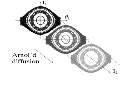
FIG. 1.: Three sections ($I_{1},\theta_{1}$) of the phase space for different values of $I_{2}$ are shown for the Hamiltonian (4) with the force (2) with $\mu=2\cdot 10^{-4}$, $f_{0}=2\cdot 10^{-6}$. The Arnol’d diffusion takes place along the $I_{2}$-direction, see details in the text.

We performed numerical study of the classical Arnol’d diffusion in the system described by the Hamiltonian (4). The frequencies of the perturbation (2) were chosen as $\Omega_{1}=0.2094$ and $\Omega_{2}=0.2513$ resulting in the period $T=150$. Therefore, $\omega=(\Omega_{1}+\Omega_{2})/2=0.23035$ which determines the amplitude $a\approx 0.2719$. Correspondingly, the initial conditions were taken for the system to be in between the two driving resonances.

To put the system inside the stochastic layer of the coupling resonance it is necessary to take $\theta_{1}=\pm\pi$. As in Ref.[10], the ratio $f_{0}/\mu=0.01$ was taken small enough in order to avoid the overlapping of three first-order resonances (see Eq.(13)). This also suppresses the influence of second-order resonances between unperturbed non-linear motion and the external perturbation.

Schematic structure of the coupling resonance is shown in Fig.1. Numerical data are obtained for different initial conditions corresponding to the separatrix layer and to the resonance region of the coupling resonance. The chaotic region inside the resonance is due to second-order resonances between non-linear motion of the unperturbed Hamiltonian and two-frequency perturbation. The condition of secondary resonances is $n\cdot\tilde{\omega}^{\prime}=m\cdot\delta\Omega$. Here $\tilde{\omega}^{\prime}$ is the frequency of oscillations at the coupling resonance (near the resonance centre we have $\tilde{\omega}^{\prime}\to\tilde{\omega}=\beta\sqrt{\mu}$), and $n,m$ are integers. One can find that the stochastic region inside the resonance corresponds to $m=1$ and $n=4$. As one can see, weak diffusion along the coupling resonance can occur both within the separatrix layer and inside the chaotic region formed by second-order resonances.

The diffusion coefficient was computed as follows,

$${\rm D}_{n}=\overline{(\Delta\bar{H})^{2}\over 10^{n}\cdot T}\,.$$ (16)

Here $\bar{H}$ is the value of the total Hamiltonian (4), averaged over time intervals $T_{n}$ of length $10^{n}\cdot T$ with $n=2,3$. The second average in (16) has been done in the following way. Having the mean value $\bar{H}$ in each interval $T_{n}$ for a fixed $n$, we computed the difference $\Delta\bar{H}$ between adjacent intervals, and averaged the variance $(\Delta\bar{H})^{2}$ over all differences. This procedure was taken in order to suppress large fluctuations of the energy, and to reveal a stochastic character of motion. Specifically, in the case of a true diffusion, one should expect $\rm D_{2}\approx\rm D_{3}$.

FIG. 2.: Dependence of the diffusion coefficient on initial conditions inside the coupling resonance, see details in the text.

The dependence of diffusion coefficients $D_{2}$ and $D_{3}$ on initial phase $\theta_{1}$ for $I_{1}=\theta_{2}=0$ and $I_{2}=\omega^{3}/(3\beta^{4})$ at $t=0$ is shown in Fig.2. The region close to $\theta_{1}=-\pi$ corresponds to initial conditions inside the separatrix layer, and the interval near $\theta_{1}=-\pi/2$ corresponds to initial conditions inside the inner stochastic region (see Fig.1). In both these regions Arnol’d diffusion coefficients have the same order. Approximate equality $\rm D_{2}\approx\rm D_{3}$ indicates here that the motion is really diffusion-like [10]. On the other hand, strong difference between ${\rm D}_{2}$ and ${\rm D}_{3}$ in the region $|\theta_{1}|<\pi/4$ manifests that the dynamics of the system is non-diffusive.

III Quantum model

The corresponding quantum model is described by the Hamiltonian (compare with Eq.(1)),

$$\hat{H}=\hat{H}^{0}_{x}+\hat{H}^{0}_{y}-\mu xy-f_{0}x(\cos\Omega_{1}t+\cos\Omega_{2}t).$$ (17)

Here

$$\hat{H}^{0}_{x}=\frac{\hat{p}_{x}^{2}}{2}+\frac{x^{4}}{4},\qquad\hat{H}^{0}_{y}=\frac{\hat{p}_{y}^{2}}{2}+\frac{y^{4}}{4},$$ (18)

and standard relations for momentum and coordinate operators are assumed,

$$[\hat{p}_{x},\,x]=-i\hbar_{0},\qquad[\hat{p}_{y},\,y]=-i\hbar_{0}$$ (19)

with the dimensionless Plank constant $\hbar_{0}$.

In order to investigate the evolution of the system, first, we have to find stationary eigenstates of the unperturbed ($f_{0}=0$) system, corresponding to the vicinity of the coupling resonance $\omega_{x}=\omega_{y}$. At the second stage, we will use the Floquet formalism when considering the time-periodic perturbation for $f_{0}\neq 0$. Specifically, we construct the evolution operator in one period $T$ of the perturbation, that allows one to study the dynamics over many periods.

A Stationary states of the coupling resonance

It is naturally to represent stationary states of the unperturbed Hamiltonian $\hat{H}_{s}$,

$$\hat{H}_{s}=\hat{H}^{0}_{x}+\hat{H}^{0}_{y}-\mu xy$$ (20)

in terms of the eigenstates of uncoupled ($\mu=0$) nonlinear oscillators,

$$\psi(x,\,y)=\sum_{n,m}c_{n,m}\psi^{0}_{n}(x)\psi^{0}_{m}(y).$$ (21)

Here $\psi^{0}_{n}(x)$, $\psi^{0}_{m}(y)$ are the eigenfunctions of $\hat{H}^{0}_{x}$, $\hat{H}^{0}_{y}$ (which will be calculated numerically), and the coefficients $c_{n,m}$ satisfy to the following stationary Schrödinger equation,

$$Ec_{n,m}=(E_{n}+E_{m})c_{n,m}-\mu\sum_{n^{\prime},m^{\prime}}x_{n,n^{\prime}}y_{m,m^{\prime}}c_{n^{\prime},m^{\prime}},$$ (22)

with $E_{n}$ and $E_{m}$ as eigenvalues of the Hamiltonians $\hat{H}^{0}_{x}$ and $\hat{H}^{0}_{y}$, respectively.

At the center of the coupling resonance $\omega_{n_{0}}=\omega_{m_{0}}$ we have $n_{0}=m_{0}$ and $\hbar_{0}\omega_{n_{0}}=E_{n_{0}}^{\prime}$, $\hbar_{0}\omega_{m_{0}}=E_{m_{0}}^{\prime}$. Near to this resonance it is convenient to expand $E_{n}$ and $E_{m}$ in Tailor series up to second order terms. This allows one to introduce new indexes $p=k+l$ and $k$ via the relations $n-n_{0}=k$ and $m-m_{0}=l$. Then our system (22) can be written in the following form,

$$\matrix{Ec_{k,p}=\left[\hbar_{0}\omega p+E_{n_{0}}^{\prime\prime}\left(k^{2}-pk+{p^{2}\over 2}\right)\right]c_{k,p}-\cr-\mu\Bigl{(}\dots+\sum_{k^{\prime}}x_{k,k^{\prime}}y_{p-k,-1-k^{\prime}}\,c_{k^{\prime},-1}+\Bigr{.}\cr\quad\;\;\,+\sum_{k^{\prime}}x_{k,k^{\prime}}y_{p-k,-k^{\prime}}\,c_{k^{\prime},0}+\cr\Bigl{.}\qquad\qquad\;\>\,+\sum_{k^{\prime}}x_{k,k^{\prime}}y_{p-k,1-k^{\prime}}\,c_{k^{\prime},1}+\dots\Bigr{)}}$$ (23)

with $\omega\equiv\omega_{n_{0}}$. One should note that matrix elements $x_{m,n}$ and $y_{m,n}$ of the coordinates $x$ and $y$ are equal to zero for transitions between the states of equal parity. Therefore, the exact solution of the system (23) is characterized by two independent sets of odd and even parity eigenstates (for odd and even $p$ respectively).

FIG. 3.: Energy spectrum of the system (23) in normalized units $e_{q,s}=E_{q,s}/\hbar_{0}\omega$ for $\mu=10^{-4}$, $\hbar_{0}=1.77321\cdot 10^{-5}$ and $n_{0}=446$. Three groups with 121 states in each group are shown.

Below we consider the case of a small nonlinearity,

$$\hbar_{0}\omega p\gg E_{n_{0}}^{\prime\prime}\left(k^{2}-kp+{p^{2}\over 2}\right).$$ (24)

This allows us to characterize all states by the group number $q$ and by the index $s$ that stands for energy levels inside each group. In fact, $q$ and $s$ are similar to fast and slow classical variables characterizing the motion inside the coupling resonance. Therefore, the energy in each group can be written as $E_{q,s}=\hbar_{0}\omega q+E^{M}_{q,s}$, where $E^{M}_{q,s}$ is the Mathieu-like spectrum of one group.

Numerical data for a fragment of the energy spectrum are shown in Fig.3. One can see that the spectrum consists of series of energy levels, shifted one from another by the value $\hbar_{0}\omega$. Note that the structure of the energy spectrum in each group is typical for a quantum nonlinear resonance [17]. Lowest levels are practically equidistant with the spacing equal to $\hbar_{0}\tilde{\omega}$, where $\tilde{\omega}$ is the classical frequency of small phase oscillations at the coupling resonance. Accumulation points correspond to classical separatricies, and all energy levels inside separatricies are non-degenerate. The states slightly above separatricies are quasi-degenerate due to the symmetry of a rotation in opposite directions.

FIG. 4.: Probability $|c_{k,p}|^{2}$ for eigenstates at the coupling resonance for $q=0$, $\mu=10^{-4}$ and different values of $s$. a) the lowest level (ground state) for $s=0$ ; b) near-separatrix level, $s=30$; c), d) above-separatrix levels, $s=\pm 35$.

Typical structure of eigenstates for different $s$ is shown in Fig.4. Note that ground states in each group correspond to $s=0$, and next stationary states, reordered according to the energy increase, are labelled by $1,-1,2,-2,\dots$ etc. The eigenstates inside the resonance are symmetrical with respect to $k=0$. One can see that the main maximum corresponds to $p=0$, although there are small additional maximums at $p=\pm 2,\pm 4,\dots$. The degree of delocalization in the $k$-space for eigenstates inside the coupling resonance strongly depends on the energy of eigenstates. Specifically, the closer the energy to that corresponding to the separatrix, the more delocalized is the eigenstate. Above the separatrix all eigenstates are characterized by the maximums of probability located symmetrically with respect to $k=0$ for states $s$ and $-s$, see Fig.4(c),(d).

B Evolution matrix

Now we consider the dynamics of our model in the presence of the external two-frequence perturbation acting on the $x$-oscillator. The frequencies $\Omega_{1}$ and $\Omega_{2}$ are commensurable, so that the external force is periodic with the period $T=iT_{1}=jT_{2}$, where $T_{1}=2\pi/\Omega_{1}$, $T_{2}=2\pi/\Omega_{2}$ and $i$, $j$ are integer. The initial conditions were taken for the system to be about half-way between the two driving resonances, $\omega=(\Omega_{1}+\Omega_{2})/2$.

Since the Hamiltonian (17) is periodic in time, in accordance with the Floquet theory the solution of the non-stationary Schrödinger equation can be written in the following form,

$$\psi(x,y,t)=\exp\left(-{i\varepsilon_{Q}t\over\hbar_{0}}\right)u_{Q}(x,y,t).$$ (25)

Here $u_{Q}(x,y,t)=u_{Q}(x,y,t+T)$ is the quasienergy function with the corresponding quasienergy (QE) $\varepsilon_{Q}$. The QE functions and quasienergies are, in fact, the eigenfunctions and eigenvalues of the evolution operator $\hat{U}(T)$ that describes the evolution of the system within one period of the external perturbation,

$$\hat{U}(T)u_{Q}(x,y)=\exp\left(-{i\varepsilon_{Q}T\over\hbar_{0}}\right)u_{Q}(x,y).$$ (26)

Since we are interested in wave functions only in discrete times $N\cdot T$ with $N$ integer, we omitted the argument $t$ in Eq.(26).

In order to construct the evolution operator, we represent the QE functions as follows,

$$u_{Q}(x,y)=\sum_{q,s}A^{Q}_{q,s}\psi_{q,s}(x,y).$$ (27)

Here the functions $\psi_{q,s}(x,y)$ are eigenstates of the stationary Hamiltonian $\hat{H}_{s}$ (see Eq.(20)), and the coefficients $A^{Q}_{q,s}$ are the eigenvectors of the operator $\hat{U}$ in the representation of $\hat{H}_{s}$. These eigenvectors can be found by a direct diagonalization of the corresponding matrix $U_{q,s;q^{\prime},s^{\prime}}$.

To obtain the matrix $U_{q,s;q^{\prime},s^{\prime}}$ we have used the following procedure. Let the evolution operator $\hat{U}$ act on an initial state $C^{\left(q_{0},s_{0}\right)}_{q,s}(0)=\delta_{q,q_{0}}\delta_{s,s_{0}}$. Then the wave function $C^{(q_{0},s_{0})}_{q,s}(T)$ at time $T$ forms the column of the evolution operator matrix,

$$\matrix{U_{q,s;q^{\prime},s^{\prime}}(T)C^{(q_{0},s_{0})}_{q^{\prime},s^{\prime}}(0)=U_{q,s;q_{0},s_{0}}(T)=C^{(q_{0},s_{0})}_{q,s}(T).}$$ (28)

Repetition of this procedure for different initial states $C^{(q^{\prime},s^{\prime})}_{q,s}(0)=\delta_{q,q^{\prime}}\delta_{s,s^{\prime}}$ allows one to find the whole matrix $U_{q,s;q^{\prime},s^{\prime}}(T)$. As a result, the wave function $C^{(q_{0},s_{0})}_{q,s}(T)$ can be computed numerically by integration of the nonstationary Schrödinger equation in the presence of the time-dependent perturbation,

$$\matrix{i\hbar_{0}\dot{C}_{q,s}=\left(\hbar_{0}\omega q+E^{M}_{q,s}\right)C_{q,s}-\cr-f_{0}\sum_{q^{\prime},s^{\prime}}x_{q,s;q^{\prime},s^{\prime}}\left(\cos\Omega_{1}t+\cos\Omega_{2}t\right)C_{q^{\prime},s^{\prime}}}$$ (29)

By introducing the slow amplitude $b_{q,s}(t)$ via the transformation

$$C_{q,s}(t)=b_{q,s}(t)\exp\left[-i\left(q\omega+E^{M}_{q,s}/\hbar_{0}\right)t\right]$$ (30)

one can obtain,

$$\matrix{i\hbar_{0}\dot{b}_{q,s}=-f_{0}\cos\left({\delta\Omega\over 2}t\right)\times\cr\times\sum_{s^{\prime}}\left[x_{q,s;q+1,s^{\prime}}\,b_{q+1,s^{\prime}}\,e^{-i\bigl{(}E^{M}_{q+1,s^{\prime}}-E^{M}_{q,s}\bigr{)}t/\hbar_{0}}+\right.\cr\left.\qquad\;+\,x_{q,s;q-1,s^{\prime}}\,b_{q-1,s^{\prime}}\,e^{-i\bigl{(}E^{M}_{q-1,s^{\prime}}-E^{M}_{q,s}\bigr{)}t/\hbar_{0}}\right],}$$ (31)

where $\delta\Omega=\Omega_{1}-\Omega_{2}$. In the resonance approximation we keep in Eq.(31) only the most important slowly oscillating terms with $q^{\prime}=q\pm 1$.

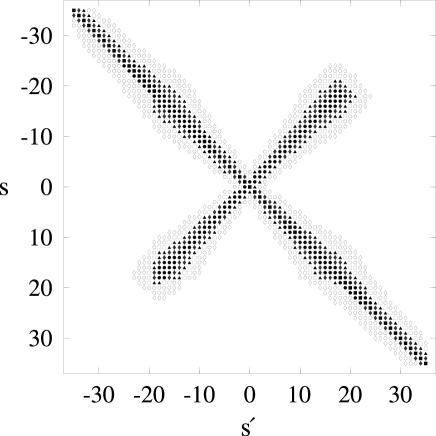
FIG. 5.: Matrix elements $|x_{q,s;q\pm 1,s^{\prime}}|$ that define the transition probability along the coupling resonance (for the same parameters as in Fig.3). Different values of the matrix elements are shown by grayscaled symbols. Black squares at the diagonal of the matrix have the values six orders of magnitude higher than those of matrix elements labeled by grey rhombuses.

The matrix elements $x_{q,s;q\pm 1,s^{\prime}}$ in Eq.(31) correspond to transitions between the states $s$ and $s^{\prime}$ from neighbor groups $q$ and $q\pm 1$. Figure 5 illustrates relative amplitudes of the matrix elements $|x_{0,s;1,s^{\prime}}|$. In accordance with our numeration of the states, matrix elements at the center of Fig.5 correspond to transitions between the lowest states in each group, and matrix elements at the corners define the transitions between the states above accumulation points. The latter elements quickly decrease with an increase of the difference $|s-s^{\prime}|$.

The “cross” at the center of Fig.5 where matrix elements are relatively large, corresponds to a transition between separatrix states. The important point is that the transition between such states of neighbor groups (along the coupling resonance) is much stronger than those between other states. This phenomenon is analogous to the quantum diffusion inside a separatrix, which was observed in [19] for a degenerate Hamiltonian system.

As a result, numerical procedure for computing the dynamics of our model is as follows. First, we solve Eqs.(31) and construct the evolution matrix $U_{q,s;q^{\prime},s^{\prime}}(T)$ by making use of Eq.(30). Then, direct diagonalization of this matrix yields the eigenvalues $\varepsilon_{Q}$ and the eigenvectors $A^{Q}_{q,s}$. Once the eigenvalues $\varepsilon_{Q}$ and eigenvectors $A^{Q}_{q,s}$ are obtained, one gets the evolution operator for one period,

$$U_{q,s;q^{\prime},s^{\prime}}(T)=\sum_{Q}A^{Q}_{q,s}{A^{Q^{\,*}}_{q^{\prime},s^{\prime}}}exp\left(-{i\varepsilon_{Q}T\over\hbar_{0}}\right).$$ (32)

By raising $U_{q,s;q^{\prime},s^{\prime}}(T)$ to the $N$-th power and using the ortogonality condition for the eigenvectors $A^{Q}_{q,s}$, one can obtain the evolution operator that propagates the system over $N$ periods of the external perturbation,

$$U_{q,s;q^{\prime},s^{\prime}}(NT)=\sum_{Q}A^{Q}_{q,s}{A^{Q^{\,*}}_{q^{\prime},s^{\prime}}}exp\left(-{i\varepsilon_{Q}NT\over\hbar_{0}}\right).$$ (33)

C Numerical data

As was shown above, in our model the Arnol’d diffusion occurs along the coupling resonance, or, the same, in $q$-space. This means that a wave packet initially localized at $q=0$, spreads diffusively in time. In order to observe this dynamics, below we introduce specific variables that characterize global structure of wave packets. But, first, we discuss the structure of QE eigenstates (in terms of these new variables) since it helps us to understand the mechanism of quantum Arnol’d diffusion.

In the $q$-space each of QE functions $A^{Q}_{q,s}$ can be globally characterized by the “mean position” $\bar{q}$ and by the variance $\sigma_{q}^{2}$ determined as follows [17, 18],

$$\bar{q}=\sum_{q}q\sum_{s}|A^{Q}_{q,s}|^{2},\,\,\,\,\,\,\,\,\,\sigma_{q}^{2}=\sum_{q}(q-\bar{q})^{2}\sum_{s}|A^{Q}_{q,s}|^{2}.$$ (34)

Then, it is convenient to plot $\bar{q}$ versus $\sigma_{q}$ for all eigenfunctions, see Fig.6. For small values of the coupling $\mu$, see Fig.6(a), the QE functions have a very small variance that means a strong localization in the $q$-space.

More details are seen in Fig.6(b) which shows a magnified fragment of Fig.6(a). One can see different groups of QE functions, characterizing specific relations between $\bar{q}$ and $\sigma_{q}$. First group consists of those eigenstates whose energies are close to the ground state (with a very small variance, $\sigma_{q}<10^{-3}$). Another group is characterized by an irregular dependence of $\bar{q}$ on $\sigma_{q}$ (region (1) in Fig.6(b)). The states which belong to this group are chaotic separtrix eigenstates. Regular dependences $\bar{q}(\sigma_{q})$ for $\sigma_{q}>10^{-3}$ correspond to under-separatrix states with $s>0$ and $s<0$. For very large $s$ this regular structure is destroyed due to the influence of two driving resonances (not shown in Fig.6(b)). Irregular spread of points in the region (2) reflects chaos in the inner region of the coupling resonance, that arises due to two secondary resonances $\hbar_{0}\delta\Omega/2=3E^{\prime\prime}_{n_{0}}(s+1/2)$. With an increase of $\mu$ (see Fig.6(c)), the regular structure of QE functions disappears. This means that many of eigenstates are chaotic. However, the variance $\sigma_{q}^{2}$ remains limited, thus, demonstrating that in the $q$ direction the eigenstates are localized. The fact that many points in Fig.6(c) are distributed incidentally, should be treated as the manifestation of quantum chaos.

FIG. 6.: Relation between $\bar{q}$ and $\sigma_{q}$ for the QE functions $A^{Q}_{q,s}$ in the region $q=0,\pm 1$ for different coupling constants: a,b) $\mu=3\cdot 10^{-5}$, c) $\mu=10^{-4}$. Each point corresponds to a specific QE function. Fig.6(b) shows the scaled-up fragment of the central part of Fig.6(a).

Now we discuss numerical results for the dynamics of our model. The evolution of any initial state $C_{q^{\prime},s^{\prime}}(0)$ can be computed using the evolution matrix $U_{q,s;q^{\prime},s^{\prime}}(NT)$,

$$C_{q,s}(NT)=\sum_{q^{\prime},s^{\prime}}U_{q,s;q^{\prime},s^{\prime}}(NT)C_{q^{\prime},s^{\prime}}(0).$$ (35)

We repeat again that our numerical data refer to the regime when the values of $\mu$ and $f_{0}$ are small enough, so that main three resonances are not overlapped.

Quantum dynamics for different initial conditions is shown in Fig.7. Here we show typical dependencies of the variance of the energy $\overline{(\Delta H)^{2}}=\hbar_{0}^{2}\omega^{2}\Delta_{q}$ in normalized units, versus time $t$ measured in the number $N$ of periods of the external perturbation. The quantity $\Delta_{q}$ is defined similar to that for the QE eigenstates, $\Delta_{q}=\sum_{q}(q-\bar{q})^{2}\sum_{s}|C_{q,s}|^{2}$ where $\bar{q}=\sum_{q}q\sum_{s}|C_{q,s}|^{2}$.

The data clearly show a different character of the evolution for three initial states taken from below and above the separatrix, as well as from the separatrix layer. For the states taken from the center of the resonance and well above the separatrix, the variance $\overline{(\Delta H)^{2}}$ quasi-periodically oscillates, in contrast with the separatrix state. In the latter case, after a short stochastization time the variance of the energy increases linearly in time, thus manifesting a diffusion-like spread of the wave packet.

FIG. 7.: Normalized variance $\Delta_{q}$ of the energy versus the rescaled time $N$ for 3 different initial states (for $\mu=1.25\cdot 10^{-4}$ and $f_{0}=1.25\cdot 10^{-6}$). Curves 1-3 correspond to an initial state near the center of the coupling resonance, above the separatrix, and from the separatrix layer, respectively.

More results are presented in Fig.8 where a diffusion-like increase of the energy is shown for separatrix initial states and different values of $\mu$. One can see that linear increase of the variance $\Delta_{q}(N)$ is typical, and it occurs after a short time which is associated with the time of a fast spread of packet over the separatrix layer in transverse direction. Such a behaviour is typical for the classical Arnol’d diffusion. The data allows one to determine the diffusion coefficient as $D={\overline{(\Delta H)^{2}}(N)}/(N\cdot T)$, by making use the fit to a linear dependence $\Delta_{q}(N)$ for $N>50$.

FIG. 8.: Time dependence of the variance of the energy for separatrix initial states and different values of coupling parameter $\mu$: 1) $\mu=10^{-4}$, 2) $\mu=1.25\cdot 10^{-4}$, 3) $\mu=1.75\cdot 10^{-4}$, 4) $\mu=2.25\cdot 10^{-4}$.

We have calculated separately quantum and classical diffusion coefficients and found that the quantum Arnol’d diffusion roughly corresponds to the classical one. However, the data clearly indicate that the quantum diffusion is systematically weaker than the classical Arnol’d diffusion, see Fig.9.

FIG. 9.: Quantum (squares) and classical (solid line) diffusion coefficients for different values of $\mu$.

One should stress that the quantum Arnol’d diffusion takes places only in the case when the number $M_{s}$ of energy stationary states in the separatrix layer is relatively large. For the first time, this point was noted by Shuryak [15] who studied the quantum-classical correspondence for nonlinear resonances. In this connection we have to estimate the number of the energy states that occupy the separatrix layer.

However, it is a problem to make reliable analytical estimates of the width of the separatrix layer for our model. As was shown in [20], in the case of many-frequency perturbation, secondary resonances play the dominant role in the formation of chaos in a separatrix layer. Indeed, as was shown above, the role of such resonances is quite strong in our case of the two-frequency perturbation. For this reason, we have performed a direct numerical calculation of the width of stochastic separatrix layer for the classical Hamiltonian, and used these results in order to estimate the number of separatrix energy levels in the corresponding energy interval.

We have found that for $\mu>1.25\cdot 10^{-4}$ the number $M_{s}$ of stationary states in the separatrix chaotic layer is more than 10, therefore, one can speak about a kind of stochastization in this region. On the other hand, with a decrease of the coupling (see data in Fig.9 for $1/\sqrt{\mu}>100$), the number $M_{s}$ decreases and for $\mu\approx 3\cdot 10^{-5}$ it is of the order one. For this reason the last right point in Fig.9 corresponds to the situation when classical chaotic motion along the coupling resonance is completely suppressed by quantum effects (the so-called “Shuryak border” [15]).

D Dynamical localization

Since the diffusive motion along the coupling resonance is effectively one-dimensional, one can naturally expect the Anderson-like localization. We have already noted that the variance of QE eigenstates of the evolution operator is finite in the $q$-space. This means that eigenstates are localized, and the wave packet dynamics in this direction has to reveal the saturation of the diffusion. More specifically, we expect that the linear increase of the variance of the energy ceases, after some characteristic time.

This effect known as the dynamical localization, has been discovered in [21, 22] for the kicked rotor, and was studied later in different physical models (see, for example, [1] and references therein). One should note that the dynamical localization is, in principle, different from the Anderson localization, since the latter occurs for models with random potentials. In contrast, the dynamical localization happens in dynamical (without any randomness) systems, and is due to interplay between (week) classical diffusion and (strong) quantum effects.

In order to observe the dynamical localization in our model (along the coupling resonance inside the separatrix layer), one needs to study long-time dynamics of wave packets. Our numerical study for large times $N\approx 10^{4}$ have revealed that after some time $t\sim t_{0}\approx 10^{3}\cdot T$, the diffusionlike evolution stops for all range of coupling parameter $\mu$. Instead, for larger times, the variance $\Delta_{q}$ starts to oscillate around the mean value $\overline{\Delta_{q}}$. Period of such oscillations depends on $\mu$ non-monotonically and vary from $10^{3}\cdot T$ to $10^{4}\cdot T$. Two examples of such a long-time dynamics are given in Fig.10.

FIG. 10.: Dynamical localization of wave packets inside the separatrix layer of the coupling resonance. The normalized variance of the energy is shown for different values of the coupling parameter: (1) $\mu=1.5\cdot 10^{-4}$, (2) $\mu=2.25\cdot 10^{-4}$. Horizontal dashed lines indicate the mean value $\overline{\Delta_{q}}$.

One can argue that the localization length is of the order of the width of wave packet after the saturation of the diffusion [22, 22]. Therefore, the localization length $l_{s}$ can be associated with the square root of $\overline{\Delta_{q}}$. We have numerically found the exponential dependence $\overline{\Delta_{q}}$ on $1/\sqrt{\mu}$, see Fig.11. This result is not surprising because $\log{D}$ is proportional to $1/\sqrt{\mu}$ (see Fig.9) and $t_{0}$ is practically independent on $\mu$.

FIG. 11.: The dependence of $\overline{\Delta_{q}}$ on $1/\sqrt{\mu}$.

It should be noted that the spread of packets in $k$ and $l$ space occurs even without the coupling between two resonances, due to the influence of the time-dependent perturbation (see Section III-A). For this reason one should compare this spread to that determined by the Arnol’d diffusion. Our additional study clearly show that these two effects are very different, see Fig.12.

FIG. 12.: Distribution of the probability $W_{q}$, averaged over time $t=10^{4}\cdot T$, versus the group number $q$: (1) $\mu=0$, $f_{0}=10^{-6}$; (2) $\mu=0$, $f_{0}=2\cdot 10^{-6}$; (3) $\mu=10^{-4}$, $f_{0}=10^{-6}$; (4) $\mu=2\cdot 10^{-4}$, $f_{0}=2\cdot 10^{-6}$.

Here, we plotted the profile $W_{q}=\sum_{s}|C_{q,s}|^{2}$ of the wave packet after the saturation, versus the group number $q$. This figure demonstrates the main effect of the Arnol’d diffusion along the coupling resonance. One can see that in all cases there is an exponential localization of packets in the $q$-space. This allows to introduce the localization length defined from the decrease of the probability in the tails of packets. The data illustrate a strong increase of the localization length in the presence of the coupling between two oscillators, in comparison with the case of completely independent oscillators for $\mu=0$ ($q=k+l$ and $l=0$).

IV Summary

We have studied the Hamiltonian system of two coupled nonlinear oscillators, one of which is under the influence of the time-dependent perturbation with two commensurate frequencies. In the classical description, the separatrix of the coupling resonance is destroyed due to the perturbation, and the Arnol’d diffusion occurs along this resonance inside a narrow stochastic layer. Our numerical data performed for the quantum analog of the system, allow us to make the following conclusions about the properties of the quantum Arnol’d diffusion.

By studying the quasienergy eigenstates of the evolution operator, we have found an irregular structure of those eigenstates which correspond to the stochastic layer. These eigenstates turned out to be exponentially localized along the coupling resonance, with the localization length, strongly enhanced in comparison with the case of non-coupled oscillators.

The study of wave packet dynamics for different initial states have revealed a diffusion-like spread of packets along the coupling resonance, if initial states correspond to the stochastic layer. We have found that the dependence of the diffusion coefficient on model parameters, roughly follows the classical dependence. However, the quantum diffusion is systematically slower than the classical one. This fact is obviously due to the influence of quantum effects.

It should be stressed that the quantum Arnol’d diffusion occurs in a deep semiclassical region, specifically, for the case when the number $M_{s}$ of chaotic eigenstates inside the stohastic layer is sufficiently large (of the order of 10 or larger). With a decrease of the coupling parameter, the diffusion coefficient strongly decreases, and for $M_{s}\leq 1$ the diffusion disappears. Therefore, we can see how strong quantum effects destroy the diffusive dynamics of wave packets.

Another manifestation of quantum effects is the dynamical localization that persists even for large $M_{s}$. Specifically, we have observed that the quantum diffusion occurs only for finite (although large) times. On a larger time scale the diffusion ceases, and after some characteristic time it terminates. This effect is similar to that discovered in the kicked rotor model [21] and studied later in other physical systems (see, for example, [1] and references therein). However, in our case the dynamical localization arises for a weak chaos inside the separatrix layer, in contrast to previous models with a strong (global) chaos in the classical description.

Our results may find a confirmation in experiments on one-electron dynamics in 2D semiconductor quantum billiards, where the charged particle motion is determined by the Hamiltonian of the type (17), (18). It is also possible that the quantum Arnol’d diffusion occurs in nuclear dynamics of complex molecules, driven by laser fields [23].

REFERENCES

- [1] A.J. Lichtenberg and M.A. Lieberman, Regular and Chaotic Dynamics, Springer-Verlag, New York (1992); L.E. Reichl, The Transition to Chaos, Springer-Verlag, New-York, 1992.
- [2] V.I. Arnol’d, DAN USSR, 156, 9 (1964) (in Russian).
- [3] Resonances in the Motion of Planets, Satellites and Asteroids, S. Ferraz-Mello and W. Sessin, eds. (Universidade de Sao Paulo, Sao Paulo, Brazil, 1985).
- [4] J. Binney and S. Tremaine, Galactic Dynamics, Princeton University Press, Princeton, N. J., 1987.
- [5] B.V. Chirikov, Phys. Rep., 52, 263 (1979).
- [6] Nonlinear Dynamics Aspects of Particle Accelerators, Lecture Notes in Physics, Springer-Verlag, Berlin, 247, 1986.
- [7] J. von Milczewski, G.H.F. Diercksen, and T. Uzer, Phys. Rev. Lett. 76, 2890 (1996).
- [8] D.M. Leitner and P.G. Wolynes, Phys. Rev. Lett., 79, 55 (1997).
- [9] B.V. Chirikov, E. Keil, and A.M. Sessler, J. Stat. Phys., 3, 307 (1971).
- [10] G.V. Gadiyak, F.M. Izrailev and B.V. Chirikov, Proceedings of the 7th International Conference on Nonlinear Oscillations, Berlin, (Akademie-Verlag, Berlin, 1977), Vol. II-1, p. 315; Institute of Nuclear Physics, Preprint 74-79, Novosibirsk, 1974.
- [11] B.V. Chirikov, J. Ford and F. Vivaldi, Nonlinear Dynamics and the Beam-Beam Interaction, Eds. M. Month and J.C. Herrera, A.I.P. Conf. Proc., 57, 323 (1979); J.L. Tennyson, M.A. Lieberman and A.J. Lichtenberg, ibid, p.272.
- [12] B.V. Chirikov and V.V. Vecheslavov, J. Stat. Phys., 71, 243 (1993); JETP, 112, 1132 (1997).
- [13] T.M. Fromhold et. al., Phys. Rev. Lett., 87, 046803 (2001).
- [14] A.A. Chernikov, R.Z. Sagdeev, D.A. Usikov, M.Yu. Zakharov, and G.M. Zaslavsky, Nature, 326, 559 (1987).
- [15] E.V. Shuryak, JETP, 71, 2039 (1976) (in Russian).
- [16] V.Ya. Demikhovskii, F.M. Izrailev, and A.I. Malyshev, Phys. Rev. Lett., 88, 154101 (2002).
- [17] G.P. Berman, O.F. Vlasova, and F.M. Izrailev, Zh. Eksp. Teor. Fiz. 93, 470 (1987) (in Russian); [English translation: Sov. Phys. JETP, 66, 269 (1987)].
- [18] M.Toda, Phys. Lett. A 110, 235 (1085).
- [19] V.Ya. Demikhovskii, D.I. Kamenev and G.A. Luna-Acosta, Phys. Rev. E, 59, 294 (1999); V.Ya. Demikhovskii, D.I. Kamenev, Phys. Lett. A, 228, 391 (1997).
- [20] V.V. Vecheslavov, JETP, 109, 2208 (1996) (in Russian).
- [21] G. Casati, B.V. Chirikov, F.M. Izrailev and J. Ford, Lect. Notes in Phys. 93 334 (1979).
- [22] B.V. Chirikov, F.M. Izrailev and D.L. Shepelyansky, Soviet Scientific Reviews, vol. 2C 209 (1981).
- [23] D.S. Perry, G.A. Bethardy, and M.J. Davis, J. Go, Discuss. Faraday Soc., 102, 215 (1995).