Relational Description of the Measurement
Process in Quantum Field Theory

Abstract

We have recently introduced a realistic, covariant, interpretation for the reduction process in relativistic quantum mechanics. The basic problem for a covariant description is the dependence of the states on the frame within which collapse takes place. A suitable use of the causal structure of the devices involved in the measurement process allowed us to introduce a covariant notion for the collapse of quantum states. However, a fully consistent description in the relativistic domain requires the extension of the interpretation to quantum fields. The extension is far from straightforward. Besides the obvious difficulty of dealing with the infinite degrees of freedom of the field theory, one has to analyze the restrictions imposed by causality concerning the allowed operations in a measurement process. In this paper we address these issues. We shall show that, in the case of partial causally connected measurements, our description allows us to include a wider class of causal operations than the one resulting from the standard way for computing conditional probabilities. This alternative description could be experimentally tested. A verification of this proposal would give a stronger support to the realistic interpretations of the states in quantum mechanics.

1 Introduction

In a previous paper, we have introduced a realistic, covariant, interpretation for the reduction process in relativistic quantum mechanics. The basic problem for a covariant description is the dependence of the states on the frame within which collapse takes place. More specifically, we have extended the tendency interpretation of standard quantum mechanics to the relativistic domain. Within this interpretation of standard quantum mechanics, a quantum state is a real entity that characterizes the disposition of the system, at a given value of the time, to produce certain events with certain probabilities. Due to the uniqueness of the non-relativistic time, once the measurement devices are specified, the set of alternatives among which the system chooses is determined without ambiguities. In fact, they are associated to the properties corresponding to a certain decomposition of the identity. The evolution of the state is also perfectly well defined. For instance, if we adopt the Heisenberg picture, the evolution is given by a sequence of states of disposition. The dispositions of the system change during the measurement processes according to the reduction postulate, and remain unchanged until the next measurement. Of course, the complete description is covariant under Galilean transformations.

In Ref[1] we proved that a relativistic quantum state may be considered as a multi-local relational object that characterizes the disposition of the system for producing certain events with certain probabilities among a given intrinsic set of alternatives. A covariant, intrinsic order was introduced by making use of the partial order of events induced by the causal structure of the theory. To do that, we have considered an experimental arrangement of measurement devices, each of them associated with the measurement of certain property over a space-like region at a given proper time. No special assumption was made about the state of motion of each device. Indeed, different proper times could emerge from this description due to the different local reference systems of each device. Thus, we may label each detector in an arbitrary system of coordinates by an open three-dimensional region $R_{a}$, and its four-velocity $u_{a}$. We now introduce a partial order in the following way: The instrument $A_{{R_{1}},{u_{1}}}$ precedes $A_{{R_{2}},{u_{2}}}$ if the region $R_{2}$ is contained in the forward light cone of $R_{1}$. Let us suppose that ${A^{0}}_{{R},{u}}$ precedes all the others. Then, it is possible to introduce a strict order without any reference to a Lorentz time as follows. Define $S^{1}$ as the set of instruments that are preceded only by $A^{0}$. Define $S^{2}$ as the set of instruments that are preceded only by the set $S^{1}$ and $A^{0}$. In general, define $S^{i}$ as the set of instruments that are preceded by the sets $S^{j}$ with $j<i$ and $A^{0}$. The crucial observation is that all the measurements on $S^{i}$ can be considered as ”simultaneous”. In fact, they are associated with local measurements performed by each device, and hence represented by a set of commuting operators. As the projectors commute and are self-adjoint on a “simultaneous” set $S^{i}$, all of them can be diagonalized on a single option. These conditions ensure that the quantum system has a well defined disposition with respect to the different alternatives of the set $S^{i}$. In other words one can unambiguously assign conditional probabilities after each measurement for the events associated to the set $S^{i}$.

In relativistic quantum mechanics, this description is only consistent up to lambda Compton corrections. In fact, the corresponding local projectors exist and commute, up to Compton wavelengths [1, 2, 3]. A fully consistent description of the measurement process in the relativistic domain requires the extension of the interpretation to quantum fields.This extension is far from trivial. Besides the obvious difficulty of dealing with the infinite degrees of freedom of the field theory, one has to face some issues related with the lack of a covariant notion of time order of the quantum measurements. In fact, there is not a well defined description for the Schroedinger evolution of the states on arbitrary foliations of space time, even for the free scalar quantum field in a Minkowski background.[4] Although the evolution is well defined in the Heisenberg picture, in general the operators associated with global space-time foliations are not self-adjoint. It is not guaranteed that in the particular case of the field operators this problem will appear. However, it is clear that a careful treatment is required in order to insure that they are well defined operators.

Another issue concerns the causal restrictions on the observable character of certain operators in Q.F.T. As it has been shown by many authors, causality imposes further restrictions on the allowed ideal operations on a measurement process. This observation arise when one considers some particular arrangements composed by partial causally connected measurements. It has been shown that while some operators are admissible in the relativistic domain, many others are not allowed by the standard formalism[5, 6, 9, 10]. Although this conclusion is correct, it is based on standard Bloch’s notion for ordering the events in the relativistic domain. Remember that Bloch’s approach consists on taking any Lorentzian reference system and hence:”…the right way to predict results obtained at $C$ is to use the time order that the three regions $A,B,C$ have in the Lorentz frame that one happens to be using”[11]. Nevertheless, we have introduced in [1] another covariant notion of partial order. Though both orders coincides in many cases, they imply different predictions for the cases of partial causally connected measurements. Here we shall show that our notion of intrinsic order allows us to extend the allowed causal operators to a wider and natural class.

In this paper we will consider the explicit case of a free, real, scalar field in a Minkowski space-time. The field operators smeared with local smooth functions are quantum observables associated with ideal measurement devices. They are associated to projectors corresponding to different values of the observed fields. We shall prove that the projectors associated with different regions of the $S^{i}$ option commute. This allows us to extend the real tendency interpretation to the quantum field theory domain giving a covariant description of the evolution of the states in the Heisenberg picture. As in relativistic quantum mechanics, the states are multi-local relational objects that characterize the disposition of the system for producing certain events with certain probabilities among a particular an intrinsic set of alternatives. The resulting picture of the multi-local and relational nature of quantum reality is even more intriguing than in the case of the relativistic particle. We shall show that it implies a modification of the standard expression for conditional probabilities in the case of partial causally connected measurements, allowing to include a wider range of causal operators. Our description could be experimentally tested. A verification of our predictions would give a stronger support to the realistic interpretations of the states in quantum mechanics.

The paper is organized as follows: In section 2, we develop our approach for a real free scalar field showing that it is possible to give a standard description of the measurement process of a quantum field. In section 3, we show that this approach is consistent with causality and provides predictions for conditional probabilities that differ from the standard predictions in the case of partial causally connected measurements. We also discuss the resulting relational interpretation of the quantum world. We present some concluding remarks in Section 4. The existence of the projectors as distributional operators acting on the Fock space is discussed in the Appendix.

2 The free K-G field

We shall study the relational tendency theory of a real free K-G field, evolving on a flat space-time. We start by considering the experimental arrangement of measurement devices, ${A^{f}}_{{R_{a}},{u_{a}}}$ each of them associated with the measurement of the average field

$${{\Phi}^{a}}\equiv{\Phi^{f^{a}}}_{R_{a}}(t^{L_{a}})=\int_{R_{a}}{f^{a}(y)\Phi(t^{L_{a}},y)d^{3}y}$$ (1)

where $f^{a}$ is a smooth smearing function with compact support such that it is non-zero in the $R_{a}$ region associated with the instrument that measures the field. The decomposition $(t^{L_{a}},x^{j})$ corresponds to the coordinates in the local Lorentz rest frame of the measurement device located in $R_{a}$.

The scalar field operators satisfy the field equations

$$({\eta}^{{\mu}{\nu}}{\nabla}_{\mu}{\nabla}_{\nu}-m^{2}){\Phi}=0$$ (2)

and the canonical commutation relations:

$$[{\Phi}(t^{L_{a}},y^{j}),{\Pi}(t^{L_{a}},x^{j})]=i{\delta}(x^{j}-y^{j})$$ (3)

$$[\Phi(t^{L_{a}},x^{j}),\Phi(t^{L_{a}},y^{j})]=0$$ (4)

Thus, we may write the field operator in terms of its Fourier components as follows:

$$\Phi(x^{\mu})={\int}d^{3}k[{\bf{a}}(k)g_{k}(x^{\mu})+{\bf{a}}^{\dagger}(k){g_{k}}^{\star}(x^{\mu})]$$ (5)

with

$$g_{k}=\frac{1}{\sqrt{{(2{\pi})^{3}}2{\omega}_{k}}}exp(-i{k^{\nu}}x_{\nu})$$ (6)

and

$$k_{0}={\omega}_{k}=+{\sqrt{{k^{j}}{k_{j}}+m^{2}}}$$ (7)

Generically, the devices belonging to the same set of alternatives $S^{i}$ will lie on several spatially separated non-simultaneous regions. Thus, in order to describe the whole set of alternatives in a single covariant Hilbert space ${\cal H}$ we will have to transform these operators to an arbitrary Lorentzian coordinate system. We shall exclude accelerated detectors, and consequently, we will have an unique decomposition of the fields in positive and negative frequency modes. This procedure allows us to define the Hilbert space in the Heisenberg picture on any global Lorentz coordinate system. The crucial observation is that all the measurements on $S^{i}$ can be considered as ”simultaneous”. In fact, two arbitrary devices of $S^{i}$ are separated by space-like intervals, and therefore, we shall prove that the corresponding operators ${\Phi^{a}}$, represented on ${\cal H}$, commute. What remains to be proved is that they are unbounded self-adjoint operators in the Fock space ${\cal F}$ of the scalar field and therefore they can be associated with ideal measurements. A measurement will produce events on the devices belonging to $S^{i}$ and the state of the field will collapse to the projected state associated to the set of outcomes of the measurement. The determination of the corresponding projectors is a crucial step of our construction. We are also going to prove that the construction is totally covariant and only depends on the quantum system, that is, the scalar field and the set of measurement devices. All the local operators $\Phi^{a}$ are represented on a generic Hilbert space via boosts transformations, and the physical predictions are independent on the particular space-like surface chosen for the definition of the inner product. Notice that we are not filling the whole space-time with devices. Instead we are considering a set of local measurements covering partial regions of space-time. If we had chosen the first point of view, we would run into troubles. Indeed, it was shown [4] that the functional evolution cannot be globally and unitarily implemented except for isometric foliations.

Once the projectors in the local reference frame of each detector has been defined, we need to transform them to a common, generic, Lorentz frame where all the projectors will be simultaneously defined. In other words, recalling that Hilbert spaces corresponding to two inertial systems of coordinates are unitarily equivalent we will represent all the projectors on the same space. The projectors and the smeared field operators transform in the same way, that is:

$${\Phi^{a}}_{L}=U^{-1}(L,L_{a}){{\Phi}^{a}}U(L,L_{a})$$ (8)

where $U(L,L_{a})$ is the unitary operator related to the boost connecting the generic Lorentz frame with the local frame of each device. Since we are dealing with the Heisenberg picture, the states do not evolve, and only the operators change with time. One can parameterize the evolution, with the time in the local reference frame of the device located in the region $R_{a}$, or what is equivalent with the proper time associated to this device. The projectors corresponding to the observation of a given value of the field ${\Phi}^{a}$ at a given proper time may be represented on the Hilbert space associated with any Lorentz frame.

We are now ready to study the spectral decomposition of the $\Phi^{a}$ operators. We start by solving the eigenvalue problem in the field representation. We shall work in the proper reference system where the measurement device is at rest. We shall proceed as follows, we start by choosing the field polarization and defining the Fock space. Then we shall determine the eigenvectors of the quantum observables $\Phi^{a}$, and show that they are well defined elements of the Fock space.

On this representation the field operators are diagonal and the canonical momenta are derivative operators,

$$<\phi|\Phi(x^{j})|\Psi>=\phi(x^{j})\Psi[{\phi}],$$ (9)

$$<\phi|\Pi(x^{j})|\Psi>=\frac{1}{i}\frac{\delta}{\delta\phi(x^{j})}\Psi[{\phi}].$$ (10)

The inner product is given by:

$$<\Psi(\phi)|\Gamma(\phi)>=\int D\phi{\Psi}^{*}(\phi)\Gamma(\phi)$$ (11)

and the eigenvectors of the field operators $|\phi>$ satisfy

$$<{\phi}|\tilde{\phi}>={\delta}(\phi-\tilde{\phi})$$ (12)

The fields transform as scalars under Lorentz transformations and the inner product is Lorentz invariant.

Let us now proceed to the construction of the Hamiltonian and the vacuum state in this representation.

The Hamiltonian operator is

$$H=\int_{\Sigma_{0}}{\frac{1}{2}[{\Pi^{2}}+\Phi{\hat{\omega}}^{2}\Phi}]$$ (13)

where

$${\hat{\omega}}^{2}={-{\nabla}}^{2}+m^{2}$$ (14)

The functional equation for the vacuum state, $\Psi_{0}[{\phi}]$, turns out to be:

$$\frac{1}{2}\left(\int_{\Sigma_{0}}{-\frac{{\delta}^{2}}{{\delta}\phi{\delta}\phi}}+\phi{\omega}^{2}{\phi}\right){\Psi_{0}}(\phi)=E_{0}{\Psi_{0}}(\phi).$$ (15)

The vacuum solution is of the form

$$\Psi_{0}[\phi]=det^{1/4}(\frac{\omega}{\pi})exp\left({-1\over 2}\int_{\Sigma_{0}}d^{3}zd^{3}x\phi(x^{j}){\omega}(z^{j}-x^{j})\phi(z^{j})\right)$$ (16)

where

$${\omega}(x^{j}-y^{j})=\sqrt{(-{{\nabla^{2}}_{x^{j}}}+m^{2})}\delta(x^{j}-y^{j})\equiv\int d^{j}kw_{k}e^{ik^{j}(x^{j}-y^{j})}$$ (17)

It can be easily seen that the energy of the ground state turns out to be $E_{0}=\frac{1}{2}tr{\omega}$ which diverges due to the zero mode contributions. The normalization factor also becomes infinite due to ultraviolet divergences. As it is well known and we shall show in what follows these infinities are harmless.

It is easy to show that the ground state is annihilated by:

$$a(x^{j})=\frac{1}{\sqrt{2}}\int_{\Sigma_{0}}d^{3}y{\omega}^{1/2}(x^{j}-y^{j})\Phi(y^{j})+i{\omega}^{-1/2}(x^{j}-y^{j})\Pi(y^{j}).$$ (18)

The Hamiltonian operator (13) is not well ordered, but its well ordered form may be immediately obtained by subtracting $E_{0}$. The corresponding creation operator may be immediately defined. The action of the Fourier component of the creation operator for the $k$ mode on the vaccuum state leads to the state $\Psi_{1}$ with eigenvalue $E_{1}=w_{k}+E_{0}$. The set of functional states given by the repeated action of the creation operator defines a basis of the Fock space. This is the orthonormal basis of ”functional Hermite polynomials” [7].

Now, we proceed to define the field operator in the proper Lorentz system. The Heisenberg equation for the field will read:

$$i{{\partial}\Phi\over{\partial}t}=[\Phi,H]$$ (19)

$$i{{\partial}\Pi\over{\partial}t}=[\Pi,H]$$ (20)

That is:

$$i{{\partial}\Phi\over{\partial}t}=\Pi$$ (21)

$$i{{\partial}\Pi\over{\partial}t}={\omega}^{2}\Phi$$ (22)

that leads to the K-G equation for the field operator. The general solution of this equation turns out to be:

$$\phi(x) = \int_{\Sigma_{0}}\phi(y)\stackrel{{\scriptstyle\leftrightarrow}}{{\partial_{n}}}D(x-y)dV$$ (23)

$$= \int_{\Sigma^{0}}\phi(y)\stackrel{{\scriptstyle\leftrightarrow}}{{\partial_{\mu}}}D(x-y)d\sigma_{\mu}$$

where $D$ is the homogeneous antisymmetric Klein-Gordon propagator. It can be easily seen, by making use of the Gauss Theorem, that this integral does not depend on the space-like surface. Thus, we can choose $\Sigma_{0}$ as the initial surface $y^{0}=0$ of the proper Lorentz system. It is easy to define, from this expression, the evolving operator. In fact, the solution depends on the value of $\phi$ and its temporal derivate, which is just its conjugate momentum $\Pi$, over $\Sigma_{0}$. Then the field will read:

$$\Phi(x^{j},t^{L_{a}})=\int_{\Sigma_{0}}dy^{3}\phi(y^{j}){\partial}_{y^{0}}D(x^{\mu},y^{j})-D(x^{\mu},y^{j}){1\over i}\frac{\delta}{\delta\phi(y^{j})}$$ (24)

We still have to show that the projectors corresponding to a measurement of the smeared field exist. More precisely, we will show that its action is well defined in the Hilbert space. We start with the determination of the eigenstates corresponding to the eigenvalue $\phi_{E}$ of the field operator $\Phi(x^{j},t^{L_{a}})$ on the proper system.

$$<\phi|\phi_{E},t^{L_{a}}>=Ce^{{i\over 2}<{\phi}A{\phi}>}e^{{i\over 2}<\phi_{E}A\phi_{E}>}e^{i<B{\phi_{E}}{\phi}>}$$ (25)

where $A$ and $B$ are propagators with Fourier components given by:

$$A(p,t^{L_{a}})\equiv\frac{\omega_{p}}{tan({\omega}_{p}t^{L_{a}})}$$ (26)

$$B(p,t^{L_{a}})\equiv\frac{\omega_{p}}{sin({\omega}_{p}t^{L_{a}})}$$ (27)

and we have used brackets for representing that the fields are integrated on $\Sigma_{0}$.

The normalization factor is determined by imposing the orthonormality of the eigenstates,

$$<\phi_{E},t^{L_{a}}|\phi_{E}^{\prime},t^{L_{a}}>=|C|^{2}e^{{-i\over 2}<{\phi}_{E}A{\phi}_{E}>}e^{{i\over 2}<{\phi}_{E}^{\prime}A{\phi}_{E}^{\prime}>}{\prod_{p}2\pi{sin({\omega}_{p}t^{L_{a}})\over{\omega}_{p}}}\delta(\phi_{E}(p)-\phi_{E^{\prime}}(p))$$ (28)

and it is given by:

$$C=\left(\prod_{p}{\frac{\omega_{p}}{{2\pi}isin(\omega_{p}t^{L_{a}})}}\right)^{1\over 2}$$ (29)

We also notice the interesting fact that if we take the limit:

$$<\phi|\phi_{E},t^{L_{a}}\rightarrow 0>=\left(\sqrt{\frac{1}{{2\pi}it^{L_{a}}}}\right)^{n}\exp{i\over 2}\left(\frac{(<\phi-\phi_{E}>)^{2}}{t^{L_{a}}}\right)$$ (30)

One recognizes the free propagator, and the delta function $\delta(\phi-\phi_{E})$ as one could expect.

One needs to introduce an infrared and ultraviolet regularization. The infrared regularization may be implemented by defining the fields in a periodic box. This allows to have a well defined normalization factor. The box will break the Lorentz invariance, but as we are dealing with local measurements, and we take the sides of the box much larger than the local region under study, this fact does not have any observable effect. We shall discuss the ultraviolet regularization later.

Let us now smear the field operators with smooth functions in order to have well defined eigenvectors. The smeared fields are the relational quantities that will be actually measured. Let us call $\phi_{\Delta}$ one of the eigenvalues that gives the real quantity $\Delta$ when smeared with the function $f^{a}$. That is, $\int_{R_{a}}f^{a}(y^{j})\phi_{\Delta}(y^{j})dy^{j}=\Delta$. Thus, $\Delta$ is the outcome of the relational observation. Let us denote the corresponding eigenstate $|\phi_{\Delta},t^{L_{a}}>$

Now we are ready for defining the projector for the $R_{a}$ region. It is given by:

$$<\phi|{P^{a}}_{F_{\Delta}}(t^{L_{a}})|\phi^{\prime}>=\int_{F_{\Delta}}d\Delta\int{d\phi_{\Delta}<\phi|\phi_{\Delta},t^{L_{a}}><\phi_{\Delta},t^{L_{a}}|\phi^{\prime}>\delta(<f^{a}\phi_{\Delta}>-\Delta)}$$ (31)

Where $F_{\Delta}$ is a partition of the possible values of $\Delta$. Notice that all the integrals are over the surface $\Sigma_{0}$ since $f^{a}$ has compact support in $R_{a}$.

Furthermore:

$$<\phi|{P^{a}}_{F_{\Delta}}(t^{L_{a}})|\phi^{\prime}>=$$

$$\int_{F_{\Delta}}d\Delta e^{{-i\over 2}<{\phi}A{\phi}>}e^{{i\over 2}<\phi^{\prime}A\phi^{\prime}>}\int d\alpha e^{-i\alpha\Delta}\prod_{p}\delta\left(\phi^{\prime}(p)-\phi(p)+\alpha\frac{sin(\omega_{p}t^{L_{a}})}{\omega_{p}}f^{a}(p)\right)$$ (32)

which is a functional distribution over the Hilbert space $L^{2}[d\phi]$, once the infrared regularization is taken into account.

For instance, if we compute its matrix elements among two vectors of the Hilbert space:

$$<\Psi(\phi)|{P^{a}}_{F_{\Delta}}(t^{L_{a}})|\Gamma(\phi)>=$$

$$\int_{F_{\Delta}}d\Delta\int d\alpha e^{-i\alpha\Delta}\int D\phi_{p}\Psi\left(\phi(p)+\alpha\frac{sin(\omega_{p}t^{L_{a}})}{\omega_{p}}f^{a}(p)\right)\Gamma(\phi(p))\times$$

$$e^{2i\alpha{\left(\frac{2\pi}{L}\right)^{3}}{\sum}_{p}f^{a}(p)cos(\omega_{p}t^{L_{a}})\phi(p)}e^{i\alpha^{2}{\left(\frac{2\pi}{L}\right)}^{3}{\sum}_{p}f^{a}(p)\frac{sin(\omega_{p}t^{L_{a}})cos(\omega_{p}t^{L_{a}})}{{\omega_{p}}}f^{a}(p)}$$ (33)

where $L^{3}$ is the volume of the box where we may put the field in order of avoiding the infrared divergences.

In order to prove that ${P^{a}}_{F_{\Delta}}(t^{L_{a}})$ is a projector we start by observing that:

$$\int{d\phi_{E}<\phi|\phi_{E},t^{L_{a}}><\phi_{E},t^{L_{a}}|\phi^{\prime}>}=\delta(\phi-\phi^{\prime})$$ (34)

This property allows us to construct a decomposition of the identity for a set of projectors associated to open portions $F_{\Delta}$ of the reals ${\cal R}$ such that $F_{\Delta}\cap F_{\Delta^{\prime}}=0$, and $\bigcup F_{\Delta}\sim{\cal R}$ up to a zero measure set. Therefore :

$$\sum_{F_{\Delta}}<\Psi(\phi)|{P^{a}}_{F_{\Delta}}|\Gamma(\phi)>=<\Psi(\phi)|\Gamma(\phi)>$$ (35)

Furthermore, if ${\tilde{\Delta}}\in F_{\Delta}$:

$${P^{a}}_{F_{\Delta}}(t^{L_{a}})|\phi_{\tilde{\Delta}},t^{L_{a}}>=|\phi_{\tilde{\Delta}},t^{L_{a}}>$$ (36)

If not:

$${P^{a}}_{F_{\Delta}}(t^{L_{a}})|\phi_{\tilde{\Delta}},t^{L_{a}}>=0$$ (37)

Finally two projectors associated to different spatial regions commute. This is a consequence of the commutation of the local operators $\Phi^{a}$. Indeed, if the local regions, $R_{a}$, $R_{b}$ define the same proper Lorentz frame the commutation of $\Phi^{a}$ and $\Phi^{b}$ for space-like separation is straightforward and hence the projectors commute. If the regions are not simultaneous, one needs to transform both operators to a common Lorentz frame. Let us call $U_{ab}$, the Lorentz transformation connecting both regions, then the relevant commutator will be $[{U_{ab}}^{\dagger}\Phi^{b}U_{ab},\Phi^{a}]$. As an arbitrary Lorentz boost may be written as a product of infinitesimal transformations, $U_{ab}=Id+{\epsilon}^{{\mu}{\nu}}M_{{\mu}{\nu}}$ it is sufficient to consider:

$${U_{ab}}^{-1}\Phi^{b}U_{ab}=\Phi^{b}+{\epsilon}^{{\mu}{\nu}}[M_{{\mu}{\nu}},\Phi^{b}]$$ (38)

The commutator of $M_{{\mu}{\nu}}$ with $\Phi^{a}$ only involve canonical operators evaluated at points of the region $R_{a}$, their commutator with operators associated to a region $R_{b}$ separated by a space-like interval will commute.

Thus, also for non-simultaneous regions, space-like separated projectors commute. In the Appendix we prove that this projectors have a well defined action on the Fock space of the free Klein Gordon field.

Thus the projectors associated to different local measurement devices on a “simultaneous” set $S^{i}$ commute and are self-adjoint. These properties insure that they can be diagonalized on a single set of alternatives, and the quantum system has a well defined, dispositional, state with respect to the different alternatives of the set $S^{i}$. In the Heisenberg picture, the evolution is given by a sequence of states of disposition. The dispositions of the system change during the measurement processes according to the reduction postulate, and remain unchanged until the next measurement. As in the case of relativistic quantum mechanics, the system provides, in each measurement, a result in devices that may be located on arbitrary space-like surfaces. Notice that contrary to what happens with the standard Lorentz dependent description of the reduction process, here the conditional probabilities of further measurements are unique. It is in that sense that the dispositions of the state to produce further results have an objective character.

3 Causality vs. the Intrinsic Order

As we mentioned before, it has been recently observed by many authors [5, 6, 9, 10] that the standard time order of ideal measurements in a Hilbert space may imply causal violations if partially connected regions are taken into account. Here we shall show that although this analysis is correct, it is based on a different notion for the ordering of the events. If one defines the partial order as we did in Ref [1], one may extend the causal predictions of the theory, and the reduction process is covariant and consistent with causality for a wide and natural class of operators.

Let us suppose, following Sorkin [6], that the devices performing the observation are not completely contained in the light cones coming from the previous set. We are therefore, interested in the case where only a portion of certain instrument is contained inside the light cone of the previous set. We could generalize the previously introduced notion of order by saying that $B$ follows the instrument $A$ if at least a portion of $B$ lies inside the forward light cone coming from $A$. With this ordering, let us to consider a particular arrangement for a set of instruments which measure a particular observable on a relativistic quantum system. Suppose three local regions: $A$, $B$, $C$ with their corresponding Heisenberg projectors: ${P^{A}}_{a}$, ${P^{B}}_{b}$, ${P^{B}}_{c}$ associated to values of certain Heisenberg observables over each region. We arrange the regions such that some points of $B$ follows $A$ and some points of $C$ follows $B$ but $A$ and $C$ are spatially separated(see figure 1)[6]. It is easy to build such arrangement, even with local regions. In this context, due to microcausality, the commutation relations between the observables and the projectors will be:

$$[{P^{A}}_{a},{P^{B}}_{b}]\neq 0$$ (39)

$$[{P^{B}}_{b},{P^{C}}_{c}]\neq 0$$ (40)

$$[{P^{A}}_{a},{P^{C}}_{c}]=0$$ (41)

Let us suppose that one uses this new notion of order, to define the sequence of options $S^{1}$,$S^{2}$, $S^{3}$ and the corresponding reduction processes followed by a quantum system. Then, since the new order implies $A<B<C$, one immediately notices that the $A$ measurement affects the $B$ measurement and also the $B$ measurement affects the $C$ measurements. Consequently, one should expect that the $A$ measurement would affect the $C$ measurement, leading to information traveling faster than light between $A$ and $C$, which are space-like separated regions.

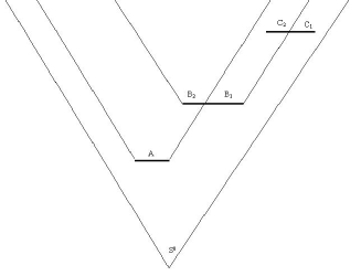
Figure 1: Sorkin’s arrangement with partial causally connected local regions.

One could immediately prove this fact as follows, let us suppose that the state of the field was prepared by a initial measurement, that precedes the whole arrangement, whose density operator we denote by $\rho_{0}$. Now, the probability of having the result $a,b,c$ in the regions $A,B,C$ given the initial state $\rho_{0}$ is, using Wigner’s formula:

$${\cal P}(a,b,c|\rho_{0})=Tr[{P^{C}}_{c}{P^{B}}_{b}{P^{A}}_{a}{\rho}_{0}{P^{A}}_{a}{P^{B}}_{b}]$$ (42)

This is the standard result that we would have obtained by making use of Bloch’s notion of order. Thus, one notices that an observer located in $C$ could know with certainty if a measurement has been performed by $A$. In fact, assume that a non-selective measurement has occurred on the region $A$, and ask for the probability of having $c$ under this hypothesis.

Then, one arrive to the probability:

$${\cal P}(\mathrm{unknown}\,a,b,c|\rho_{0})={{\sum}_{a}}\mathrm{Tr}[{P^{C}}_{c}{P^{B}}_{b}{P^{A}}_{a}{\rho}_{0}{P^{A}}_{a}{P^{B}}_{b}]$$ (43)

One immediately notices that this probability depends on whether the $A$ measurement was carried out or not, independently of the result. This is due the non-commutativity of the projector $P_{A}$ with $P_{B}$, and $P_{B}$ with $P_{C}$, that prevents us for using the identity ${\sum}_{a}{P^{A}}_{a}=Id$.

Notice that we have assumed that the $B$ measurement is known. However, since the $B$ region is partially connected with region $C$, a portion of $B$ will not be causally connected with $C$ and therefore, the preservation of causality would require that the measurement carried out by $B$ should be taken as non-selective respect to an observer localized on $C$.

If we take this fact into account one can prove that even with a non-selective measurement on $B$ one arrive to causal problems. In fact, we notice that the probability of having $c$, no matter

the result on $A,B$ is:

$${\cal P}(\mathrm{unknown}\;a,\mathrm{unknown}\;b,c|\rho_{0})=\sum_{a}\sum_{b}{\mathrm{Tr}}[{P^{C}}_{c}{P^{B}}_{b}{P^{A}}_{a}{\rho}_{0}{P^{A}}_{a}{P^{B}}_{b}],$$ (44)

which depends on whether or not the $A$ and $B$ measurements were carried out. Hence, if one starts from a different definition of the partial ordering of the alternatives, in terms of a partial causal connection, one gets faster than light signals for a wide class of operators which prevent us to eliminate the $A$ measurement. In those cases the observer $C$ could know with certainty if the previous two measurements were carried out or not. There is not any violation with respect to the $B$ observation since an observer at $C$ may be causally informed about a measurement carried out at $B$. However, the above analysis implies faster than light communication with respect to the $A$ measurement since it is space-like separated from $C$. Therefore, the requirement of causality strongly restricts the allowed observable quantities in relativistic quantum mechanics.

In what follows we are going to show that our description is consistent with causality for a wider range of operations. The key observation is that our notion of partial ordering requires to consider the instruments as composed of several parts each one associated to different measurement processes. That is, in the case where only a portion of the instrument is causally connected, one needs to decompose the devices in parts such that each part is completely inside (or outside) the forward light cone coming from the previous devices. Now the alternatives belonging to one option $S^{i}$ are composed by several parts of different instruments. In fact, a particular device could contain parts belonging to different options. Although the measurement performed by any device is seen as Lorentz simultaneous for any local reference system it will be associated to several events.

Let us reconsider the previous example with our notion of order (see figure 1). Let us start with $S^{0}$ and the preparation of the state in $\rho_{0}$. We will call ($B_{1}$) the part of $B$ non-casually connected with $A$ and ($C_{1}$) the part of $C$ non causally connected with $B$. The part of $B$ causally connected with $A$ ($B_{2}$) and the part of $C$ causally connected with $B$ ($C_{2}$). Now we can construct the set of options as, $S^{1}=(A,B_{1},C_{1})$ then $S^{2}=(B_{2},C_{2})$.

Thus, we need to deal with partial observations. Let us consider the case where the operator associated to the measurement carried out on $C$ may be taken as composed by two partial operators associated to $C_{1}$ and $C_{2}$, We shall denote the respective eigenvalues as $c_{1}$ and $c_{2}$. Notice that, the individuality of the device still persists since we do not have access to each result but only to the total result $c$ obtained on $C$ after the observation. Now it is important to consider how one gets $c$ through $c_{1}$ and $c_{2}$. Let us assume that the result $c$ is extensive in the sense that $c=f(c_{1},c_{2})$. This relation depends on the particular observation we are performing on each alternative. For instance, let us call $(O^{1},O^{2})$ the local operators associated to the observations on $(C_{1},C_{2})$ and $O$ the operator associated to $C$. Therefore, $f(O^{1},O^{2})=O$ is the functional relation between them. For the case of the field measurements, we will have $f\equiv c_{1}+c_{2}$ which is just the relation $\Phi^{C_{1}}+\Phi^{C_{2}}=\Phi^{C}$. Notice however, that this hypothesis also includes a wide range of observables. Indeed, it allows us to measure local operators which involve products of multiple smeared fields. These operators will imply indeed a non linear behavior for the functional relation $f(c_{1},c_{2})=c$. Now we can compute the probability of observing $c$ for selective measurements in $A,B$ given the initial state $\rho_{0}$. In first place, we have to deal with the measurement of $b$ occurring on $B$. As we have divided the device in two portions, this result will be composed by two unknown measurements $b_{1}$ and $b_{2}$, such that $b=f(b_{1},b_{2})$. Analogously for the probability of having $c$ since it results from two independent measurements in $C_{1}$ and $C_{2}$. Thus, we will have:

$${\cal P}(a,b,c|\rho_{0})={\sum}_{(c_{1},c_{2},b_{1},b_{2})}\delta(c-f(c_{1},c_{2}))\delta(b-f(b_{1},b_{2}))\times$$ (45)

$$\times Tr[{P^{C_{2}}}_{c_{2}}{P^{B_{2}}}_{b_{2}}{P^{B_{1}}}_{b_{1}}{P^{C_{1}}}_{c_{1}}{P^{A}}_{a}{\rho}_{0}{P^{A}}_{a}{P^{C_{1}}}_{c_{1}}{P^{B_{1}}}_{b_{1}}{P^{B_{2}}}_{b_{2}}])=$$

$$\sum_{b_{1}}\sum_{b_{2}}\delta(b-f(b_{1},b_{2}))Tr[{P^{C}}_{c}{P^{B_{2}}}_{b_{2}}{P^{B_{1}}}_{b_{1}}{P^{A}}_{a}{\rho}_{0}{P^{A}}_{a}{P^{B_{1}}}_{b_{1}}{P^{B_{2}}}_{b_{2}}]$$

Where we have taken into account that, due to microcausality:

$${P^{C}}_{c}=\sum_{c_{1}}\sum_{c_{2}}\delta(c-f(c_{1},c_{2})){P^{C_{1}}}_{c_{1}}{P^{C_{2}}}_{c_{2}}$$ (46)

The sum on $b_{1},b_{2}$ goes over the complete set of possible results. The same applies for the $C$ measurement.
Now, in order to study the causal implications we need to compute the probability of having $c$ for non-selective measurements on $A,B$. Therefore, one gets:

$${\cal P}(\mathrm{unknown}\;a,\mathrm{unknown}\;b,c|\rho_{0})=\sum_{a}\sum_{b}{\cal P}(c,a,b|\rho_{0})=$$ (47)

$${\sum}_{(c_{1},c_{2},b_{1})}\delta(c-f(c_{1},c_{2}))Tr[{P^{C_{2}}}_{c_{2}}{P^{B_{1}}}_{b_{1}}{P^{C_{1}}}_{c_{1}}{\rho}_{0}{P^{C_{1}}}_{c_{1}}{P^{B_{1}}}_{b_{1}}]=\sum_{b_{1}}Tr[{P^{C}}_{c}{P^{B_{1}}}_{b_{1}}\rho_{0}{P^{B_{1}}}_{b_{1}}]$$

Where we have used that $\sum_{b_{2}}{P^{B_{2}}}_{b_{2}}=Id$. Thus, this probability does not depend on the $A$ measurement and our description does not lead to any violation of causality during the measurement process.

Although there is some kind of correlation introduced by the causally connected part of $B$ with $C$, we will not have any information about the actual observation made on $B$, as we noticed before. This correlation is very interesting and could be experimentally tested. Notice that only the assignment of probabilities given by equations (3,47) is consistent with causality for the general kind of measurements that we have considered.

Several issues concerning the relational interpretation can be read from the previous analysis. The devices never lose their individuality as instruments of measurement of a certain observable, for instance, the local field on certain region. However what is quite surprising is that while the devices are turned on for a local proper time $T$, the ”decision” made by the quantum system with respect to this region is taken by two non-simultaneous processes within the given intrinsic order. The local time of measurement is quite different to the internal order for which the ”decisions” were taken. Now, the set of ”simultaneous” alternatives is composed by portions of several devices. The individuality of each device is preserved, since we do not have access to the results of these partial alternatives. What we observe in each experiment is the total result registered by each device.
Another consequence of our approach concerns the causal connection among alternatives belonging to different sets $S^{j}$. As we have shown, there is correlation among the causally connected portions of different devices, nevertheless this correlation does not imply any incompatibility with causality.
All these features show a global aspect of the relational tendency interpretation which is very interesting since the decomposition is produced by the global configuration of the measurement devices evolving in a Minkowski space-time, without any reference to a particular Lorentz foliation.

We have considered a measurement arrangement which is reminiscent to the observation of a non-local property [5]. We can indeed naturally extend our approach to the case of widely separated non-local measurements, or even widely extended observation. Now the partial causal connection is simply implemented taken Sorkin’s arrangement, on figure 1, modified to the case of measurements carried out on disconnected regions $B,C$, or even a space-like surface. The conclusion is the same. In the cases of partial causally connected measurements our description includes a wider range of causal operators than the standard approach.

4 Conclusions

We have developed the multi-local, covariant, relational description of the measurement process of a quantum free field. We have addressed the criticisms raised by various authors to the standard Hilbert approach and shown that they are naturally avoided by our covariant description of the measurement process. In order to address these issues, we have extended the intrinsic order associated to a sequence of measurements to the case of partially connected measurement devices. This extension has further implications on the relational meaning of the measurement process. A particular measurement process of a given property performed by a given measurement device on a region of space-time, should be considered as composed by a sequence of decision processes occurring on different regions of the device. This solves the causal problems and implies a global relational aspect of the complete set of alternatives $S^{i}$. From an observational point of view, we have proved that causality holds in the canonical approach for a wide and natural class of operators, while the standard formalism is extreemly restrictive. Our proposal could be experimentally tested trough the implementation of the particular configuration proposed in the previous section. Furthermore, our predictions for the reduction of the states should be associated to the decision process during the interaction of the quantum system with the measurement devices and may be considered, if confirmed, as an experimental evidence of the physical character of the quantum states. If this is experimentally verified, the standard instrumentalist approach introduced by I.Bloch concerning the measurement process in relativistic quantum mechanics, would not be compatible with experiments. This is mainly due to the fact that this order does not coincide with our intrinsic order in the case of partially connected regions, and Bloch’s approach would not be in general compatible with causality for the measurements we have considered.

It is now clear that the description that we have introduced has a relational nature. Firstly because the intrinsic order of the options $S^{i}$ is defined in relational terms by the measurement devices. But also because self-adjoint operators may only be defined if they are associated to a set of local devices. Recall that self-adjoint global operators that describe the field on arbitrary spatial hyper-surfaces do not exist.
The tendency interpretation of non-relativistic quantum mechanics is naturally a relational theory. If one thinks, for instance, in the solution proposed by Bohr for the EPR paradox [13] one immediately recognizes that one cannot associate a given reality to a quantum system before measurement. Even the Unruh effect for accelerated detectors has a very deep relational meaning. As Unruh noticed: ”A particle detector will react to states which have positive frequency respect to the detectors proper time, not with respect to any universal time[14].
One of the main challenges of the XXI century is the conclusion of the XX revolution toward a quantum theory of gravity. The relational point of view is crucial in both theories, the quantum and the relativistic. We have proposed a possible interpretation for any canonical theory in the realm of special relativity. How to extend it to gravity implies further study, mainly because of the nonexistence of a natural intrinsic order without any reference to a space-time background. Furthermore, up to now there is no evidence of local observables in pure quantum gravity. This is another evidence of the relational character of the theory. We are now studying these issues.

5 Acknowledgments

We would like to thank Michael Reisenberger for very useful discussions and suggestions about the presentation of this paper.

6 Appendix

Here, we prove that the projector is a well defined operator in the Fock space.

Let us start by looking at the quantity $<\phi_{\Delta},t^{L_{a}}|0>$:

$$<\phi_{\Delta},t^{L_{a}}|0>=Cdet^{1/4}(\frac{\omega}{\pi})e^{{-i\over 2}<{\phi}_{\Delta}A{\phi}_{\Delta}>}\int D\phi e^{{-1\over 2}<{\phi}(\omega+iA){\phi}>}e^{-i<B{\phi}_{\Delta}{\phi}>}$$ (48)

Hence:

$$<\phi_{\Delta},t^{L_{a}}|0>=C\frac{det^{1/4}(\frac{\omega}{\pi})}{det^{1/2}(\frac{(\omega+iA)}{2\pi})}e^{{-i\over 2}<{\phi}_{\Delta}A{\phi}_{\Delta}>}exp\left({-1\over 2}<{\phi}_{\Delta}B(\omega+iA)^{-1}B{\phi}_{\Delta}>\right)$$ (49)

This turns out to be:

$$<\phi_{\Delta},t^{L_{a}}|0>=\left(\prod_{p}e^{i\omega_{p}t^{L_{a}}\over 2}\right){det^{1/4}(\frac{\omega}{\pi})}e^{{-1\over 2}<\phi_{\Delta}\omega\phi_{\Delta}>},$$ (50)

which is just the vacuum state, evaluated for $\phi_{\Delta}$, up to a global phase. This result is a consequence of the Poincare invariance of the vacuum, modulo the zero mode, and of the fact that in the limit when $t^{L_{a}}$ tends to zero $|\phi_{\Delta},t^{L_{a}}>$ is just $|\phi_{\Delta}>$.

Furthermore, the mean value of the projector ${P^{a}}_{F_{\Delta}}(t^{L_{a}})$ in the vacuum state is given by:

$$<0|{P^{a}}_{F_{\Delta}}(t^{L_{a}})|0>=det^{1\over 2}\left({\omega\over\pi}\right)\int_{F_{\Delta}}d\Delta\int d\phi_{\Delta}\int d\alpha e^{-<\phi_{\Delta}\omega\phi_{\Delta}>}e^{i\alpha(<f^{a}\phi_{\Delta}>-\Delta)}$$ (51)

That is,

$$<0|{P^{a}}_{F_{\Delta}}(t^{L_{a}})|0>=\int_{F_{\Delta}}d\Delta\frac{2\pi}{\sqrt{<f^{a}{\omega}^{-1}f^{a}>}}exp\left(\frac{-{\Delta}^{2}}{4<f^{a}{\omega}^{-1}f^{a}>}\right)$$ (52)

which leads to:

$$<0|{P^{a}}_{F_{\Delta}}(t^{L_{a}})|0>=\int_{F_{\Delta}}d\Delta\frac{2\pi}{\sqrt{{\left(\ \frac{2\pi}{L}\right)^{3}}\sum_{p}{\frac{|f^{a}(p)|^{2}}{\omega_{p}}}}}exp\left(\frac{-{\Delta}^{2}}{{\left(\frac{2\pi}{L}\right)^{3}}{\sum}_{p}{\frac{|f^{a}(p)|^{2}}{\omega_{p}}}}\right)$$ (53)

where $L^{3}$ is the volume of the box where the fields live.

Several issues may be learned from this expression. First of all, as it should be, one gets a Gaussian distribution around the zero value. Furthermore it is divergent free, provided the integral $\int dp{\frac{|f^{a}(p)|^{2}}{\omega_{p}}}$ gives a finite result. This is achieved by demanding that the smearing functions do not contain high Fourier components.

In order to complete the proof we are going to show that the projector is well defined on the complete Fock space.

To begin with, we take the single particle state:

$$<{\phi}|1_{k}>=\sqrt{2\omega_{k}}\int_{\Sigma_{0}}d^{j}ye^{ik_{j}y^{j}}\phi(y^{j})\Psi_{0}[\phi]\equiv\sqrt{2\omega_{k}}\phi(k_{j})\Psi_{0}[\phi]$$ (54)

Now we calculate $<\phi_{\Delta},t^{L_{a}}|1_{k}>$ getting:

$$<\phi_{\Delta},t^{L_{a}}|1_{k}>=C{det^{1/4}(\frac{\omega}{\pi})}\sqrt{2\omega_{k}}e^{{-i\over 2}<{\phi}_{\Delta}A{\phi}_{\Delta}>}{\times}$$

$$\int D\phi(p_{j})\phi(k_{j})e^{{-1\over 2}{\left(\frac{2\pi}{L}\right)^{3}}\sum_{p}{\phi}(p_{j})({\omega}_{p}+iA(p,t^{L_{a}})){\phi}(p_{j})}e^{-i{\left(\frac{2\pi}{L}\right)^{3}}\sum_{p}B(p,t^{L_{a}}){\phi}_{\Delta}(p_{j}){\phi}(p_{j})}$$ (55)

As one immediately notices the main difference is the resulting multiplicative factor associated with a single mode $\phi(k_{j})$.

In order to include the general, many particle, case, one could introduce a source term $J$ and define a generating functional $Z(J)$ as follows:

$$Z(J)=<\phi_{\Delta},t^{L_{a}}|0>^{J}{\equiv}C{det^{1/4}(\frac{\omega}{\pi})}e^{{-i\over 2}<{\phi}_{\Delta}A{\phi}_{\Delta}>}\times$$

$$\int D\phi(p_{j})e^{{-1\over 2}{\left(\frac{2\pi}{L}\right)^{3}}\sum_{p}{\phi}(p_{j})({\omega}_{p}+iA(p,t^{L_{a}})){\phi}(p_{j})}e^{-i{\left(\frac{2\pi}{L}\right)^{3}}\sum_{p}\left(B(p,t^{L_{a}})\phi_{\Delta}(p_{j})+J(p_{j})\right){\phi}(p_{j})}$$ (56)

It is easy to show that indeed:

$$<\phi_{\Delta},t^{L_{a}}|1_{k}>=\sqrt{2\omega_{k}}\frac{i\delta}{\delta J(k)}Z(J){\mid}_{J=0}$$ (57)

This procedure may be identified with the usual one in Q.F.T., We will call, $n$-point function the $n$ functional derivative respect to $J(k^{1})...J(k^{n})$.
Now, it is not difficult to show that the inner product $<n_{1}....n_{k}...|\phi_{\Delta},t^{L_{a}}>$, may be calculated, up to multiplicative factors, in terms of the $n$-point functions. Those factors are functions of the frequencies of the modes involved in the given Fock state.
To do that, we start by studying the form of the particle states in Fock space. The Fock space is constructed by the creation operators. Their action applied to the vacuum in the field representation, consists in the multiplication by some $k$ dependent component of the field ($\phi(k)$) and a derivative of the vacuum state respect to this mode corresponding to the given particle state we were creating. Due the structure of the vacuum, this derivative term also leads to a multiplicative factor. It is indeed the mode $\phi_{k}$ multiplied by some function of the frequency of the particular mode. Furthermore it gives a finite result since the Fock space is made by finite set of particle states. Therefore, the Fock $n$-particle states in the functional representation, are obtained by multiplying the vacuum by a set of $k$-dependent components of the field multiplied by some functions of the frequencies of each mode in the state. This is exactly the form of the n-point functions obtained from the generating function $Z(J)$.

The only remaining issue is the computation of $Z(J)$. One can show that, after the functional integration is performed, one arrives to:

$$Z(J)=\left(\prod_{p}e^{i\omega_{p}t^{L_{a}}\over 2}\right){det^{1/4}(\frac{\omega}{\pi})}e^{{-1\over 2}<\phi_{\Delta}\omega\phi_{\Delta}>}e^{{-1\over 2}<J(\omega+iA)^{-1}J>}e^{-<J(\omega+iA)^{-1}B\phi_{\Delta}>}$$ (58)

The divergent multiplicative factor coming from the normalization of the vacuum disappears when we take the projector as in (52). Furthermore the matrix elements of the projector in the Fock space are given by:

$$<n_{1}..n_{k}..|{P^{a}}_{F_{\Delta}}|n^{\prime}_{1}..n^{\prime}_{k}..>=$$

$$\int_{F_{\Delta}}d\Delta\int d\alpha d\phi_{\Delta}<n_{1}..n_{k}..|\phi_{\Delta},t^{L_{a}}><\phi_{\Delta},t^{L_{a}}|n^{\prime}_{1}..n^{\prime}_{k}..>e^{i\alpha(<f^{a}\phi_{\Delta}>-\Delta)}$$ (59)

Since the inner product $<n_{1}....n_{k}...|\phi_{\Delta},t^{L_{a}}>$ is a sum of a set of $n$-point functions times some finite functions of the $k$-modes of the particular state under consideration, we can write them as derivatives of $Z(J)$ and take out of the integral the derivatives with respect to $J_{i}$. Hence in the integral part it remains a divergent factor $|{det^{1/2}(\frac{\omega}{\pi})}|\times e^{-<\phi_{\Delta}\omega\phi_{\Delta}>}$ coming from the vacuum state. However, the $d\phi_{\Delta}$ integral is quadratic in the field and contributes with a factor that cancels this infinite, as before. This is a well known fact, as it was noticed by Jackiw [7], the divergent factor $det^{1/4}(\frac{\omega}{\pi})=exp{V\over 4}\int d^{j}k{1\over\pi}ln\sqrt{k^{2}+m^{2}}$ , which is ultraviolet divergent, does not affect matrix elements between states on the Fock space since it is chosen in such a way that it it disappears from the final expression. Thus, the matrix elements of the projector are well defined in the Fock space and we arrive to a well defined quantum field theory as it was required.

References

- [1] R. Gambini and R. A. Porto, Phys. Lett. A Volume 294, Issue 3 (129-133), (2002).
- [2] R. Gambini and R. A. Porto, Phys. Rev. D 63, 105014, (2001)
- [3] D. Marolf and C. Rovelli, e-print gr-qc/0203056
- [4] Ch.Torre and M. Varadarajan, Class. Quant. Grav. 16, 2651, (1999)
-
[5]
Y.Aharonov and D.Albert, Phys. Rev. D.
21, 3316,(1980)
Y.Aharonov and D.Albert, Phys. Rev. D. 24, 359,(1981)
Y.Aharonov and D.Albert, Phys. Rev. D. 29, 228, (1984). - [6] R.Sorkin, ”Directions in General Relativity, vol. II: a collection of Essays in honor of Dieter Brill’s Sixtieth Birthday” (CUP, 1993) B.L. Hu and T.A. Jacobson eds.
- [7] R. Jackiw, ”Field theoretic results in the Schroedinger representation” Lecture presented at 17th Int. Colloq. on Group Theoretical Methods in Physics, St. Adele, Canada, (1988)
- [8] J.M. Mourao, T. Thiemann, and J.M. Velhinho, J. Math. Phys. 40 2337 (1999)
- [9] D. Beckman, D.Gottesman, M.A. Nielsen and J.Preskill Phys.Rev. A 64 (2001) 052309.
- [10] D. Beckman, D.Gottesman, A. Kitaev and J.Preskill Phys. Rev.D 65, 065022 (2002).
- [11] I.Bloch, Phys. Rev. 156, 1377, (1967)
- [12] A. Corichi, M.P. Ryan and D. Sudarsky, e-print gr-qc/0203072.
- [13] N. Bohr, Phys. Rev 48, 696, (1935)
- [14] W.G. Unruh, Phys Rev. D. 14, 870, (1976)