Creation of Entanglement by Interaction with a Common Heat Bath

Abstract

I show that entanglement between two qubits can be generated if the two qubits interact with a common heat bath in thermal equilibrium, but do not interact directly with each other. In most situations the entanglement is created for a very short time after the interaction with the heat bath is switched on, but depending on system, coupling, and heat bath, the entanglement may persist for arbitrarily long times. This mechanism sheds new light on the creation of entanglement. A particular example of two quantum dots in a closed cavity is discussed, where the heat bath is given by the blackbody radiation.

Since the discovery of quantum mechanics, “entanglement” has been considered a hallmark of quantum behavior [1]. Two quantum systems $A$ and $B$ in a pure state are called entangled, if their quantum mechanical state vector $|\psi\rangle$ can not be written as product of two states $|\phi_{A}\rangle$ and $|\phi_{B}\rangle$ in the Hilbert spaces of $A$ and $B$, respectively. The last few years of research on quantum information processing have lead to the picture of entanglement as a precious resource. Entanglement plays an important role in super–dense coding [2] and quantum teleportation [3], and is necessary for the exponential speed–up of quantum algorithms compared to classical algorithms [4].

Recently investigated examples of the controlled creation of entanglement include trapped ions that interact electrostatically (or more precisely exchange phonons in a chain of ions [5]), and the entanglement of atoms in a cavity by the interaction with a specific electromagnetic mode of the cavity [6, 7]. In the latter example entanglement can be created even in the case where the cavity mode is itself coupled to many more degrees of freedom of the electromagnetic environment, i.e. if the cavity is more or less leaky. Nevertheless, in all these examples a third system with one or few degrees of freedom is clearly singled out by mediating the interaction between the atoms or ions. This is true even for strongly leaking cavities capable of supporting super–radiance [8], which may still entangle atoms [9].

In the following I show that entanglement can be created if the two systems interact neither directly, nor with a third system with only one or a few singled out degrees of freedom, but interact with the (possibly infinitely many) degrees of freedom of a heat bath in thermal equilibrium. This is a priori not obvious since interactions with a heat bath lead typically to very rapid decoherence [10], thus to classical states and the destruction of quantum entanglement. Indeed, we will see that the entanglement created may die again on a decoherence time scale of the system. However, notable exceptions exist: i) if the two systems are coupled in a symmetric way to the environment the entanglement will be protected [11] — much in the spirit of what is known from coherent rotational tunneling [12], long living Schrödinger cat states [13] and decoherence free subspaces [7, 14, 15]. ii) Many environments will lead, for systems with degenerate energy levels and in sufficiently high dimension, to incomplete decoherence, a surprising effect to be discussed below.

When dealing with a “heat bath”, i.e. another system with very many degrees of freedom over which we do not have microscopic control, the definition of entanglement has to be generalized to mixed states. A state of a bipartite system is said to be “separable”, iff the density matrix of the state can be written as

$$\rho=\sum_{i=1}^{N}p_{i}\rho^{A}_{i}\otimes\rho^{B}_{i}\,,$$ (1)

where the $p_{i}$ are probabilities ($0\leq p_{i}\leq 1$), $\rho^{A}_{i}$ and $\rho^{B}_{i}$ are density matrices for the two subsystems $A$ and $B$, and $N$ is an arbitrary integer. A state that is not separable is said to be entangled [16]. A simple criterion for entanglement of bipartite systems of dimensions $2\times 2$ or $2\times 3$ was proven by the Horodecki family [17]: A state $\rho$ of a $2\times 2$ or $2\times 3$ bipartite system is separable, iff $\rho$ has a non–negative partial transpose $\rho^{T_{A}}$. The partial transpose $\rho^{T_{A}}$ is obtained by transposing in a matrix representation of $\rho$ only the indices corresponding to subsystem $A$, i.e. $\rho^{T_{A}}_{ik,jl}=\rho_{jk,il}$ with $\rho_{jk,il}=\langle j|\otimes\langle k|\rho|i\rangle\otimes|l\rangle$.

Suppose Alice and Bob both own a qubit with basis states $|0\rangle$ and $|1\rangle$ over which they have local control. The qubits do not interact with each other. Thus, the Hamiltonian representing the two qubits is simply $H_{AB}=H_{A}+H_{B}$, where $H_{A}$ acts only on Alice’ Hilbert space, and $H_{B}$ only on Bob’s. Suppose further that the qubit states $|0\rangle$ and $|1\rangle$ are energy eigenstates with degenerate energies, for both qubits. In this case, $H_{AB}=0$ up to an irrelevant constant. For situations where the degeneracy is not exact, let us assume at least that the inverse level spacing is much larger than any time scale that we are interested in. The dynamics induced by a finite $H_{A}$ or $H_{B}$ can then be neglected and we can drop the “system Hamiltonian” $H_{AB}$ [18]. The heat bath will be described as a collection of $N$ harmonic oscillators,

$$H_{\rm bath}=\sum_{i=1}^{N}\left(\frac{1}{2m}p^{2}_{i}+\frac{1}{2}m\omega_{i}^{2}q_{i}^{2}\right)\,.$$ (2)

For the interaction with the heat bath we assume a coupling Hamiltonian

$$H_{\rm int}=(S^{A}+S^{B})B\,,\,\,\,\,\,\,B=\sum_{k}g_{k}q_{k}\,,$$ (3)

where $S^{A}$ and $S^{B}$ are “coupling agents” acting on the Hilbert spaces of Alice and Bob, respectively, and the $g_{k}$ are coupling constants to the $k$th oscillator. An example that is described by (3) will be analyzed in detail below.

Let us further assume that the qubit basis states $|0\rangle$ and $|1\rangle$ are eigenstates of $S^{A}$ and $S^{B}$ with eigenvalues $a_{0}$, $a_{1}$, and $b_{0}$, $b_{1}$, respectively. The combined computational basis states $|00\rangle$, $|01\rangle$, $|10\rangle$, and $|11\rangle$ are then eigenvectors of $S^{A}+S^{B}$ with corresponding eigenvalues $a_{0}+b_{0}$, $a_{0}+b_{1}$, $a_{1}+b_{0}$, and $a_{1}+b_{1}$, respectively.

Protecting their qubits momentarily from the environment, Alice and Bob prepare pure initial states $|\varphi^{A}\rangle$ and $|\varphi^{B}\rangle$ of their respective qubits. The heat bath is assumed to be initially in thermal equilibrium at temperature $T$, and so the total initial state is the density matrix

$$W(0)=|\varphi^{A}\rangle\langle\varphi^{A}|\otimes|\varphi^{B}\rangle\langle\varphi^{B}|\otimes\frac{1}{Z}{\rm e}^{-H_{\rm bath}/k_{\rm B}T}\,,$$ (4)

where $Z={\rm tr}_{\rm bath}{\rm e}^{-H_{\rm bath}/k_{\rm B}T}$ and $k_{\rm B}$ denotes Boltzmann’s constant. The time evolution of Alice’ and Bob’s qubits alone is described by the reduced density matrix $\rho(t)={\rm tr}_{\rm bath}W(t)$. That time dependence was calculated for an arbitrary system with negligible system Hamiltonian and coupled as in (3) to a heat bath of harmonic oscillators in [18]. The result can be phrased in terms of two functions $f(t)$ and $\varphi(t)$,

$$f(t) = \sum_{k}\frac{g_{k}^{2}(1+2\overline{n}_{k})}{2m\hbar\omega_{k}^{3}}\left(1-\cos\omega_{k}t\right)\,,$$ (5)

$$= {\rm Re}\frac{1}{\hbar^{2}}\int_{0}^{t}ds\,sC(t-s)$$ (6)

$$\varphi(t) = \sum_{k}\frac{g_{k}^{2}}{2m\hbar\omega_{k}^{2}}\left(t-\frac{\sin\omega_{k}t}{\omega_{k}}\right)\,,$$ (7)

$$= {\rm Im}\frac{1}{\hbar^{2}}\int_{0}^{t}ds\,sC(t-s)$$ (8)

where $\overline{n}_{k}$ denotes the thermal occupation of the $k$th mode and $C(t)=\langle B(t)B(0)\rangle$ represents the thermal bath correlation function. In the basis of eigenstates of $S^{A}+S^{B}$ (the “pointer basis” [10]), the time evolution of $\rho_{ij,kl}(t)$ ($i,j,k,l=0,1$) is given by

$$\rho_{ij,kl}(t) = \rho_{ij,kl}(0)\exp\Big{(}-\big{(}a_{i}+b_{j}-a_{k}-b_{l}\big{)}^{2}f(t)$$ (10)

$$+{\rm i}\big{(}(a_{i}+b_{j})^{2}-(a_{k}+b_{l})^{2}\big{)}\varphi(t)\Big{)}\,.$$

In general this time evolution leads to a rapid decay of the off–diagonal matrix elements — unless $S^{A}+S^{B}$ has degenerate eigenvalues.

Suppose Alice and Bob prepare the initial states $|\phi^{A}\rangle=(|0\rangle-|1\rangle)/\sqrt{2}$ and $|\phi^{B}\rangle=(|0\rangle+|1\rangle)/\sqrt{2}$, i.e.

$$\rho(0)=\frac{1}{4}\left(\begin{array}[]{rrrr}1&1&-1&-1\\ 1&1&-1&-1\\ -1&-1&1&1\\ -1&-1&1&1\end{array}\right)\,.$$ (11)

and assume for the moment the symmetric coupling situation $a_{0}=b_{0}=0$, and $a_{1}=b_{1}=1$, absorbing eventual prefactors into the coupling constants $g_{k}$. It is straight forward to compute numerically the eigenvalues of the partially transposed density matrix $\rho^{T_{A}}$ for given $f(t)$ and $\varphi(t)$. Note that these functions vanish at $t=0$ and are strictly positive for times $t>0$; for small $t$ ($\omega_{k}t\ll 1$) always both $f(t)$ and $g(t)$ become finite, with $f(t)\propto\varphi(t)^{2/3}$. By parameterizing the eigenvalues directly by $f(t)$ and $\varphi(t)$ one can examine all possible (harmonic) heat baths at the same time. A given heat bath leads to a certain path in the $f,\varphi$ plane. Fig.1 shows the smallest eigenvalue $\lambda_{0}$ of $\rho^{T_{A}}$ as function of $f(t),\varphi(t)$. The eigenvalue is zero for $t=0$, where both $f$ and $\varphi$ vanish: since the two qubits were prepared in a product state, the partial transpose is the same as the original matrix, and the Schmidt decomposition gives one eigenvalue unity and three equal zero. As soon as $f(t)$ and $\varphi(t)$ aquire a finite value, $\lambda_{0}$ becomes negative, however, meaning that the two qubits get entangled. For larger values of $f$ and $\varphi$, the absolute value of $\lambda_{0}$ decays again, and asymptotically, for $f(t)\to\infty$, the state

$$\rho_{\infty}=\frac{1}{4}\left(\begin{array}[]{rrrr}1&0&0&0\\ 0&1&-1&0\\ 0&-1&1&0\\ 0&0&0&1\end{array}\right)\,$$ (12)

is reached, independent of the behavior of the imaginary part. Alice’s partial transpose $\rho_{\infty}^{T_{A}}$ of this matrix has eigenvalues 1/2, 1/4 (doubly degenerate) and zero, so that for $f(t)\to\infty$ no entanglement is left. Using second order perturbation theory in the deviation of $\rho(t)^{T_{A}}$ from $\rho_{\infty}^{T_{A}}$ one easily shows, however, that for all arbitrarily large but finite $f(t)$ the two qubits stay entangled.

Finite entanglement is created at short times also in the case that $a_{0}+b_{1}$ and $a_{1}+b_{0}$ are not degenerate. Numerical investigation shows that for a given $f(t)$ and $\varphi(t)$ the positivity of $\rho^{T_{A}}$ may be even more strongly violated for non–perfect degeneracy. Non–perfect degeneracy changes things drastically, however, for large $f(t)$ when for all finite deviations from degeneracy the non–entangled state $\rho_{\infty}=\frac{1}{4}{\rm diag}(1,1,1,1)$ is reached. Therefore there will be a finite time after which the initial state becomes separable — if $f(t)$ reaches large values.

It is easy to show numerically that the choice of the initial state is not crucial. As long as both states contain components of both $|0\rangle$ and $|1\rangle$, the heat bath creates entanglement between the two qubits. And I have also checked that the interaction with a common heat bath can create entanglement between a qubit and a qutrit (i.e. a $2\times 3$ bipartite system).
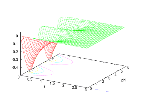
FIG. 1.: Smallest eigenvalue of $\rho^{T_{A}}$ as a function of $f$ and $\varphi$

Let me finally propose a concrete system where the effect might in principle be observable. Consider two double–well quantum dots enclosed in an ideally conducting, box–shaped cavity, with edge dimensions $a$, $b$, and $c$ in $x$, $y$, and $z$ directions, respectively. The two quantum dots are assumed identical, with the two–dimensional electron gas in the $y=b/2$ plane, and with two identical wells to the right and left (in $z$ direction) each, which might be electrostatically defined by suitable gate–electrodes. The symmetry centers of the double–well quantum dots are located at ${\bf x}_{A}=(a/4,b/2,c/2)$ and ${\bf x}_{B}=(3a/4,b/2,c/2)$ for dot $A$ and $B$, respectively. The centers of the wells are separated by a distance $d$ and we will assume that there exist in both dots two states $|0\rangle$ and $|1\rangle$, localized in the right and left well, such that they are eigenstates of the dipole operators, i.e. $e{\bf r}_{A}$, $\langle 0|{\bf r}_{A}|0\rangle=-d/2(0,0,1)=-\langle 1|{\bf r}_{A}|1\rangle$, $\langle 0|{\bf r}_{A}|1\rangle=0$ for dot $A$, where $e$ is the electron charge and ${\bf r}_{A}={\bf x}-{\bf x}_{A}$ is the position of an electron with respect to the center of the dot. This can be achieved to very good approximation by a very high barrier between the two wells, which leads to exponentially small overlap of the two wave functions, and negligible tunneling splitting. For dot $B$ the two states are chosen in the opposite way, $\langle 0|{\bf r}_{B}|0\rangle=d/2(0,0,1)=-\langle 1|{\bf r}_{B}|1\rangle$. The cavity supports TE and TM modes (“transversal” relative to the arbitrarily chosen $z$–direction as propagation direction). For the above geometry the two dots interact only with the TM modes, if we describe the interaction between the dots and the electromagnetic field in dipole approximation. This is suitable for temperatures where only modes with wave lengths much larger than $d$ are populated, i.e. $k_{B}T\ll 2\pi\hbar c_{0}/d$ ($c_{0}$ is the speed of light). The interaction in dipole approximation reads

$$H_{\rm int}^{A,B} = -\sum_{i,j=0}^{1}P_{i,j}^{A,B}|i\rangle\langle j|\sum_{{\bf k}}{\cal E}_{{\bf k}}({\bf x}_{A,B})\hat{q}_{{\bf k}}\,,$$ (13)

where $P_{i,j}^{A,B}=e\langle i|{\bf r}_{A,B}|j\rangle$ are the dipole matrix elements defined above, ${\cal E}_{{\bf k}}=\sqrt{\frac{m}{2\mu_{0}}}(\varphi_{x},\varphi_{y},\varphi_{z})$ (with $\epsilon_{0}$ and $\mu_{0}$ electric permeability and magnetic susceptibility of vacuum, in SI units), and $\hat{q}_{\bf k}$ is the electric field amplitude of mode ${\bf k}$ with the dimension of a length, chosen as coordinate of the harmonic oscillator in the quantization of the field [19]. The mass $m$ introduced formally for this purpose will cancel out again in the final expressions for $f(t)$ and $\varphi(t)$. The functions $\varphi_{x}$, $\varphi_{y}$, and $\varphi_{z}$ define the spatial structure of the modes. Here, only $\varphi_{z}$ is needed, which for perfectly conducting walls is given by [20]

$$\varphi_{z}({\bf x})=-\frac{2\sqrt{2}}{\sqrt{V}}\frac{k_{\perp}}{\epsilon_{0}}\sin(k_{x}x)\sin(k_{y}y)\cos(k_{z}z)\,;$$ (14)

$V=abc$ denotes the total volume, $k_{\perp}=\sqrt{k_{x}^{2}+k_{y}^{2}}$ are the transverse wave numbers, and the wave vector is given by $(k_{x},k_{y},k_{z})=\pi(m/a,n/b,p/c)$, $m,n,p=0,1,2,\ldots$. Thus,

$$H_{\rm int}^{A,B} = \mp\sigma_{x}^{A,B}\sum_{{\bf k}}g_{{\bf k}}^{A,B}\hat{q}_{{\bf k}}\,,$$ (15)

$$g_{{\bf k}}^{A} = ed\sqrt{\frac{m}{\mu_{0}V}}\frac{k_{\perp}}{\epsilon_{0}}\sin(k_{x}\frac{a}{4})\sin(k_{y}\frac{b}{2})\cos(k_{z}\frac{c}{2})$$ (16)

$$g_{{\bf k}}^{B} = ed\sqrt{\frac{m}{\mu_{0}V}}\frac{k_{\perp}}{\epsilon_{0}}\sin(k_{x}\frac{3a}{4})\sin(k_{y}\frac{b}{2})\cos(k_{z}\frac{c}{2})\,.$$ (17)

The upper sign refers to dot $A$, the lower to $B$, and the operators $\sigma_{x}^{A,B}$ are defined for both systems as $\sigma_{x}=|0\rangle\langle 0|-|1\rangle\langle 1|$. One easily sees that the modes with even $m$ couple to $\sigma_{x}^{A}+\sigma_{x}^{B}$, those with odd $m$ couple to $\sigma_{x}^{A}-\sigma_{x}^{B}$. However, the odd modes can be suppressed by a very thin, uncharged, and perfectly conducting wire in the $z$ direction along the $x=a/2,y=b/2$ axis of the cavity, since they have non–vanishing tangential electrical field at the position of the wire. We then obtain the coupling Hamiltonian (3) with $S^{A}=\sigma_{x}^{A}$, $S^{B}=\sigma_{x}^{B}$, $g_{\bf k}=-g_{\bf k}^{A}$, and quantized wave vectors ${\bf k}=\pi((4n_{x}+2)/a,(2n_{y}+1)/b,2n_{z}/c)$, $n_{x},n_{y},n_{z}=0,1,2,\ldots$. The resulting expressions for $f(t)$ and $\varphi(t)$ are divergent, and the sum over ${\bf k}$ needs a cut–off. For a cavity made out of a real metal a natural cut–off frequency is the plasma frequency $\omega_{p}$, since the metal looses its reflectivity for $\omega>\omega_{p}$ [21]. Converting the sums over ${\bf k}$ into integrals, defining $\zeta(d,\beta)=e^{2}d^{2}\mu_{0}/(\pi^{2}c_{0}\hbar^{3}\beta^{2})$, and $\tau=\beta\hbar/2$, one finds $f(t)=\zeta(d,\beta)\tilde{f}(t)$ and $\varphi(t)=\zeta(d,\beta)\tilde{\varphi}(t)$ with

$$\tilde{f}(t) = \frac{1}{4}\int_{0}^{\infty}dx\,x\coth(x)\,c(x)\left(1-\cos\frac{xt}{\tau}\right)$$ (18)

$$\tilde{\varphi}(t) = \frac{1}{3}\int_{0}^{\infty}dx\,x^{2}c(x)\left(\frac{xt}{\tau}-\sin\frac{xt}{\tau}\right)\,,$$ (19)

where $c(x)$ is a cut-off function (to be specific, say $c(x)=\exp(-x/x_{\rm max})$) For an aluminum cavity, $\hbar\omega_{p}=15.3$eV [21], and we have, at $T=100$mK, $\tau\simeq 3.8\,10^{-11}$s and $x_{\rm max}=\omega_{p}\tau\simeq 8.8\,10^{5}$. The main contribution to the integrals therefore stems from $x\gg 1$, where we can approximate the coth–function by 1. For the exponential cut–off we then have

$$\tilde{f}(t)=x_{\rm max}^{2}\left(1-\frac{\cos\left(2\arctan(tx_{\rm max}/\tau)\right)}{1+t^{2}x_{\rm max}^{2}/\tau^{2}}\right)\,,$$ (20)

a function that saturates for $tx_{\rm max}\gg\tau$ at the value $x_{\rm max}^{2}$, after reaching a maximum at $t/\tau\simeq x_{\rm max}^{-1}$ . For quantum dots with $d=10$nm, $T=100$mK, $\zeta(d,\beta)\simeq 1.8\,10^{-15}$, and $f(t)$ reaches a maximum after a time of the order $10^{-17}$s before saturating at $f(t)\simeq 0.0014$. This means that decoherence remains incomplete even for non–symmetric couplings, and the entanglement created by the interaction with the heat bath is preserved, till other decoherence mechanisms neglected in the above analysis kick in. Note that such incomplete decoherence is a rather general result for systems with degenerate energy levels. In fact, by integrating the time dependent part in eq.(18) from zero to $t$ one obtains for $t\to\infty$ a Dirac delta function at $x=0$, and the remaining integral over $x$ will give a finite constant. Thus, the time dependent part of $\tilde{f}(t)$ has to decay for $t\to\infty$ faster than $1/t$, leaving the time independent part $\int dx\,x\coth(x)c(x)/4$. Note that the factor $x$, the spectral weight of the heat bath at zero frequency, is essential in this reasoning. Decoherence will always remain incomplete (in the sense of finite $f(t)$ for $t\to\infty$, depending on the circumstances even $f(t)\ll 1$) between degenerate energy levels for spectral weights that vanish at zero frequency faster than the first power of the frequency.

The presented scheme has an advantage over conventional creation of entanglement if Alice and Bob are so far apart that a direct interaction is difficult to achieve. Since $f(t)$ and $\varphi(t)$ do not depend on the volume of the cavity, very large cavities should be possible with corresponding large distances between Alice and Bob; using the non–symmetric coupling scheme one might even envisage to dispose of the cavity altogether and rely on the long wave–length continuum of the cosmic electromagnetic background radiation to create entanglement between very remote quantum dots. While only a small amount of mixed state entanglement will be created, it is well known that all entanglement of a $2\times 2$ bipartite system can be distilled into a pure entangled state [22], given sufficiently many realizations of the input states and local coherent control.

As a conclusion I have shown that entanglement can be created between two qubits that interact solely with a common heat bath with very many degrees of freedom. The explicit example of two double–well quantum dots in a cavity was calculated, and the phenomena of “incomplete decoherence” was revealed, which may, as much as symmetric couplings to the environment, preserve the entanglement created by the heat bath.

Acknowledgements: I would like to thank Fritz Haake and Walter Strunz for many discussions on decoherence.

REFERENCES

- [1] E. Schroedinger, Die Naturwissenschaften, 23, 807 (1935).
- [2] C.H. Bennett et al., Phys. Rev. Lett. 69, 2881 (1992).
- [3] C.H. Bennett et al., Phys. Rev. Lett. 70, 1895 (1993).
- [4] R. Jozsa and N. Linden, quant-ph/0201143.
- [5] J.I. Cirac and P. Zoller, Phys. Rev. Lett. 74, 4091 (1995); A.M. Steane, Appl. Phys. B, 64, 623 (1997); C. Monroe, D.M. Meekhof, B.E. King, W.M. Itano, and D.J. Wineland, Phys. Rev. Lett. 75, 4714 (1995).
- [6] P. Domokos, J.M. Raimond, M. Brune, and S. Haroche, Phys. Rev. A, 52, 3554 (1995).
- [7] A. Beige, D. Braun, B. Tregenna, and P.L. Knight, Phys. Rev. Lett. 85, 1762 (2000).
- [8] R. Bonifacio, P. Schwendiman, and F. Haake, Phys. Rev. A 4, 302 (1971); M. Gross and S. Haroche, Phys. Rep. 93, 301 (1982); P.A. Braun, D. Braun, and F. Haake, Eur. Phys. J. D 3, 1 (1998).
- [9] S. Schneider and G.J. Milburn, quant-ph/0112042.
- [10] W.H. Zurek, Phys. Rev. D, 26, 1862 (1982); E. Joos and H.D. Zeh, Z.Phys B 59, 223 (1985).
- [11] W.H. Zurek, Phys. Rev. D 26, 1862 (1982).
- [12] K.H. Stevens, J. Phys. C 16, 5765 (1983); D. Braun and U. Weiss, Z. Phys. B 92, 507 (1993).
- [13] D. Braun, P. A. Braun, and F. Haake, Opt. Comm. 179, 411, (2000).
- [14] D.A. Lidar, I.L. Chuang, and K.B. Whaley, Phys. Rev. Lett. 81, 2594 (1998).
- [15] D. Braun, Dissipative Quantum Chaos and Decoherence, Springer Tracts in Modern Physics 172 (Springer, Berlin, 2001).
- [16] M. A. Nielsen and I. L. Chuang, Quantum Computation and Quantum Information, Cambridge University Press, Cambridge, UK (2000).
- [17] M. Horodecki, P. Horodecki, and R. Horodecki, Phys. Lett. A, 223, 1 (1996).
- [18] D. Braun, F. Haake, and W.T. Strunz, Phys. Rev. Lett. 86, 2913 (2001).
- [19] M.O. Scully and M.S. Zubairy, Quantum Optics, Cambridge University Press, Cambridge, UK (1997).
- [20] J.D. Jackson, Classical Electrodynamics 2nd ed., John Wiley and Sons, New York (1975).
- [21] Ch. Kittel, Introduction to Solid State Physics, 6th ed., John Wiley and Sons, Inc. New York (1986).
- [22] M. Horodecki, P. Horodecki, and R. Horodecki, Phys. Rev. Lett. 78, 574 (1997).