Simulation of Markovian quantum dynamics on quantum logic networks

Abstract

We study how generators of Markovian dynamics of a qubit can be simulated using a programmable quantum processor.

I Introduction

Quantum computing offers a new perspective in simulating physical systems[1, 2]. While the simulation of a larger quantum system is intractable for a classical computer, it should be possible of course on a quantum computer. Quantum computers are, from a theoretical point of view, highly simplified quantum systems. A simulation of a real physical system on such an arrangement is therefore also interesting necessarily because of the usefulness of the simulation result, but also because it may reveal fundamental aspects of the real physical system, which may be obscure otherwise.

Maybe the most general problem of this kind would be the simulation of general quantum operations[3], the most general dynamics a quantum system can undergo. The idea is to represent the initial state of the system on a quantum bit array, and supplement it with another array embodying the environment. Subjecting this system to the effect of a quantum logic network, and dropping the environment bits, the resulting state of the data should be obtained. Naturally, having infinite resources, i.e. arbitrary number of “environment” bits, any operation can be carried out by realizing a unitary representation of the process. For a system with a $k$ dimensional Hilbert space, this requires a $k^{2}$ dimensional environment. Lloyd conjectured [4], that a general quantum operation on a system with a $k$ dimensional Hilbert-space can be simulated with a $k$-dimensional environment, which may be in a mixed sate initially. This conjecture was falsified by Terhal et al. [5], who give bounds to the dimensionality of the environment required to simulate certain quantum operations on a single qubit system. Zalka and Rieffel[6] give a simpler proof via explicit construction of counterexamples. More optimal possibilities for the simulation, such as closed loop schemes were discussed in detail in Refs. [7, 8].

Programmable quantum gate arrays or quantum processors [9, 10, 11, 12] provide another possible approach to the problem. In this case, the parameters of the dynamics should be stored in the initial state of the “environment” (which play a role of the “program register” - see below). The quantum processor has two input registers, one storing the state of the system to be simulated (the “data register”), while the other contains the data of the operation to be performed. After the operation of the circuit, the remains of the program state in the program register may either be dropped or be subjected to a measurement. The latter is the probabilistic regime of the quantum processor. The result is accepted, if the measurement yields a given result. It was shown by Hillery et al. [11, 12], that in this case, any operation can be implemented, though some of them with quite low probability of success. Recently Vidal et al. [13] have presented a probabilistic scheme implementing unitary transformations with rather high probability.

In this paper we restrict ourselves to the “deterministic” case, that is, the remains of the program register are dropped. Hillery et al. [14] have studied the possibility of implementing general quantum maps in such a scheme. They have shown, that there are certain limitations, e.g., an amplitude damping channel cannot be implemented. In addition to this, we show that different quantum circuits such as quantum teleportation [15] can be used as a programmable quantum circuit for some purpose, as it is related to a phase damping channel [16].

We focus here on a specific subset of quantum operations, namely Markovian dynamics. These processes are the most important ones in the description of quantum decoherence. The question of simulating Markovian dynamics in the quantum computing context was investigated by Bacon et al. [17]. As one of their main results, these authors provide a decomposition rule to build more complex dynamics from simpler “primitive” operations. On the other hand, Bacon et al. apply the formalism of Gorini, Kossakowski and Sudarshan (GKS) [18], providing an excellent framework for the treatment of Markovian processes. We approach the problem of simulating Markovian dynamics differently in a way that is related to programmable quantum gate arrays. We restrict ourselves to single qubit dynamics, with a single qubit program register. We intend to simulate the generator of Markovian dynamics on a programmable quantum logic array, as the generator characterizes the time evolution completely in this case. A single run of the processor simulates an infinitesimal time step. As a further restriction we require that the length infinitesimal time step should be encoded into the initial state of the program register.

The paper is organized as follows: in Section II we review some definitions concerning Markovian dynamics, introducing Lindbladians, the generators of the dynamics. The standard GKS matrix-representation introduced by Gorini, Kossakowski and Shudarsan in Ref. [18] is reviewed, and a practical recipe is given for finding the GKS matrix from of a Lindbladian operator in the one-qubit case, utilizing the affine representation. In Section III we describe the general idea of simulating a generator, as understood in this paper. Section IV describes a reversible scheme capable of simulating a phase damping channel about an arbitrary axis. A geometrical interpretation of the result is also given. In Section V we discuss an application of Bennett’s teleportation scheme in this context. In section VI the results are summarized and conclusions are drawn.

II Markovian dynamics of a qubit

In this Section we review the definition of Markovian semigroup and its generators very briefly. The most general operation, that a state of a qubit can undergo is described by a completely positive linear, trace preserving map acting on the set of density operators, also called a superoperator. This may be written in the Krauss-representation[3] as

$${\cal{E}}(\varrho)=\sum\limits_{k}E_{k}\varrho E_{k}^{\dagger}$$ (1)

where the $E_{k}$-s are positive operators such that $\sum E_{k}^{\dagger}E_{k}=1$.

In order to introduce Markovian processes, one equips the set of superoperators with a continuous parameter $t$ which is called the time. Stationary and Markovian dynamics obey the property

$${\cal{E}}_{t_{1}}{\cal{E}}_{t_{2}}={\cal{E}}_{t_{1}+t_{2}},$$ (2)

with $t_{1},t_{2}>0$. The set of superoperators with property (2) form a one-parameter semigroup, the Markovian semigroup. We also require the property

$${\cal{E}}_{0}=\hat{1},$$ (3)

(where $\hat{1}$ stands for the identity superoperator) to hold.

The property in Eq. (2) enables us to define the generators of the semigroup as

$$\hat{L}(\varrho)=\lim\limits_{t\to 0+0}\frac{{\cal{E}}_{t}(\varrho)-\varrho}{t}.$$ (4)

The operator $\hat{L}$ is the infinitesimal generator of the time evolution:

$${\cal{E}}_{t}=\exp(\hat{L}t)=\lim\limits_{n\to\infty}\left(\hat{1}-\frac{t}{n}\hat{L}\right)^{-n},$$ (5)

from which follows, that

$$\frac{\partial\varrho(t)}{\partial t}=\hat{L}[\varrho(t)]$$ (6)

known as the master equation.

Let us consider an operator $\hat{L}$ acting on the Hilbert space of a qubit. The question arises, under what condition can this operator represent a generator of the dynamical semigroup. The answer was given by Lindblad [19], and by Gorini, Kossakowski and Sudarshan (GKS) [18]. We use the notation of the latter authors. According to this, the most general form of a generator of a Markovian semigroup reads

$${\hat{L}}(\varrho)=-i[\hat{H},\varrho]+\frac{1}{2}\sum\limits_{i,j=1}^{3}C_{i,j}([\hat{\sigma}_{i}\varrho,\hat{\sigma}_{j}]+[\hat{\sigma}_{i},\varrho\hat{\sigma}_{j}]),$$ (7)

where the $\hat{\sigma}$-s are the Pauli-matrices. The first contribution on the right hand size describes a possible unitary evolution, the Hamiltonian $\hat{H}$ being a Hermitian matrix which can be chosen to be traceless without the loss of generality. The second contribution describes the stochastic part of the evolution. The Hermitian positive semidefinite matrix $C_{i,j}$ is called the GKS matrix, and it contains all the information on the nature of the dynamics. Note that in order to preserve the trace of the density matrix, $\hat{L}\varrho$ should be traceless. In fact, Eq. (7) describes the most general linear operator taking $\varrho$ to a traceless matrix.

In the following we describe how to extract the Hamiltonian $\hat{H}$ and the GKS matrix $C$, if one is given an arbitrary function of a single-qubit density matrix $\varrho^{\prime}=\hat{L}\varrho$ In order to do so we utilize the relation between the GKS matrix and the affine representation described also in  [17].

A generic density matrix can be expanded on the basis of the three Pauli-matrices and the unit operator, obtaining its usual real 3-vector representation $\underline{r}$ displayable on the unit radius Bloch sphere:

$${\underline{r}}=\begin{pmatrix}r_{1}\cr r_{2}\cr r_{3}\end{pmatrix},\quad r_{i}=\mathop{\mbox{tr}}\nolimits(\varrho\hat{\sigma}_{i})\;,$$ (8)

so that

$$\varrho=\frac{1}{2}\left(\hat{1}+\sum\limits_{i=1}^{3}r_{i}\hat{\sigma}_{i}\right)\;.$$ (9)

Direct calculation shows that the real 3-vector $\hat{L}[\underline{r}]$ corresponding to the most general $\hat{L}\varrho$ in Eq. (7) reads

$$\hat{L}[\underline{r}]=\begin{pmatrix}0&-h_{3}&h_{2}\cr h_{3}&0&-h_{1}\cr-h_{2}&h_{1}&0\end{pmatrix}\underline{r}+\begin{pmatrix}-2(C_{22}+C_{33})&C_{12}+C_{21}&C_{13}+C_{31}\cr C_{12}+C_{21}&-2(C_{11}+C_{33})&C_{23}+C_{32}\cr C_{13}+C_{31}&C_{23}+C_{32}&-2(C_{11}+C_{22})\end{pmatrix}\underline{r}+2i\begin{pmatrix}C_{23}-C_{32}\cr C_{31}-C_{13}\cr C_{12}-C_{21}\end{pmatrix},$$ (10)

where

$$\hat{H}=\frac{1}{2}\sum\limits_{i=1}^{3}h_{i}\hat{\sigma}_{i}.$$ (11)

Thus $\hat{L}$ appears as an affine linear mapping in the 3 space, the above mapping is called the affine representation of $\hat{L}$.

If we are now given an arbitrary function $\varrho^{\prime}$, which is traceless and depends on the components of the arbitrary density matrix $\varrho$ linearly, we can find the corresponding $\underline{r^{\prime}}$ according to Eq. (8) as a function of the components of $\underline{r^{\prime}}$ representing $\varrho$. This is a linear inhomogenous operator, which can be always decomposed into a sum of a homogenous antisymmetric operator, a homogenous symmetric operator and a vector representing the inhomogenity. For qubits, this decomposition of the affine representation of the generator is quite meaningful: according to Eq. (10), the information on the unitary part of the generator, i.e. the Hamiltonian is encoded into the antisymmetric part of this operator, while the real and imaginary parts can be found from the symmetric part and the inhomogenity respectively.

In the absence of the inhomogenity the generator is zero for the identity operator:

$$\hat{L}\hat{I}=0,$$ (12)

thus it describes a unital evolution, which preserves the identity operator. The inhomogenity appears in the complex part of the elements of the GKS matrix: for qubits, real GKS matrices correspond to unital dynamics.

Thus equipped with Eq. (10), we have the recipe how to find the standard GKS form of a generator of a dynamical semigroup for a quantum bit.

III Simulation of infinitesimal generators

We intend to simulate the infinitesimal generator $L\hat{\varrho}$ of Markovian dynamics, on a single quantum bit. This can be understood in several ways. As an elementary step we consider the application of a quantum processor: an arrangement of quantum logic gates, and possibly measurements, acting on the qubit in argument, and certain ancillary systems. The ancillary systems can be used as a “program register”: their state can influence the action of the processor on the qubit in argument, which constitutes a “data bit” in this context.

The next question might be, how to interpret the time. A possible generic approach would be to regard the single run of the processor as a finite time step $\Delta t$. The repeated application of the processor on the data bit results then in a discrete time evolution. One can then examine if this is a stroboscopic version of some valid continuous time evolution, and search for the proper master equation. This approach will be discussed elsewhere. Here we adopt a simpler interpretation: we expect a single run of processor to simulate an infinitesimal time step:

$$\varrho_{\text{out}}=\varrho_{\text{in}}+\hat{L}\varrho_{\text{in}}dt+{\mathcal{O}}(dt^{2}),$$ (13)

where $dt$ should be encoded in the $|\Psi_{\text{prog}}\rangle$ of the program register. The entire evolution can then be approximated with some accuracy by running this process many many times. This implements the equidistant first order Euler method[20] of solving Eq. (6), but time step, and thereby the accuracy is encoded quantum mechanically. Of course, the simulation is completely accurate if $dt\to 0$, and the number of repetitions tends to infinity. We remark here, that simulation of decoherence mechanisms with an array of quantum gates has proven to be fruitful in other problems too [21, 22].

Physically, the simulation scheme can be envisaged as a simple collision model: The data qubit is represented by a physical system localized in space. It interacts with flying program bits represented by e.g. spin of particles emerging from an oven. Each program bit causes the system to evolve a small time step further.

It follows from Eq. (13), that there must exist a program state, for which $dt=0$, and thus $\varrho_{\text{out}}=\varrho_{\text{in}}$, in the quantum processor terminology we would say the processor implements the unit operator. It is a natural requirement for this kind of semigroup simulation. Thus our scheme is to some extent similar to the idea of simulating a reservoir with beam-splitters of transmittance around unity in quantum optics [23] or a quantum homogenization processes as described in Ref. [22].

IV A scheme without a measurement

First we consider a simple deterministic scheme with a single ancillary qubit, as depicted in Fig. 1.

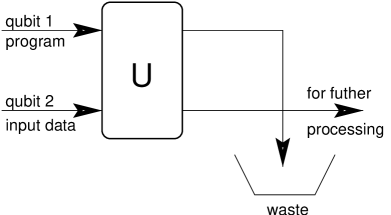
FIG. 1.: The quantum network for the deterministic scheme. A single run of the network simulates an infinitesimal time-step in the evolution.

The first bit contains the program, which is most generally

$$|\Psi_{\text{prog}}\rangle=\sqrt{1-\varepsilon}e^{i\chi}|0\rangle+\sqrt{\varepsilon}|1\rangle,\quad 0\leq\varepsilon\leq 1,\ \chi\ \text{real}.$$ (14)

We don’t consider mixed program states here, we want to study how decoherence associated with Markovian processes appears purely quantum-mechanically, and a mixed program state would imply some prescribed classical stochasticity. The input data is in bit 2, in the state $\varrho_{\text{in}}$. After the operation of the processor, the contents of the program register are dropped, and bit 2 contains the output

$$\varrho_{\text{out}}=\mathop{\mbox{Tr}}\nolimits_{1}\left(\hat{U}(|\Psi_{\text{prog}}\rangle\langle\Psi_{\text{prog}}|\otimes\varrho_{\text{in}})U^{\dagger}\right)$$ (15)

which is passed for further processing.

To have the identity operator implemented, there should be a program state for which $\varrho_{\text{out}}=\varrho_{\text{in}}$ holds. We chose this to be the program state $|0\rangle$. The most general processor that is possible under such circumstances is a controlled U gate:

$$\hat{U}=\begin{pmatrix}\hat{1}&0\cr 0&\hat{U}_{2}\end{pmatrix}$$ (16)

The lower right corner is an $SU(2)$ block:

$$\hat{U}_{2}=\begin{pmatrix}\cos(\frac{\theta}{2})e^{-i\frac{\phi+\psi}{2}}&-\sin(\frac{\theta}{2})e^{-i\frac{\phi-\psi}{2}}\cr\sin(\frac{\theta}{2})e^{i\frac{\phi-\psi}{2}}&\cos(\frac{\theta}{2})e^{i\frac{\phi+\psi}{2}}\end{pmatrix},$$ (17)

where we use the standard Euler angle parametrization in the $y$ convention [24].

Now we can evaluate Eq. (13) with a generic input data state of Eq. (9), and program of Eq. (14), to obtain the effect of a single run of the processor. Note that due to the orthogonality of the program states corresponding to $\hat{1}$ and $\hat{U}_{2}$ (which is a consequence of the unitarity of $\hat{U}$), Eq. (15) simplifies to

$$\varrho_{\text{out}}=(1-\varepsilon)\varrho_{\text{in}}+\varepsilon\hat{U}_{2}\varrho_{\text{in}}\hat{U}_{2}^{\dagger}.$$ (18)

Thus from the point of view of the effect on the input state, the quantum circuit does nothing else than apply the unitary operation $\hat{U}_{2}$ on the input state, with the probability $\varepsilon$. The difference is that if the operation is realized by the quantum circuit, then the information which disappears from the system will be stored in the dropped quantum state of the program register. In the other case the information will be entirely classical, one bit per infinitesimal timestep: we can be aware, whether the operation $\hat{U}_{2}$ was carried out or not. Note that in both of the cases the process is reversible, provided that we have the appropriate information at hand.

According to Eq. (18), we can write

$$\varrho_{\text{out}}=\varrho_{\text{in}}+(\hat{U}_{2}\varrho_{\text{in}}\hat{U}_{2}^{\dagger}-\varrho_{\text{in}})\varepsilon.$$ (19)

Thus we identify $\varepsilon=dt$, and comparing with Eq. (13) we get

$$\hat{L}\varrho_{\text{in}}=\hat{U}_{2}\varrho_{\text{in}}\hat{U}_{2}^{\dagger}-\varrho_{\text{in}}.$$ (20)

The transformation on the Bloch ball corresponding to $\hat{U}_{2}\varrho\hat{U}_{2}^{\dagger}$ is a rotation of the vector $\underline{r}$ corresponding to $\varrho$

$$\underline{r}^{\prime}={\mathcal{R}}(\theta,\phi,\psi)\underline{r},$$ (21)

where ${\mathcal{R}}$ is the appropriate element of the adjoint representation of $SU(2)$:

$${\mathcal{R}}(\theta,\phi,\psi)=\begin{pmatrix}-\sin\phi\sin\psi+\cos\theta\cos\phi\cos\psi&-\cos\theta\cos\phi\sin\psi-\sin\phi\cos\psi&\sin\theta\cos\phi\cr\cos\theta\sin\phi\cos\psi+\cos\phi\sin\psi&\cos\phi\cos\psi-\cos\theta\sin\phi\sin\psi&\sin\theta\sin\phi\cr-\sin\theta\cos\psi&\sin\theta\sin\psi&\cos\theta\end{pmatrix}\in SO(3)\;.$$ (22)

For the generator in Eq. (20) we have thus

$$\hat{L}[\underline{r}]=\left({\mathcal{R}}(\theta,\phi,\psi)-\hat{1}\right)\underline{r}.$$ (23)

This can be compared with Eq. (10) to extract the properties of the generator. The transformation in Eq. (23) is homogenous, thus the generated dynamics is unital.

As for the coherent part of the evolution, we get the Hamiltonian

$$\hat{H}=\begin{pmatrix}\sin(\phi+\psi)\cos^{2}\frac{\theta}{2}&-\frac{i}{2}\sin\theta\left(e^{-i\phi}+e^{i\psi}\right)\\ \frac{i}{2}\sin\theta\left(e^{i\phi}+e^{-i\psi}\right)&-\sin(\phi+\psi)\cos^{2}\frac{\theta}{2}\end{pmatrix}$$ (24)

This is zero if $\phi+\psi=(2k+1)\pi$ or $\theta=\pi+2k\pi$ holds, which is equivalent to $\mathop{\mbox{tr}}\nolimits U_{2}=0$. Thus in case of traceless unitaries, we obtain a purely stochastic evolution in the sense that it lacks the Hamiltonian part.

Evaluating the symmetric part of Eq. (22), and comparing with (10), we obtain the GKS matrix

$$C_{\theta,\phi,\psi}=\begin{pmatrix}\sin^{2}\frac{\theta}{2}\sin^{2}\frac{\phi-\psi}{2}&\frac{1}{2}\sin^{2}\frac{\theta}{2}\sin(\psi-\phi)&\frac{1}{4}\sin\theta(\cos\phi-\cos\psi)\cr\frac{1}{2}\sin^{2}\frac{\theta}{2}\sin(\psi-\phi)&\sin^{2}\frac{\theta}{2}\cos^{2}\frac{\phi-\psi}{2}&\frac{1}{4}\sin\theta(\sin\phi+\sin\psi)\cr\frac{1}{4}\sin\theta(\cos\phi-\cos\psi)&\frac{1}{4}\sin\theta(\sin\phi+\sin\psi)&\cos^{2}\frac{\theta}{2}\sin^{2}\frac{\phi+\psi}{2}\end{pmatrix}$$ (25)

Specifically, if $\hat{U}_{2}$ is traceless because $\psi=\pi-\phi$ holds, we obtain from Eq. (25) the following GKS matrix:

$$C_{\theta,\phi}=\begin{pmatrix}\sin^{2}\frac{\theta}{2}\cos^{2}\phi&\frac{1}{2}\sin^{2}\frac{\theta}{2}\sin(2\phi)&\frac{1}{2}\sin\theta\cos\phi\cr\frac{1}{2}\sin^{2}\frac{\theta}{2}\sin 2\phi&\sin^{2}\frac{\theta}{2}\sin^{2}\phi&\frac{1}{2}\sin\theta\sin\phi\cr\frac{1}{2}\sin\theta\cos\phi&\frac{1}{2}\sin\theta\sin\phi&\cos^{2}\frac{\theta}{2}\end{pmatrix}$$ (26)

The matrix in Eq. (26) can be interpreted as follows. Consider a unitary operator ${\mathcal{U}}\in SU(2)$ acting on the qubit’s Hilbert space, and a superoperator ${\mathcal{E}}$, which describes unitary evolution described by the GKS matrix $C$. According to Ref. [17] unitary conjugation of a superoperator ${\mathcal{E}}$, that is,

$${\mathcal{E}}^{\prime}={\mathcal{U}}^{\dagger}{\mathcal{E}}{\mathcal{U}},$$ (27)

where ${\mathcal{U}}(\varrho)={\mathcal{U}}\varrho{\mathcal{U}}^{\dagger}$ yields another superoperator describing Markovian dynamics as well. The resulting GKS matrix is

$$C^{\prime}={\mathcal{R}}C{\mathcal{R}}^{T},$$ (28)

where ${\mathcal{R}}$ is the element of $SO(3)$, the adjoint representation of $SU(2)$ corresponding to $\mathcal{U}$, and the $T$ stands for transposition. Thus $\mathcal{R}$ is a real 3-rotation, which can be visualized as a rotation in the Bloch-sphere picture. The effect of unitary conjugation is to apply the same operation on a transformed basis. In the actual case, the matrix in Eq. (26) can be rewritten as

$$C_{\theta,\phi}={\mathcal{R}}(\theta/2,\phi,\psi)\begin{pmatrix}0&&\cr&0&\cr&&1\end{pmatrix}{\mathcal{R}}^{T}(\theta/2,\phi,\psi).$$ (29)

The matrix between the two rotations defines a phase damping about the $z$ axis. Thus the process is a phase damping about an axis pointing towards the spherical polar angles $\theta/2,\phi$. In fact the rotation $U_{2}$ moves the $z$ axis to the direction described by the spherical polar angles $\theta/2,\phi$, so the direction of the phase damping is “half way” between the $z$ axis, and its transform by $U_{2}$. Note that the angle $\psi$ is irrelevant in Eq. (29), as it does not influence the polar angle of the rotated $z$ axis. The phase damping channel has a single direction which is special, thus it is necessarily described by two parameters. In the case if $\hat{U}_{2}$ is traceless because $\theta=\pi+2k\pi$ is satisfied, we obtain a phase damping channel about an axis in the $xy$ plane. We can conclude that the controlled-U gate with a traceless $U_{2}$ is capable of simulating a generator of an arbitrary phase damping channel in our scheme.

Returning to the generic GKS matrix in Eq. (25) we find that $\mathop{\mbox{rank}}\nolimits C_{\theta,\phi,\psi}=1$, thus this general GKS matrix also describes a phase damping channel, physically the same process as in the traceless case. The only difference is that the evolution is now accompanied by a coherent part, generated by the Hamiltonian in Eq. (24).

V Control via teleportation

In this Section we briefly describe another simulation scheme based on Bennett’s quantum teleportation. It is depicted in Fig. 2

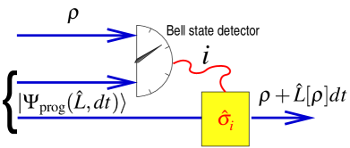
FIG. 2.: Bennett’s teleportation scheme as a programmable circuit for Markovian decoherence

The initial state $\varrho$ impinges at the input of a teleportation arrangement. Two additional qubits are prepared in an entangled state

$$|\Psi_{\text{prog}}\rangle=\sqrt{1-\varepsilon}|B_{0}\rangle+\sqrt{\varepsilon}\left(\alpha_{1}|B_{1}\rangle+\alpha_{2}|B_{2}\rangle+\alpha_{3}|B_{3}\rangle\right),$$ (30)

with $|\alpha_{1}|^{2}+|\alpha_{2}|^{2}+|\alpha_{3}|^{2}=1$, which serves as the program state. We use the notation

$$|B_{0}\rangle=\frac{1}{\sqrt{2}}\left(|0\rangle|1\rangle-|1\rangle|0\rangle\right)\;;$$ (31)

$$|B_{1}\rangle=\frac{1}{\sqrt{2}}\left(|0\rangle|0\rangle-|1\rangle|1\rangle\right)\;;$$ (32)

$$|B_{2}\rangle=\frac{1}{\sqrt{2}}\left(|0\rangle|0\rangle+|1\rangle|1\rangle\right)\;;$$ (33)

$$|B_{3}\rangle=\frac{1}{\sqrt{2}}\left(|0\rangle|1\rangle+|1\rangle|0\rangle\right).$$ (34)

for the elements of the Bell basis. Then the usual Bennett teleportation is carried out: a Bell state measurement on the two appropriate qubits is carried out, and depending on the result, the appropriate unitary transformation $\hat{\sigma}_{i}$ (the identity operator or one of the Pauli operators) is carried out.

For $\varepsilon=0$ we have $|\Psi_{\text{prog}}\rangle=|B_{0}\rangle$, the state $\varrho$ is simply teleported: the identity operator is implemented. However, for nonzero $\varepsilon$ we obtain

$$\varrho^{\prime}=(1-\varepsilon)\varrho+\varepsilon\left(|\alpha_{1}|^{2}\hat{\sigma}_{1}\varrho\hat{\sigma}_{1}+|\alpha_{2}|^{2}\hat{\sigma}_{2}\varrho\hat{\sigma}_{2}+|\alpha_{3}|^{2}\hat{\sigma}_{3}\varrho\hat{\sigma}_{3}\right)$$ (35)

as a “teleported” state. Thus the scheme is essentially equivalent to a random application of the Pauli operators. Setting $dt=\varepsilon$ as in the previous Section, we can define

$$\hat{L}\varrho=|\alpha_{1}|^{2}\hat{\sigma}_{1}\varrho\sigma_{1}+|\alpha_{2}|^{2}\hat{\sigma}_{2}\varrho\sigma_{2}+|\alpha_{3}|^{2}\hat{\sigma}_{3}\varrho\sigma_{3}-\varrho.$$ (36)

A straightforward calculation shows that the corresponding GKS matrix reads

$${\mathcal{C}}(\alpha_{1},\alpha_{2},\alpha_{3})=\begin{pmatrix}|\alpha_{1}|^{2}&&\cr&|\alpha_{2}|^{2}&\cr&&|\alpha_{3}|^{2}\end{pmatrix}.$$ (37)

We have obtained a GKS matrix of rank 3, describing a generic Pauli channel. In this case we have the parameters of the dynamics encoded into the program state, too.

It is worth noting here that this second scheme is indeed irreversible. However, the same process could be simulated in a similar reversible framework as in Section IV, utilizing two ancillary qubits, and the universal programmable quantum gate array in Ref. [11, 12].

VI Summary

We have investigated quantum computational schemes for the simulation of a generator of Markovian dynamics on a qubit, where the value of the infinitesimal time step is encoded in a quantum state at the input of the device. We have described the capabilities of the arrangement if the ancilla to be applied is restricted to a single qubit by characterizing the most general Lindbladian that can be simulated. We have found that under these restrictions, a phase damping about an arbitrary axis can be simulated. We have also investigated a the Bennett quantum teleportation scheme as a possible quantum circuit for performing a similar task.

The inevitable advantage of this method compared with a classical simulation of quantum dynamics is that it works for any, even unknown initial state, which may emerge as an output of another quantum calculation.

The analysis can be carried out for systems ancillas of larger size but in that case, the number of parameters grows, and the problem is less transparent. We remark that for instance, the two-qubit program state enables non-unital dynamics as well.

We believe that the study of simple quantum systems such as those described here facilitates the understanding decoherence in general.

- [1] Yu. I. Manin, Vychislimoe i nevychislimoe, Sovetskoye Radio, Moscow, 1980.
- [2] R. P. Feynman, Int. J. Theor. Phys. 21, 467 (1982).
- [3] K. Krauss, States, Efffects and Operations: Fundamental Notions of Quantum Theory (Springer Verlag, Berlin, 1983).
- [4] S. Lloyd, Science 273, 1073 (1996).
- [5] B. M. Terhal et al., Phys. Rev. A 60, 881 (1999).
- [6] C. Zalka and E. Rieffel, J. Math. Phys. 43, 4376 (2002).
- [7] L. Viola, S. Lloyd, and E. Knill, Phys. Rev. Lett. 83, 4888 (1999).
- [8] S. Lloyd and L. Viola, Phys. Rev. A 65, 010101 (2002).
- [9] M. A. Nielsen and I. L. Chuang, Phys. Rev. Lett. 79, 321 (1997).
- [10] G. Vidal, L. Masanes, and J. Cirac, e-print (2001), quant-ph/0102037.
- [11] M. Hillery, V. Bužek, and M. Ziman, Fortschritte Phys.-Prog. Phys. 49, 987 (2001).
- [12] M. Hillery, V. Bužek, and M. Ziman, Phys. Rev. A 65, 022301 (2002).
- [13] G. Vidal, L. Masanes, and J. I. Cirac, Phys. Rev. Lett. 88, 047905 (2002).
- [14] M. Hillery, M. Ziman, and V. Bužek, Phys. Rev. A 66, 042302 (2002).
- [15] Ch. Bennett et al., Phys. Rev. Lett. 70 1895 (1993).
- [16] G. Bowen and S. Bose, Phys. Rev. Lett. 87 267901 (2001).
- [17] D. Bacon et al., Phys. Rev. A 64, 062302 (2001).
- [18] V. Gorini, A. Kossakowski, and E. C. G. Sudarshan, J. Math. Phys 17, 821 (1976).
- [19] G. Lindblad, Comm. Math. Phys. 48 119 (1976).
- [20] W. H. Press, S. A. Teukolsky, W. T. Vetterling, and B. P. Flannery, Numerical recipes in Fortran 77 (Cambridge University press, Cambridge, 1992).
- [21] V. Scarani et al., Phys. Rev. Lett. 88, 097905 (2002).
- [22] M. Ziman et al., Phys. Rev. A 65, 042105 (2002).
- [23] M. S. Kim and N. Imoto, Phys. Rev. A 52, 2401 (1995).
- [24] Eric W. Weisstein. ”Euler Angles.” From MathWorld–A Wolfram Web Resource. http://mathworld.wolfram.com/EulerAngles.html