Three-dimensional theory for interaction between atomic ensembles and free-space light

Abstract

Atomic ensembles have shown to be a promising candidate for implementations of quantum information processing by many recently-discovered schemes. All these schemes are based on the interaction between optical beams and atomic ensembles. For description of these interactions, one assumed either a cavity-QED model or a one-dimensional light propagation model, which is still inadequate for a full prediction and understanding of most of the current experimental efforts which are actually taken in the three-dimensional free space. Here, we propose a perturbative theory to describe the three-dimensional effects in interaction between atomic ensembles and free-space light with a level configuration important for several applications. The calculations reveal some significant effects which are not known before from the other approaches, such as the inherent mode-mismatching noise and the optimal mode-matching conditions. The three-dimensional theory confirms the collective enhancement of the signal-to-noise ratio which is believed to be one of the main advantage of the ensemble-based quantum information processing schemes, however, it also shows that this enhancement need to be understood in a more subtle way with an appropriate mode matching method.

I Introduction

Recently, many interesting schemes have been proposed which use atomic ensembles with a large number of identical atoms as the basic system for quantum state engineering and for quantum information processing. For instance, one can use atomic ensembles for generation of substantial spin squeezing [1, 2, 3] and continuous variable entanglement [4, 5, 6], for storage of quantum light [7, 8, 9, 10, 11], for realization of scalable long-distance quantum communication [12], and for efficient preparation of many-party entanglement [13]. The experimental candidates of atomic ensembles can be either some cold or ultracold atoms in a trap [2, 10], or a cloud of room-temperature atomic gas contained in a glass cell with coated walls [3, 6, 11]. The schemes based on atomic ensembles have some special advantages compared with the quantum information schemes based on the control of single  particles: firstly, laser manipulation of atomic ensembles without separate addressing of individual atoms is normally easier than the coherent control of single particles; Secondly, and more importantly, atomic ensembles with suitable level configurations could have some kinds of collectively enhanced coupling to certain optical mode (called the signal light mode) due to the many-atom interference effects. Thanks to this enhanced coupling, we can obtain collective enhancement of the signal-to-noise ratio (that is, the ratio between the controllable coherent interaction and the uncontrollable noisy interactions) compared with the single-particle case if we choose to manipulate the appropriate atomic and optical modes. This collective enhancement plays an important role in all the recent schemes based on the atomic ensembles.

To describe the interaction between atomic ensembles and optical beams, in particular, to understand the collective enhancement of the signal-to-noise ratio, normally one assumed a simple cavity-QED model [7, 8, 12, 1] or a one-dimensional light propagation model [9, 4] with an independent spontaneous emission rate for each atom. In contrast to this, most of the current experiments are done with free-space atomic ensembles coupling directly to the three-dimensional optical beams [3, 6, 10, 11]. It is not obvious that the predictions from the simple models will always be valid for this real much more complicate experimental situations. To fully predict and understand the real experiments, one needs to answer various questions associated with the three-dimensional interaction effects, for instance, what is the inherent mode structure of the signal light when we have a definite geometry of the atomic ensemble? Can we achieve a good mode matching with the matching efficiency in principle arbitrarily close to one? What is the noise magnitude associated with density fluctuation (induced by the random initial distribution of the atom positions and the random atomic motion) of the atomic ensemble? In the three-dimensional configuration, is there still the collective enhancement of the signal-to-noise ratio?

In this paper, we will try to provide answers to the above important questions for a Raman type $\Lambda$-level configuration which is useful for scalable long-distance quantum communication [12] and for many-party entanglement generation [13]. In general, it is very challenging to build a full quantum theory from the first principle to describe the interaction between the many-atom ensemble and the infinite-mode optical field and to give definite answers to the above-listed questions. In this paper, we will use a perturbative approach by assuming that the Raman pumping laser is very weak. There are several motivations to use a perturbative approach: firstly, the schemes in [12, 13] for scalable quantum communication and for many-party entanglement generation can work in the weak-pumping limit, so the perturbative approach describes a useful realistic situation. Secondly, the perturbative calculations allow us to investigate the three-dimensional effects and to give definite answers to the questions listed above from the first principle without any doubtful approximation. Finally, we expect the three-dimensional effects should be at least to some extent independent of the power of the pumping laser, so the perturbative calculations could give at least some indications for the three-dimensional interaction picture in other regions.

The calculations reveal some significant results which are unexpected from the simple models, for instance, it turns out that due to the density fluctuation of the atomic ensemble, there will be two sources of noise for the light-atomic-ensemble interaction: one is the spontaneous emission loss and the other is the inherent mode mismatching noise (here, by “inherent”, we mean that this mode mismatching is not from any technical imperfection). Thus, we need to use two quantities to describe the signal-to-noise ratios, and need to keep a balance between these two sources of noise by appropriate mode matching methods to optimize the setup for applications. The intuitive mode matching method will result in a quite large inherent mode mismatching noise. It is better to use some other mode matching methods which reduce the mode matching noise at the price of increasing the spontaneous emission loss. This can optimize the setup for some applications, such as the ones in Refs. [12, 13], since there the spontaneous emission loss has a far less important influence. The calculations in this paper also demonstrate that in the realistic three-dimensional configuration, one can still obtain large collective enhancement of the signal-to-noise ratio for atomic ensembles compared with the single-atom case, which is an important feature of this kind of systems.

It is also helpful to make a comparison between the collective enhancement of the signal-to-noise ratio we consider here and some other collective optical effects, such as the superradiance. The similarity lies in that both phenomena involve many-atom interference. However, there are also important differences. For superradiance, it is a stimulated emission effect, and the enhancement is in the emission speed. At the initial stage, coherence is built between different atoms from the spontaneous emissions. After the coherence has been built, superradiance can be understood even from a classical interference picture. For the light-atomic-ensemble interaction considered here, we are still completely in the spontaneous emission region which needs a full  quantum description, and the enhancement is not in the emission speed, but in the signal-to-noise ratio when we only manipulate and measure a definite atomic mode (called the symmetric collective atomic mode) and a definite signal light mode (which is the optical mode collinear with the Raman pumping light). The coupling between the above atomic and the optical modes are coherent for different atoms (which means for this coupling there is a certain phase relation between different atoms), while the coupling of these two modes to other atomic and other optical modes (called the noise modes) are inherent with random phase relations between different atoms (the randomness comes from the random atom positions). We have collective enhancement of the signal-to-noise ratio since the coherent coupling interferes constructively for different atoms. Of course, in the three-dimensional free-space, there are infinite optical modes, and the signal light mode changes continuously to other noisy optical modes when we continuously vary the solid angle. Due to the continuous change from the coherent coupling to the inherent coupling, we have non-trivial mode matching problem, and we get some inherent mode mismatching noise.

We also would like to mention that there are some early important works on the transverse effects of the Raman interaction by using the three-dimensional light propagation equations [14]. However, it is not clear to us how to use this approach to describe the collective enhancement of the signal-to-noise ratio, and in particular, how to give definite answers to the questions listed above. There is also some unpublished effort to try to figure out the three-dimensional effects in another light-atom interaction configuration [15]. The interaction picture is not yet clear to us.

This paper is arranged as follows: in Sec. II, we explain the interaction scheme and the basic ideas of the applications of this interaction scheme for quantum information processing. With the applications in mind, we can focus our efforts on the most relevant quantities that we need to calculate. We will also explain in this section the basic interaction picture between the light and the atomic ensemble from our calculations. Then, in the next section, we will describe the theoretical model for this light-atom interaction from the first principle, and solve this model by using a perturbative approach. In Sec. IV, we will discuss the properties of this solution, in particular, we will define and calculate the mode structure of the signal light, the spontaneous emission inefficiency, and the inherent mode mismatching noise. Sec. V is devoted to the discussion of the appropriate mode matching methods for real experiments. We show that by appropriate mode matching methods, we can keep a balance between the two sources of noise mentioned above in order to optimize this setup for applications. Finally, in Sec. VI we summarize the results.

II The interaction scheme and its applications

The basic element of our system is an atomic ensemble, which consists of a cloud of $N_{a}$ identical atoms with the relevant level structure shown in Fig. 1. A pair of metastable lower states $|g\rangle$ and $|s\rangle$ can correspond, for instance, to hyperfine or Zeeman sublevels of electronic ground state of alkali atoms. The relevant coherence between the levels $|g\rangle$ and $|s\rangle$ can be maintained for a long time, as has been demonstrated both experimentally [6, 10, 11] and theoretically [7, 8, 9]. All the atoms are initially prepared in the ground state $\left|g\right\rangle$ through optical pumping.

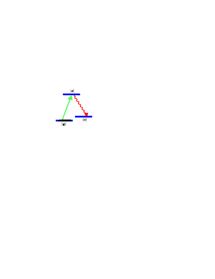
FIG. 1.: The relevant atomic level structure with $\left|g\right\rangle$,$\left|s\right\rangle$, a pair of ground or metastable states, and $\left|e\right\rangle$ , the excited state.

The ensemble is then illuminated by a weak pumping laser pulse which couples the transition $|g\rangle\rightarrow|e\rangle$ with a large detuning $\Delta$, and we look at the spontaneous emission light from the transition $|e\rangle\rightarrow|s\rangle$, whose polarization and/or frequency are assumed to be different to the pumping laser. There are two interaction configurations: in the first configuration, the pumping laser is shined on all the atoms so that each atom has an equal small probability to be excited into the state $\left|s\right\rangle$ through the Raman transition. In the second configuration, as is reported in the experiment [6], the pumping laser is focused with a transverse area smaller than the transverse area of the atomic ensemble, so only part of the atoms are illuminated by the laser at each instant. However, during the light-atom interaction period, all the atoms in the ensemble are moving fast, and they frequently enter and leave the interaction region. As a result, each atom still has an equal small probability to be excited into the state $\left|s\right\rangle$.

As we will show in the next section, after the atomic gas interacts with a weak pumping laser, there will be a special atomic mode $s_{s}$ called the symmetric collective atomic mode, and a special optical spontaneous emission mode $a_{s}$ (which couples to the transition $|e\rangle\rightarrow|s\rangle$) called the signal light mode. The symmetric collective atomic mode $s_{s}$ and the signal light mode $a_{s}$ are defined respectively by

$$s_{s}\equiv\left(1/\sqrt{N_{a}}\right)\sum_{i=1}^{N_{a}}\left|g\right\rangle_{i}\left\langle s\right|,$$ (1)

$$a_{s}=\int f_{{\bf k}}^{\ast}a_{{\bf k}}d^{3}{\bf k,}$$ (2)

where $a_{{\bf k}}$ represents the the plane wave mode with the wave vector ${\bf k}$ (we have used the plane wave modes as the eigenmodes for the expansion of the optical spontaneous emission field). The operators $a_{{\bf k}}$ satisfy the standard commutation relations $\left[a_{{\bf k}},a_{{\bf k}^{\prime}}^{\dagger}\right]=\delta\left({\bf k-k}^{\prime}\right)$, and $f_{{\bf k}}^{\ast}$ is the normalized signal mode function whose explicit form will be specified in Sec. IV. We just need to mention here that $a_{s}$ represents the spontaneous emission light which is basically collinear with the pumping laser, with a distribution only over a very small solid angle. The particularity of the modes $s_{s}$ and $a_{s}$ comes from the fact that they are dominantly correlated with each other, which means, if a atom is excited to the symmetric collective mode $s_{s}$, the accompanying spontaneous emission photon will most probably go to the signal light mode $a_{s}$, and vice versa. There are still many other atomic modes in the ensemble and infinite other optical modes in the spontaneous emission field, and these atomic and optical modes are correlated with each other in a complicated way. However, the correlation between the good modes $s_{s}$ and $a_{s}$ is quite “pure”, and these two modes are only weakly correlated with the other atomic and optical modes which contribute to noise. The correlation between the atomic mode $s_{s}$ and other optical modes contributes to the spontaneous emission loss, and the correlation between the signal mode $a_{s}$ and other atomic modes contributes to the inherent mode mismatching noise. The interaction picture for this system is schematically shown by Fig. 2.

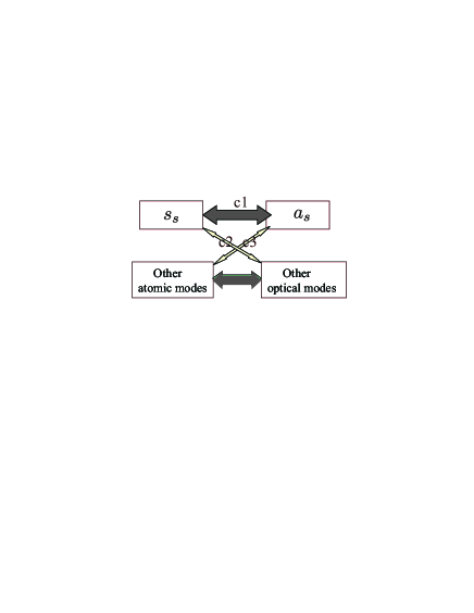
FIG. 2.: For a many-atom ensemble, The intuitive interaction picture between the atomic modes and the free-space optical modes, where c1 represents the ”good” correlation between the collective atomic mode and the signal light mode, c2 represents the spontaneous emission loss, and c3 represents the inherent mode mismatching noise. Broader connections stand for stronger correlations between the excitations in the corresponding modes.

The applications of this system for quantum information processing exactly comes from the almost pure correlation between the modes $s_{s}$ and $a_{s}$. If we neglect the weak correlations between the good modes $s_{s},a_{s}$ and the other noisy atomic and optical modes, that is, we neglect the two sources of noise illustrated in Fig. 2, all the noisy modes can be traced over, and we get effectively a two-mode problem. The excitations in the modes $s_{s}$ and $a_{s}$ can be both separately measured. For the signal mode $a_{s}$, this is done through a single-photon detector with an appropriate mode-matching; and for the atomic mode $s_{s}$, this can be done by first mapping the atomic excitation to an excitation in the signal mode through a repumping laser pulse [12], and then detecting it again through a single-photon detector. Using the almost pure correlation between the modes $s_{s}$ and $a_{s}$, one can generate some preliminarily entanglement between two distant atomic ensembles by only linear optics means, which forms the important first step for applications of this setup for different kinds of quantum information processing tasks detailed in Refs. [12, 13]. Here, we will briefly explain the basic ideas on how to entangle atomic ensembles using the correlation between the modes $s_{s}$ and $a_{s}$. This explanation helps us to define the most relevant quantities for the applications that we need to calculate.

The setup for entanglement generation between the two distant atomic ensembles L and R is shown by Fig. 3. We apply simultaneously two short Raman pumping pulses on the ensembles L and R, respectively, so that for each  ensemble the light scattered to the signal mode $a_{s}$ has a mean photon number much smaller than $1$. The signal modes are then coupled to optical channels (such as fibers) through mode matching after the filters, which are polarization and frequency selective to filter the pumping light. The signal pulses after the transmission channels interfere at a 50%-50% beam splitter BS, with the outputs detected respectively by two single-photon detectors D1 and D2. If either D1 or D2 registers one photon, the process is finished. Otherwise, we first apply a repumping laser pulse to the transition $\left|s\right\rangle\rightarrow\left|e\right\rangle$ on the ensembles L and R to set the atoms back to the ground state $\left|g\right\rangle$, then the same Raman driving pulses as the first round are applied to the transition $\left|g\right\rangle\rightarrow\left|e\right\rangle$ and we detect again the photon number of the signal modes after the beam splitter. This process is repeated until finally we have a click in either D1 or D2 detector.

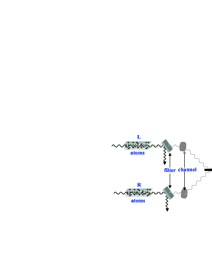
FIG. 3.: The schematic setup for generating entanglement between two distant atomic ensembles L and R.

We show now how the entanglement is generated between the ensembles L and R if we successfully register one photon in D1 or D2 detector. To understand this, let us first look at one ensemble. Before the Raman pumping pulse, the collective atomic mode $s_{s}$ and the signal light mode $a_{s}$ are in vacuum states, which are denoted respectively by $\left|0_{a}\right\rangle$, $\left|0_{p}\right\rangle$. If we neglect the small noisy correlations, after the weak pumping, the state of the the modes $s_{s}$ and $a_{s}$ has the following form (see the next section for the detailed derivation)

$$\left|\phi\right\rangle=\left|0_{a}\right\rangle\left|0_{p}\right\rangle+\sqrt{p_{c}}s_{s}^{\dagger}a_{s}^{\dagger}\left|0_{a}\right\rangle\left|0_{p}\right\rangle+o\left(p_{c}\right),$$ (3)

where $p_{c}\ll 1$ is the probability for one atom excited to the collective atomic mode $s_{s}$, and $o\left(p_{c}\right)$ represents the high-order terms with more excitations whose probabilities are equal to or smaller than $p_{c}^{2}$.

In Fig. 3, the pumping pulses excite both ensembles simultaneously, the whole system is thus described by the state $\left|\phi\right\rangle_{L}\otimes\left|\phi\right\rangle_{R}$, where $\left|\phi\right\rangle_{L}$ and $\left|\phi\right\rangle_{R}$ are given by Eq. (1) with all the operators and states distinguished by the subscript $L$ or $R$, respectively. The two signal light modes are superposed at the beam splitter, and a photodetector click in either D1 or D2 measures respectively the operators $a_{+}^{\dagger}a_{+}$ or $a_{-}^{\dagger}a_{-}$ with $a_{\pm}=\left(a_{sL}\pm e^{i\varphi}a_{sR}\right)/\sqrt{2}$. Here, $\varphi$ denotes the difference of the phase shifts in the two-side optical channels. Conditional on the detector click, we should apply a projection operator $a_{+}$ or $a_{-}$ onto the whole state $\left|\phi\right\rangle_{L}\otimes\left|\phi\right\rangle_{R}$. If we neglect the high-order corrections in Eq. (3), the projected state of the ensembles L and R thus has the form

$$\left|\Psi_{\varphi}\right\rangle_{LR}^{\pm}=\left(s_{sL}^{\dagger}\pm e^{i\varphi}s_{sR}^{\dagger}\right)/\sqrt{2}\left|0_{a}\right\rangle_{L}\left|0_{a}\right\rangle_{R},$$ (4)

which is maximally entangled in the excitation number basis. The generation of this kind of state forms the basis of further applications in quantum information processing [12, 13]. If we take into account the high-order terms in Eq. (3), the fidelity between the actually generated state and the ideal state (4) will decrease by an amount proportional to $p_{c}$, and this decrease will contribute to the final fidelity imperfection of the schemes in Refs. [12, 13]. For the applications described by these schemes, we need to fix the fidelity imperfection to be small, which means that we should keep a small excitation probability $p_{c}$ by controlling the intensity of the Raman pumping laser.

Now we look at the influence of the two types of noisy correlations illustrated in Fig. 2. The spontaneous emission loss can be quantified by the probability $p_{\text{spon}}$ of the event that the scattered photon goes to some other optical modes instead of the signal mode $a_{s}$ while the accompanying atom is excited to the collective atomic mode $s_{s}$. Without the spontaneous emission loss, for each round of Raman pumping, we succeed with a probability $2p_{c}$ to get a detector click, which prepares the entangled state (4). However, the spontaneous emission loss means that even if an atom is excited to the mode $s_{s}$ (which has a probability $p_{c}$ for each ensemble), the accompanying photon, with a probability $1-p_{\text{spon}}$, cannot be registered. For entanglement generation, the fidelity imperfection to the ideal state (4) is given by the excitation probability of the atomic mode $s_{s}$, which is now $p_{c}/\left(1-p_{\text{spon}}\right)$ instead of $p_{c}$ (we always use $p_{c}$ to denote the possibility of the good event described by Eq. (3)). To fix the fidelity imperfection to be small, in the presence of the spontaneous emission loss, we need to further decrease the excitation probability $p_{c}$ by a factor of $1-p_{\text{spon}}$, which means that we have a smaller probability to register one signal photon. So, as a result of this noise, the preparation efficiency (the success probability of the scheme) is decreased by a factor of $1-p_{\text{spon}}$ when we fix the fidelity imperfection.

The inherent mode-mismatching noise can be quantified by the probability $p_{\text{mode}}$ of the event that an atom is excited to some other atomic modes instead of the collective mode $s_{s}$ while the accompanying photon goes to the right signal mode $a_{s}$. In this case, we can register a photon from the single-photon detectors, but the atomic mode $s_{s}$ will be actually still in the initial vacuum state $\left|0_{a}\right\rangle$. So, this noise will add some vacuum component to the generated state between the ensembles L and R. In the presence of this noise, the generated state between the ensembles L and R is mixed with the form

$$\rho_{LR}\left(c_{0},\varphi\right)=\frac{1}{c_{0}+1}\left(c_{0}\left|0_{a}0_{a}\right\rangle_{LR}\left\langle 0_{a}0_{a}\right|+\left|\Psi_{\varphi}\right\rangle_{LR}^{\text{ }+}\left\langle\Psi_{\varphi}\right|\right),$$ (5)

where the vacuum coefficient $c_{0}$ is basically given by the conditional probability $p_{\text{mode}}$ for this noise contribution. Actually, as has been shown in [12], there are other sources of noise which can contribute to the vacuum coefficient $c_{0}$, such as the detector dark counts, and the detector inefficiency in the succeeding entanglement connection scheme detailed in Ref. [12]. It has also been shown there the vacuum component noise will be finally automatically purified, and thus has no influence on the final communication fidelity. However, it has a more significant influence on the efficiency than the spontaneous emission loss. For applications in Refs. [12, 13], to get a better overall efficiency, it is better to keep a balance between the mode mismatching noise $p_{\text{mode}}$ and the spontaneous emission inefficiency $p_{\text{spon}}$, with $p_{\text{mode}}$ significantly smaller than $p_{\text{spon}}$.

It is helpful to make a comparison here with the single-atom case. For a single atom interacting with the free-space light with the same level configuration as shown in Fig. 1, there is only one atomic mode given by $s=\left|g\right\rangle\left\langle s\right|$, but there are still infinite optical modes. We can still identify the forward scattered optical mode $a_{s}$ as the signal mode. The interaction picture is then shown intuitively by Fig. 4. For a single atom, there is no inherent mode-mismatching noise, but the spontaneous emission inefficiency becomes much larger. If the atom is excited to the level $\left|s\right\rangle$ (that is, to the mode $s$) through the Raman laser pumping, the accompanying photon has a probability to go to all the possible directions [16], and thus has only a very small possibility to go to the signal mode $a_{s}$. We will calculate in the following sections the spontaneous emission inefficiencies for the signal atom case as well as for the atomic ensemble case, and compare them with the different mode-matching methods to see whether there is collective enhancement of the signal-to-noise ratio for the many-atom ensemble.

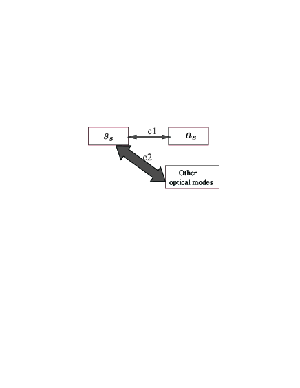
FIG. 4.: The intuitive interaction picture for the single-atom case with the corresponding symbols having the same meaning as Fig. 2. There is only one atomic mode, but the spontaneous emission loss represented by c2 becomes much larger compared with the good correlation c1.

III The theoretical model for the light-atomic-ensemble interaction and its solution

We will now go to the detailed description of the light-atomic-ensemble interaction. From this description, we will calculate the signal-light mode structure $f_{{\bf k}}$, the spontaneous emission inefficiency $p_{\text{spon}}$, and the inherent mode-mismatching noise $p_{\text{mode}}$. In the interaction configuration shown by Fig. 1, the Raman pumping laser can be described classically by neglecting its small quantum variance, and is assumed to be propagating basically along the $z$ direction. So, we can write its amplitude as $\varepsilon_{ge}\left({\bf r},t\right)=u\left({\bf r},t\right)e^{i\left(k_{0}z-\omega_{0}t\right)}$, where $\omega_{0}=k_{0}c=2\pi c/\lambda_{0}$ is the carrier frequency and $u\left({\bf r},t\right)$ is a slow varying function of the coordinate ${\bf r}$ and the time $t$. The field $\varepsilon_{se}$ coupling to the transition $|e\rangle\rightarrow|s\rangle$ should be described quantum mechanically, and we expand it into plane wave modes $\varepsilon_{se}\left({\bf r},t\right)\propto\int a_{{\bf k}}e^{i\left({\bf k\cdot r}-\omega_{{\bf k}}t\right)}d^{3}{\bf k}$ with $\omega_{{\bf k}}=\left|{\bf k}\right|c$, and $a_{{\bf k}}$, the corresponding annihilation operator. Then, the Hamiltonian describing the light-atom interaction has the following form in the interaction picture (setting $\hbar=1$)

$$H\left(t\right) = \Delta\sum_{i=1}^{N_{a}}\sigma_{ee}^{i}+\left\{g_{eg}\sum_{i=1}^{N_{a}}\sigma_{eg}^{i}u\left({\bf r}_{i},t\right)e^{ik_{0}z}\right.$$ (7)

$$\left.+\sum_{i=1}^{N_{a}}\sigma_{se}^{i}\int g_{se}^{{\bf k}}a_{{\bf k}}^{\dagger}e^{-i\left[{\bf k\cdot r}_{i}-\left(\omega_{{\bf k}}-\omega_{0}+\omega_{sg}\right)t\right]}d^{3}{\bf k+H.c.}\right\},$$

where the detuning $\Delta=\omega_{eg}-\omega_{0}$ with $\omega_{eg}=\omega_{e}-\omega_{g}$, the frequency difference between the atomic levels, $\sigma_{\mu\nu}^{i}=\left|\mu\right\rangle_{i}\left\langle\nu\right|$ ($\mu,\nu=g,e,s$) are the transition operators of the $i$th atom, ${\bf r}_{i}$ is the coordinate of the $i$th atom, and $g_{eg},g_{se}^{{\bf k}}$ are the coupling coefficients which are proportional to the dipole moments of the corresponding transitions. The coefficient $g_{se}^{{\bf k}}$ depends in general on the direction of the wave vector ${\bf k}$ by the dipole pattern. In Eq. (6), the carrier frequency of the spontaneous emission field $\varepsilon_{se}\left({\bf r},t\right)$ is given by $\omega_{0}-\omega_{sg}$, and its relevant frequency width can be estimated by the natural width $\Gamma$ of the excited level $|e\rangle$, which means that the modes $a_{{\bf k}}$ with the frequency difference between $\omega_{{\bf k}}$ and $\omega_{0}-\omega_{sg}$ much larger than the width $\Gamma$ will have negligible influence on the system dynamics. We neglect in Eq. (6) the spontaneous emission back to the level $|g\rangle$ since it is not important for our purpose (with the detection method specified in Sec. II), and has no influence on all of our results.

If both the natural width $\Gamma$ and the frequency spreading of the pumping laser $u\left({\bf r},t\right)$ are significantly smaller than the detuning $\Delta$, we can adiabatically eliminate the upper level $|e\rangle$ through the standard technique, and the resulting adiabatic Hamiltonian is given by

$$H\left(t\right) = -\left\{\sum_{i=1}^{N_{a}}\sigma_{sg}^{i}u\left({\bf r}_{i},t\right)\int\frac{g_{eg}g_{se}^{{\bf k}}}{\Delta}a_{{\bf k}}^{\dagger}e^{-i\left[\Delta{\bf k\cdot r}_{i}-\Delta\omega_{{\bf k}}t\right]}d^{3}{\bf k}\right.$$ (9)

$$\left.{\bf+H.c.}\right\}-\frac{\left|g_{eg}\right|^{2}}{\Delta}\sum_{i=1}^{N_{a}}\sigma_{gg}^{i}\left|u\left({\bf r}_{i},t\right)\right|^{2},$$

where $\Delta\omega_{{\bf k}}=\omega_{{\bf k}}-\left(\omega_{0}-\omega_{sg}\right)$ and $\Delta{\bf k=k-}k_{0}{\bf z}_{0}$ with ${\bf z}_{0}$, the unit vector in the $z$ direction. We have neglected in Eq. (7) the Stark shift of the level $|s\rangle$ since it is much smaller than the other terms (The spontaneous emission field is much weaker than the pumping field). The last term in Eq. (7) (the Stark shift of the level $|g\rangle$)can be eliminated if we make a phase rotation of the basis $\left\{|g\rangle,|s\rangle\right\}$ which will transform $\sigma_{sg}^{i}$ to $\sigma_{sg}^{i}e^{i\left(\left|g_{eg}\right|^{2}/\Delta\right)\int_{0}^{t}\left|u\left({\bf r}_{i},\tau\right)\right|^{2}d\tau}$. Thus, we can simply drop off the last term, and replace $u\left({\bf r}_{i},t\right)$ by $u^{\prime}\left({\bf r}_{i},t\right)=u\left({\bf r}_{i},t\right)e^{i\left(\left|g_{eg}\right|^{2}/\Delta\right)\int_{0}^{t}\left|u\left({\bf r}_{i},\tau\right)\right|^{2}d\tau}$. In the following, for simplicity of the symbol, we will denote $u^{\prime}\left({\bf r}_{i},t\right)$ still by $u\left({\bf r}_{i},t\right)$, and denote $-g_{eg}g_{se}^{{\bf k}}/\Delta$ by a single coefficient $g_{{\bf k}}$.

At the beginning, all the atoms and in the ground state $|g\rangle$, and all the optical modes $a_{{\bf k}}$ are in the vacuum state. We denote this initial state of all the atomic and optical modes by $|$vac$\rangle$. Then, if the Raman pumping laser $u\left({\bf r},t\right)$ is short and weak enough, we can expand the final state $|\Psi_{f}\rangle$ into a perturbative expansions. To the second order of the perturbation, the final state has the form

$$|\Psi_{f}\rangle = \left\{1-i\int_{0}^{t_{0}}H\left(\tau\right)d\tau\right.$$ (11)

$$\left.-\frac{1}{2}T\left[\int_{0}^{t_{0}}\int_{0}^{t_{0}}H\left(\tau_{1}\right)H\left(\tau_{2}\right)d\tau_{1}d\tau_{2}\right]\right\}|\text{vac}\rangle$$

where $t_{0}$ is the duration of the Raman pulse, and $T\left[\cdots\right]$ denotes the time-ordered product.

At this point, we should note that for an atomic vapor, the atom positions ${\bf r}_{i}$ are randomly distributed, and during the light-atom interaction, the atoms are moving fast in the room-temperature [17]. Therefore, we should treat ${\bf r}_{i}$ in the Hamiltonian (7) as stochastic variables. We make the following two assumptions about the properties of these variables: (i) For different atoms $i$ and $j$, ${\bf r}_{i}$ and ${\bf r}_{i}$ do not correlate with each other; (ii) Different stochastic variables ${\bf r}_{i}$ obey the same probability distribution which is determined by the geometry of the atomic cell. Note that these two assumptions are well satisfied by the room-temperature atomic gas. If the atom positions ${\bf r}_{i}$ behave as classical random variables, we should take an average of the final state $|\Psi_{f}\rangle$ over the joint probability distribution of these variables, and the resulting state becomes mixed with

$$\rho_{f}=\left\langle|\Psi_{f}\rangle\left\langle\Psi_{f}\right|\right\rangle_{\left\{{\bf r}_{i}\right\}},$$ (12)

where the symbol $\left\langle\cdots\right\rangle_{\left\{{\bf r}_{i}\right\}}$ denotes the average over all the variables ${\bf r}_{i}$.

To take the average in Eq. (9), first we note that the Hamiltonian (7) can be written as

$$H\left(t\right)=\sum_{i=1}^{N_{a}}H_{i}\left({\bf r}_{i},t\right)$$ (13)

with

$$H_{i}\left({\bf r}_{i},t\right)=\sigma_{sg}^{i}\int g_{{\bf k}}a_{{\bf k}}^{\dagger}e^{i\Delta\omega_{{\bf k}}t}\left\{u\left({\bf r}_{i},t\right)e^{-i\Delta{\bf k\cdot r}_{i}}\right\}d^{3}{\bf k.}$$ (14)

Only the term in the large bracket of the Hamiltonian $H_{i}$ depends on the variable ${\bf r}_{i}$. By the property (i) of the variables ${\bf r}_{i}$, we have

$$\left\langle H_{i}H_{j}\right\rangle_{\left\{{\bf r}_{i}\right\}} = \left\langle H_{i}\right\rangle_{\left\{{\bf r}_{i}\right\}}\left\langle H_{j}\right\rangle_{\left\{{\bf r}_{i}\right\}}$$ (16)

$$+\delta_{ij}\left\{\left\langle H_{i}^{2}\right\rangle_{\left\{{\bf r}_{i}\right\}}-\left\langle H_{i}\right\rangle_{\left\{{\bf r}_{i}\right\}}^{2}\right\}.$$

By the property (ii) of the variables ${\bf r}_{i}$, we know that $\left\langle u\left({\bf r}_{i},t\right)e^{-i\Delta{\bf k\cdot r}_{i}}\right\rangle_{\left\{{\bf r}_{i}\right\}}$ becomes independent of the atom index $i$, so the average of the Hamiltonian $H\left(t\right)$ has the simple form

$$\left\langle H\left(t\right)\right\rangle_{\left\{{\bf r}_{i}\right\}} = \sqrt{N_{a}}s_{s}$$ (18)

$$\times\int g_{{\bf k}}a_{{\bf k}}^{\dagger}e^{i\Delta\omega_{{\bf k}}t}\left\langle u\left({\bf r}_{i},t\right)e^{-i\Delta{\bf k\cdot r}_{i}}\right\rangle_{\left\{{\bf r}_{i}\right\}}d^{3}{\bf k,}$$

where $s_{s}$ is the symmetrical collective atomic operators defined in Eq. (1). We will write the initial vacuum state $|$vac$\rangle$ as a tensor product of the atomic part $|$vac$\rangle_{a}$ and the optical part $|$vac$\rangle_{p}$, and denote the atomic state $\sigma_{sg}^{i}|$vac$\rangle_{a}$ simply by $|s\rangle_{i}$. With this notation, a combination of Eqs. (8)-(13) yields the following form for the averaged state $\rho_{f}$

$$\rho_{f}=\left(1-p_{2}-p_{c}\right)|\Psi_{\text{eff}}\rangle\left\langle\Psi_{\text{eff}}\right|+p_{2}\rho_{n}+o\left(p_{2}\right),$$ (19)

where the effective pure state $|\Psi_{\text{eff}}\rangle$ (not-normalized) is

$$|\Psi_{\text{eff}}\rangle=\left(1-i\int_{0}^{t_{0}}\left\langle H\left(\tau\right)\right\rangle_{\left\{{\bf r}_{i}\right\}}d\tau\right)|vac\rangle,$$ (20)

with $\left\langle\Psi_{\text{eff}}\right|\Psi_{\text{eff}}\rangle=1+p_{c}$, and the noise component $p_{2}\rho_{n}$ is given by

$$p_{2}\rho_{n} = \sum_{i=1}^{N_{a}}|s\rangle_{i}\left\langle s\right|\otimes\int_{0}^{t_{0}}\int_{0}^{t_{0}}d\tau_{1}d\tau_{2}\int d^{3}{\bf k}\int d^{3}{\bf k}^{\prime}$$ (24)

$$\times g_{{\bf k}}g_{{\bf k}^{\prime}}^{\ast}e^{i\left(\Delta\omega_{{\bf k}}\tau_{1}-\Delta\omega_{{\bf k}^{\prime}}\tau_{2}\right)}a_{{\bf k}}^{\dagger}|\text{vac}\rangle_{p}\left\langle\text{vac}\right|a_{{\bf k}^{\prime}}$$

$$\times\left\{\left\langle u\left({\bf r}_{i},\tau_{1}\right)u^{\ast}\left({\bf r}_{i},\tau_{2}\right)e^{-i\left({\bf k-k}^{\prime}\right){\bf\cdot r}_{i}}\right\rangle_{\left\{{\bf r}_{i}\right\}}\right.$$

$$\left.-\left\langle u\left({\bf r}_{i},\tau_{1}\right)e^{-i\Delta{\bf k\cdot r}_{i}}\right\rangle_{\left\{{\bf r}_{i}\right\}}\left\langle u\left({\bf r}_{i},\tau_{2}\right)e^{i\Delta{\bf k}^{\prime}{\bf\cdot r}_{i}}\right\rangle_{\left\{{\bf r}_{i}\right\}}\right\},$$

with the value of $p_{2}$ determined by the normalization of $\rho_{n}$, i.e., by $tr\left(\rho_{n}\right)=1$. In Eq. (14), $o\left(p_{2}\right)$ represents the higher-order terms compared with the magnitude of $p_{2}$ and $p_{c}$, which will be neglected in the following. We also ignored the second-order cross-terms proportional to $\sigma_{sg}^{i}a_{{\bf k}}^{\dagger}|$vac$\rangle\left\langle\text{vac}\right|$ or $|$vac$\rangle\left\langle\text{vac}\right|\sigma_{gs}^{i}a_{{\bf k}}$ in writing Eq. (14), since they have no contributions to the quantities we will calculate in the below. The solution (14) serves as the starting point for discussions of various properties of this system in the following section.

IV Properties of the light-atomic-ensemble interaction

Now, let us analyze the properties of the light-atomic-ensemble interaction revealed by the solution (14). First, we look at the effective pure state $|\Psi_{\text{eff}}\rangle$ by neglecting the noise component $p_{2}\rho_{n}$. The state $|\Psi_{\text{eff}}\rangle$ has exactly the same form as the ideal state (3) which is the starting point for all the applications. To see this clearly, we can write $|\Psi_{\text{eff}}\rangle$ as $|\Psi_{\text{eff}}\rangle=\left(1+\sqrt{p_{c}}s_{s}^{\dagger}a_{s}^{\dagger}\right)|$vac$\rangle$, by defining the signal mode

$$a_{s}^{\dagger} \equiv \int f_{{\bf k}}a_{{\bf k}}^{\dagger}d^{3}{\bf k}$$ (25)

$${\bf\equiv} -i\frac{\sqrt{N_{a}}}{\sqrt{p_{c}}}\int d^{3}{\bf k}\int_{0}^{t_{0}}d\tau g_{{\bf k}}a_{{\bf k}}^{\dagger}e^{i\Delta\omega_{{\bf k}}\tau}\left\langle u\left({\bf r}_{i},\tau\right)e^{-i\Delta{\bf k\cdot r}_{i}}\right\rangle_{\left\{{\bf r}_{i}\right\}}{\bf,}$$ (26)

where the value of $p_{c}$ is determined by the normalization of the operator $a_{s}^{\dagger}$, i.e., by the condition $\left[a_{s},a_{s}^{\dagger}\right]=1$.

We are particularly interested in the spatial structure of the signal mode $a_{s}^{\dagger}$, since one needs to know this spatial structure to design mode-matching in practical experiments. The integration $\int d^{3}{\bf k}$ can be expressed as $\int d^{3}{\bf k=}\int_{\omega_{0}-\omega_{sg}-\delta/2}^{\omega_{0}-\omega_{sg}+\delta/2}d\omega\int_{4\pi}d\Omega$, where $d\Omega=\sin\theta d\theta d\varphi$ represents the infinitesimal solid angle and $\delta$ is the bandwidth of the spontaneous emission field which is in the order of the natural width $\Gamma$ of the excited level $|e\rangle$. The spatial structure of the mode $a_{s}^{\dagger}$ is determined by the superposition coefficient $f_{{\bf k}}=f\left(\omega,\Omega\right)$ as a function of the solid angle $\Omega$. Typically, the size $L$ of the atomic ensemble (centimeter long or less) satisfies the condition $\Gamma L/c\ll 1$, and $\omega_{sg}L/c\ll 1$ ($\omega_{eg}$ is either around GHz or zero, depending on one uses the hyperfine level or the Zeeman sublevel for the $|s\rangle$ state). In this case, $\Delta{\bf k\cdot r}_{i}=\left({\bf k-}k_{0}{\bf z}_{0}\right){\bf\cdot r}_{i}\simeq k_{0}\left({\bf k/}\left|{\bf k}\right|-{\bf z}_{0}\right){\bf\cdot r}_{i}$, which only depends on the direction of ${\bf k}$, and becomes independent of the frequency $\omega$. We assume that the Raman pumping field can be factorized as $u\left({\bf r},t\right)=u_{\perp}\left({\bf r}\right)\mu_{l}\left(z,t\right)$, where $\mu_{l}\left(z,t\right)$ is a slowly changing function of the coordinate, and can be well approximated as a constant along the size of the atomic ensemble. With this condition, the superposition function $f\left(\omega,\Omega\right)$ is factorized as a product of the frequency part $f_{\omega}\left(\omega\right)$ and the spatial part $f_{\Omega}\left(\Omega\right)$, and the spatial part $f_{\Omega}\left(\Omega\right)$ becomes independent of the emission frequency $\omega$ and the interaction time $t_{0}$. To have a more explicit expression of the spatial structure $f_{\Omega}\left(\Omega\right)$ of the signal mode $a_{s}^{\dagger}$, we assume that the atoms are distributed by the normalized distribution function $p_{\text{dis}}\left({\bf r}\right)$ (with $\int p_{\text{dis}}\left({\bf r}\right)d^{3}{\bf r}=1$), which is determined by the geometry of the ensemble. As we mentioned before, the interaction coefficient $g_{{\bf k}}$ normally also depends on the direction of the wave vector ${\bf k}$ in the form of a dipole pattern, but it varies very slowly with the angle $\Omega$ compared with other contributions in $f_{\Omega}\left(\Omega\right)$, so we drop it off when considering the spatial structure of the signal mode. Under this circumstance, $f_{\Omega}\left(\Omega\right)$ is simply expressed as

$$f_{\Omega}\left(\Omega\right) = \left\langle u_{\perp}\left({\bf r}\right)e^{-i\Delta{\bf k\cdot r}_{i}}\right\rangle_{\left\{{\bf r}_{i}\right\}}$$ (27)

$$= \int d^{3}{\bf r}u_{\perp}\left({\bf r}\right)p_{\text{dis}}\left({\bf r}\right)e^{ik_{0}z\left(1-\cos\theta\right)-ik_{0}\sin\theta\left(x\cos\varphi+y\sin\varphi\right)}.$$ (28)

To further simplify this expression, we assume a Gaussian pump beam with $u_{\perp}\left({\bf r}\right)=e^{-\left(x^{2}+y^{2}\right)/r_{0}^{2}}$, and a Gaussian form for the transverse part of the atomic distribution function with [18]

$$p_{\text{dis}}\left({\bf r}\right) = \frac{1}{\pi LR_{0}^{2}}e^{-\left(x^{2}+y^{2}\right)/R_{0}^{2}},\text{ (}-L/2\leq z\leq L/2),$$ (29)

$$p_{\text{dis}}\left({\bf r}\right) = 0,\text{ \ \ \ \ \ \ \ \ \ \ \ \ \ }\left(z<-L/2,\text{ or, }z>L/2\right)$$ (30)

where $r_{0}$ and $R_{0}$ characterize the radius of the pump beam and the radius of the atomic ensemble, respectively, and $L$ is the length of the ensemble. In this case, we have an analytic expression for the signal mode function

$$f_{\Omega}\left(\Omega\right)=\frac{r_{0}^{2}}{r_{0}^{2}+R_{0}^{2}}e^{-\frac{1}{4}k_{0}^{2}r_{0}^{2}R_{0}^{2}\sin^{2}\theta/\left(r_{0}^{2}+R_{0}^{2}\right)}\mathop{\rm sinc}\left(k_{0}L\sin^{2}\frac{\theta}{2}\right),$$ (31)

where the function $\mathop{\rm sinc}$ is defined as $\mathop{\rm sinc}\left(x\right)\equiv\sin\left(x\right)/x$. From this expression, we see that the signal photon mainly goes to the forward direction. The signal mode is inside a small cone around $\theta=0$ with $\Delta\theta$ characterized by $\min\left[\sqrt{r_{0}^{2}+R_{0}^{2}}/\left(k_{0}r_{0}R_{0}\right),1/\sqrt{k_{0}L}\right]$.

We have shown that the first component of the solution (14) exactly contributes to the ideal coherent process, and have specified the spatial structure of the signal mode. Now we analyze the contributions of the noise described by the second component of Eq. (14). From Eq. (14), we see that the noise component $p_{2}\rho_{n}$ is expressed as a tensor product of the atomic density operator $\rho_{n}^{a}=\sum_{i=1}^{N_{a}}|s\rangle_{i}\left\langle s\right|$ and the remaining optical density operator $\rho_{n}^{p}$. Besides the symmetric collective atomic mode $s_{s}$ and the signal optical mode $a_{s}$, there are many other noise modes contributing to the atomic density operator $\rho_{n}^{a}$ and the optical density operator $\rho_{n}^{p}$. These noise modes correlate with each other in a complicated way, however, these correlations do not contribute to the noise of the relevant dynamics if the two signal modes are not involved in the correlations, since the reduced density operator of the modes $s_{s}$ and $a_{s}$, which describes the relevant dynamics, will not be influenced by these correlations after we take trace over all the noise modes. Nevertheless, the correlations between the good modes and the noisy mode will have influence on the relevant dynamics, and these contribute to the two sources of noise we have mentioned before: the spontaneous emission loss and the inherent mode-matching inefficiency. These two sources of noise are described quantitatively by the conditional probabilities $p_{\text{spon}}$ and $p_{\text{mode}}$, respectively. The $p_{\text{spon}}$ represents the probability that an atom is excited to the right mode $s_{s}$, but the accompanying photon does not go to the signal mode $a_{s}$. From the solution (14) to the whole density operator $\rho_{f}$, this possibility can be expressed as

$$p_{\text{spon}}=1-\frac{tr\left(\left\langle 0_{a}0_{p}\right|a_{s}s_{s}\rho_{f}s_{s}^{\dagger}a_{s}^{\dagger}|0_{a}0_{p}\rangle\right)}{tr\left(\left\langle 0_{a}\right|s_{s}\rho_{f}s_{s}^{\dagger}|0_{a}\rangle\right)},$$ (32)

where $tr\left(\cdots\right)$ represents the trace over all the remaining atomic and optical modes involved in the operator $\rho_{f}$. Similarly, $p_{\text{mode}}$ represents the probability that a photon is emitted to the signal mode $a_{s}$, but the accompanying atomic excitation is not in the right mode $s_{s}$, and this possibility can be expressed from the density operator $\rho_{f}$ as

$$p_{\text{mode}}=1-\frac{tr\left(\left\langle 0_{a}0_{p}\right|a_{s}s_{s}\rho_{f}s_{s}^{\dagger}a_{s}^{\dagger}|0_{a}0_{p}\rangle\right)}{tr\left(\left\langle 0_{p}\right|a_{s}\rho_{f}a_{s}^{\dagger}|0_{p}\rangle\right)}.$$ (33)

In the following, we need to calculate these two probabilities to quantify the noise magnitudes.

From the solution (14), we can derive the probability $tr\left(\left\langle 0_{a}\right|s_{s}\rho_{f}s_{s}^{\dagger}|0_{a}\rangle\right)$ for one atomic excitation in the mode $s_{s}$, the possibility $tr\left(\left\langle 0_{p}\right|a_{s}\rho_{f}a_{s}^{\dagger}|0_{p}\rangle\right)$ for one photon in the mode $a_{s}$, and the joint possibility $tr\left(\left\langle 0_{a}0_{p}\right|a_{s}s_{s}\rho_{f}s_{s}^{\dagger}a_{s}^{\dagger}|0_{a}0_{p}\rangle\right)$ for one atom in the mode $s_{s}$ and one photon in the mode $a_{s}$. They are respectively given by

$$tr\left(\left\langle 0_{a}\right|s_{s}\rho_{f}s_{s}^{\dagger}|0_{a}\rangle\right)=p_{c}+p_{2}/N_{a},$$ (34)

$$tr\left(\left\langle 0_{p}\right|a_{s}\rho_{f}a_{s}^{\dagger}|0_{p}\rangle\right)=p_{c}+\chi p_{c},$$ (35)

$$tr\left(\left\langle 0_{a}0_{p}\right|a_{s}s_{s}\rho_{f}s_{s}^{\dagger}a_{s}^{\dagger}|0_{a}0_{p}\rangle\right)=p_{c}+\chi p_{c}/N_{a},$$ (36)

where $p_{2}$ and $p_{c}$ are obtained respectively from the normalization of $\rho_{n}$ and $a_{s}^{\dagger}$ ( see Eq. (16) and Eq. (17)), and the ratio $\chi$ is defined as

$$\chi=N_{a}tr\left(\left\langle 0_{p}\right|a_{s}\rho_{n}^{p}a_{s}^{\dagger}|0_{p}\rangle\right)/p_{c},$$ (37)

with $\rho_{n}^{p}$, the optical part of the noise component $p_{2}\rho_{n}$ as we have specified before.

From the above equations, we see that we only need to calculate the two ratios $p_{c}/p_{2}$ and $\chi$ to determine the noise probabilities $p_{\text{spon}}$ and $p_{\text{mode}}$. As we have mentioned before, the shape $u\left({\bf r},t\right)$ of the pump beam is typically decomposed as $u\left({\bf r},t\right)=u_{\perp}\left({\bf r}\right)\mu_{l}\left(z,t\right)$ with $\mu_{l}\left(z,t\right)$ approximately independent of $z$ along the size of the atomic ensemble. In this case, the two ratios $p_{c}/p_{2}$ and $\chi$ have much simplified expressions, which, become independent of the interaction details, such as the interaction time or the bandwidth of the coupling field, and depend only on some spatial integrations determined by the geometry of the atomic ensemble and the pump beam. For simplicity, we also neglect the slow variation of the coupling coefficient $g_{{\bf k}}$ with the direction of ${\bf k}$. Under these conditions, the ratios $p_{c}/p_{2}$ and $\chi$ are given respectively by

$$\frac{p_{c}}{p_{2}}=\frac{\int_{4\pi}d\Omega\left\{\left|\left\langle u_{\perp}\left({\bf r}_{i}\right)e^{-i\Delta{\bf k\cdot r}_{i}}\right\rangle_{\left\{{\bf r}_{i}\right\}}\right|^{2}\right\}}{\int_{4\pi}d\Omega\left\{\left\langle\left|u_{\perp}\left({\bf r}_{i}\right)\right|^{2}\right\rangle_{\left\{{\bf r}_{i}\right\}}-\left|\left\langle u_{\perp}\left({\bf r}_{i}\right)e^{-i\Delta{\bf k\cdot r}_{i}}\right\rangle_{\left\{{\bf r}_{i}\right\}}\right|^{2}\right\}},$$ (38)

$$\chi = \left[\int_{4\pi}d\Omega\left\{\left|\left\langle u_{\perp}\left({\bf r}_{i}\right)e^{-i\Delta{\bf k\cdot r}_{i}}\right\rangle_{\left\{{\bf r}_{i}\right\}}\right|^{2}\right\}\right]^{-2}$$ (41)

$$\times\int_{4\pi}d\Omega\int_{4\pi}d\Omega^{\prime}\left\{\left\langle\left|u_{\perp}\left({\bf r}_{i}\right)\right|^{2}e^{-i\left({\bf k-k}^{\prime}\right){\bf\cdot r}_{i}}\right\rangle_{\left\{{\bf r}_{i}\right\}}\right.$$

$$\times\left.\left\langle u_{\perp}^{\ast}\left({\bf r}_{i}\right)e^{i\Delta{\bf k\cdot r}_{i}}\right\rangle_{\left\{{\bf r}_{i}\right\}}\left\langle u_{\perp}\left({\bf r}_{i}\right)e^{-i\Delta{\bf k}^{\prime}{\bf\cdot r}_{i}}\right\rangle_{\left\{{\bf r}_{i}\right\}}\right\}-1.$$

Similar to the case for calculating the signal mode structure $f_{\Omega}\left(\Omega\right)$, we also assume a Gaussian pump beam and a Gaussian form for the transverse atomic distribution function as is shown by Eq. (19). In this case, we have the following analytic expressions for these two ratios

$$\frac{p_{c}}{p_{2}} \simeq \frac{r_{0}^{2}\left(r_{0}^{2}+2R_{0}^{2}\right)}{2\left(r_{0}^{2}+R_{0}^{2}\right)^{2}}\int_{0}^{\pi}\sin\theta d\theta\left\{e^{-\frac{1}{2}k_{0}^{2}r_{0}^{2}R_{0}^{2}\sin^{2}\theta/\left(r_{0}^{2}+R_{0}^{2}\right)}\right.$$ (43)

$$\left.\times\mathop{\rm sinc}^{2}\left(k_{0}L\sin^{2}\frac{\theta}{2}\right)\right\},$$

$$\chi = \frac{\left(r_{0}^{2}+R_{0}^{2}\right)^{2}}{r_{0}^{2}\left(r_{0}^{2}+2R_{0}^{2}\right)}\left[\int_{0}^{\pi}\sin\theta d\theta\left\{e^{-\frac{1}{2}k_{0}^{2}r_{0}^{2}R_{0}^{2}\sin^{2}\theta/\left(r_{0}^{2}+R_{0}^{2}\right)}\mathop{\rm sinc}^{2}\left(k_{0}L\sin^{2}\frac{\theta}{2}\right)\right\}\right]^{-2}$$ (46)

$$\times\int_{0}^{\pi}\int_{0}^{\pi}\sin\theta\sin\theta^{\prime}d\theta d\theta^{\prime}\left\{\frac{1}{2\pi}\int_{0}^{2\pi}e^{-\frac{1}{4}k_{0}^{2}r_{0}^{2}R_{0}^{2}\left(\sin^{2}\theta+\sin^{2}\theta^{\prime}-2\sin\theta\sin\theta^{\prime}\cos\varphi\right)/\left(r_{0}^{2}+2R_{0}^{2}\right)}d\varphi\right.$$

$$\left.\times e^{-\frac{1}{4}k_{0}^{2}r_{0}^{2}R_{0}^{2}\left(\sin^{2}\theta+\sin^{2}\theta^{\prime}\right)\left(r_{0}^{2}+R_{0}^{2}\right)}\mathop{\rm sinc}\left[k_{0}L\left(\sin^{2}\frac{\theta}{2}-\sin^{2}\frac{\theta}{2}\right)\right]\mathop{\rm sinc}\left(k_{0}L\sin^{2}\frac{\theta}{2}\right)\mathop{\rm sinc}\left(k_{0}L\sin^{2}\frac{\theta^{\prime}}{2}\right)\right\}-1.$$

In writing Eq. (29), we have assumed $k_{0}L\gg 1$ and have neglected the term which is about $1/k_{0}L$ times smaller.

From the two ratios $p_{c}/p_{2}$ and $\chi$, the spontaneous emission loss and the inherent mode matching inefficiency are directly written as

$$p_{\text{spon}}\simeq\left(1+N_{a}p_{c}/p_{2}\right)^{-1},$$ (47)

$$p_{\text{mode}}\simeq\chi/\left(1+\chi\right).$$ (48)

The approximations in Eqs. (31) and (32) are valid under the condition $N_{a}\gg 1$ (we neglected the terms which are $1/N_{a}$ times smaller). To minimize the two sources of noise $p_{\text{spon}}$ and $p_{\text{mode}}$, it is better to have a large $N_{a}p_{c}/p_{2}$ and a small $\chi$. We will discuss the details in the following section on how to minimize these two noise by using different kinds of mode matching methods.

At the end of this section, we would like to make a brief comparison with the single atom case. For the case of a single atom, if the position of this atom is also fluctuating in the space, the above calculation is still valid but with $N_{a}=1$. From Eqs. (21)-(26), we see that in the case of $N_{a}=1$, we always have $p_{\text{mode}}=0$. Thus, for the case of a single atom, the spontaneous emission loss is the only source of noise, as has been shown intuitively in Fig. 4. However, in this case, the spontaneous emission inefficiency $p_{\text{spon}}$, which can be approximated by $p_{\text{spon}}\simeq 1-\left(1+\chi\right)p_{c}/p_{2}$ since $p_{c}\ll p_{2}$, becomes much larger. If we compare the efficiency (defined as $1-p_{\text{spon}}$) from the spontaneous emission noise between the single-atom case and the atomic-ensemble case, we see that this efficiency is increased by about a factor of $N_{a}$ for the atomic ensemble. This is what we called the collective enhancement of the signal-to-noise ratio for the many-atom ensemble.

V Mode matching methods

The first mode-matching method is to choose the signal mode as the mode for detection, with the mode function exactly given by the inherent spatial structure (20) of the signal light. The mode function (20) is similar to a Gaussian function, especially when $k_{0}r_{0}^{2}>L$ and $k_{0}R_{0}^{2}>L$. (It would be an exact Gaussian function if the axial distribution of $p_{\text{dis}}\left({\bf r}\right)$ is Gaussian). One can couple a Gaussian mode into a single-mode optical fibre with a good technical mode-matching efficiency. For this case with an exact mode matching, the two noise probabilities $p_{\text{spon}}$ and $p_{\text{mode}}$ are exactly given by Eqs. (29)-(32). We now go to the calculations of these two noise probabilities. For this purpose, we need to understand first how to get a large $N_{a}p_{c}/p_{2}$ and a small $\chi$ to minimize the noise $p_{\text{spon}}$ and $p_{\text{mode}}$.

First, we give an estimation of the ratio $N_{a}p_{c}/p_{2}$. It has a definite physical meaning. From Eq. (29), we see that the integration function is significantly different to zero only when the integration variable $\theta$ falls into a small cone with $0\leq\theta<\theta_{f}$, where $\theta_{f}$ is estimated by $\theta_{f}\sim\min\left(1/\sqrt{k_{0}L},1/k_{0}r_{eff}\right)$ with $r_{eff}\equiv r_{0}R_{0}/\sqrt{r_{0}^{2}+R_{0}^{2}}$. Thus, the result of the integration can be estimated by $\theta_{f}^{2}$. We also know that the total atom number can be approximated by $N_{a}\sim n_{a}\pi R_{0}^{2}L$, where $n_{a}$ denotes the average atom number density. From this, we see that the ratio $N_{a}p_{c}/p_{2}$ is estimated by

$$\frac{N_{a}p_{c}}{p_{2}}\sim\min\left(\frac{1}{2}n_{a}\lambda_{0}r_{eff}^{2},\text{ }\frac{1}{4\pi}n_{a}\lambda_{0}^{2}L\right).$$ (49)

If we assume that the two bounds for $N_{a}p_{c}/p_{2}$ are comparable, which means that $1/\sqrt{k_{0}L}\sim 1/k_{0}r_{eff}$, or the Fresnel number defined as $Fr\equiv\pi r_{eff}^{2}/\lambda_{0}L$ is in the order of $1$, we have $N_{a}p_{c}/p_{2}\sim n_{a}\lambda_{0}^{2}L/\left(4\pi\right)\sim d_{o}/\left(4\pi\right)$, where the on-resonance optical depth $d_{o}$ is simply defined as $d_{o}\equiv n_{a}\lambda_{0}^{2}L$. Therefore, to have a small spontaneous emission inefficiency $p_{\text{spon}}$, we need to use an optically dense ensemble with $d_{o}\gg 1$ (the off-resonance optical depth can still be much smaller than $1$ due to the large detuning).

Next, we consider how to minimize the ratio $\chi$ by choosing appropriate interaction configurations. From Eq. (30), we see that $\chi$ increase with the ratio $R_{0}/r_{0}$. This can be intuitively understood as follows: the noise characterized by $p_{\text{mode}}$ and $\chi$ comes from the density fluctuation of the atomic ensemble. With a larger $R_{0}$, the atoms have more space to move around, and one thus has a relatively larger density function and a larger noise ratio $\chi$ [19]. Thus, to minimize $\chi$, we choose a configuration with $r_{0}\gg R_{0}$ in the following, which means, the pumping laser is shined on all the atoms with a broad cross section. In this case, the effective radius $r_{eff}\simeq R_{0}$.

Now we would like to calculate the noise probabilities $p_{\text{spon}}$ and $p_{\text{mode}}$ in a more accurate way in the case of exact mode matching. This requires us to carry out the complicate integrations in Eqs. (29) and (30), which is only possible by using numerical methods. The spontaneous emission inefficiency $p_{\text{spon}}$ depends on the optical depth $d_{o}=n_{a}\lambda_{0}^{2}L$. We have numerically calculated the value of $p_{\text{spon}}$ versus the optical depth $d_{o}$ under different geometries of the atomic ensemble. The geometry of the ensemble is described by the Fresnel number $Fr\equiv\pi R_{0}^{2}/\lambda_{0}L$. The calculation result is shown in Fig. 5. From the figure, we see that the spontaneous emission inefficiency is insensitive to the geometry of the ensemble. The two curves with $Fr=1$ and $Fr=10$ basically overlaps. With a much smaller $Fr=0.1$, the inefficiency $p_{\text{spon}}$ increases by about a factor of $2$. On the other hand, $p_{\text{spon}}$ is sensitive to the optical depth $d_{o}$. It decrease with $1/d_{o}$ approximately linearly, which confirms the rough estimation from the above. From the curves, we can write $p_{\text{spon}}$ approximately as $p_{\text{spon}}=1/(1+d_{o}/26)$ for the Fresnel number $F_{r}$ from $1$ to $10$. In the above numerical calculation, we assumed some typical values for the parameters with $\lambda_{0}\sim 0.8\mu$m and $L\sim 1$cm, but actually the result is very insensitive to the parameter $k_{0}L$ as long as it is still much larger than $1$. For an atomic cell with a typical number density $n_{a}\sim 10^{12}/$cm³ and length $L\sim 1$cm, the optical depth $d_{o}\sim 6.4\times 10^{3}$, and we have a spontaneous emission inefficiency $p_{\text{spon}}\sim 0.4\%$, which is very small.

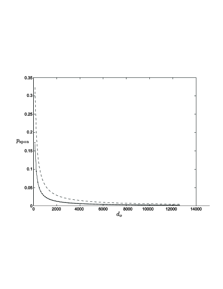
FIG. 5.: The spontaneous emission inefficiency $p_{\text{spon}}$ versus the on-resonance optical depth $d_{o}$ of the ensemble under different geometries characterized by the Fresnel number $Fr$. We have $Fr=10$ for the solid curve, $Fr=1$ for the dotted curve, and $Fr=0.1$ for the dashed curve.

The inherent mode matching inefficiency $p_{\text{mode}}$ is determined by the geometry of the ensemble, and does not depend on the value of the optical depth. We have numerically calculated the value of $p_{\text{mode}}$. It turns out that $p_{\text{mode}}$ is actually also insensitive to the geometric parameters $k_{0}L$ and $Fr$ as long as they are still in the typical region. For instance, we have $p_{\text{mode}}\simeq 24\%$ for $Fr=1$, $p_{\text{mode}}\simeq 25\%$ for $Fr=10$, and $p_{\text{mode}}\simeq 23\%$ for $Fr=0.1$. In each case, we change the length $L$ from $0.3$cm to $3$cm (with $\lambda_{0}\sim 0.8\mu$m), and the value of $p_{\text{mode}}$ basically does not change at all. Note that the typical inherent mode matching inefficiency $p_{\text{mode}}\simeq 24\%$ is quite large, and we can not efficiently reduce it by controlling the geometry of the ensemble. As we have mentioned before, the mode mismatching noise has a more significant influence on the efficiency of the application schemes than the spontaneous emission noise. The large inherent mode matching inefficiency is a disadvantage of the exact mode-matching method.

To reduce the inefficiency $p_{\text{mode}}$, we consider the following simple improvement to the exact mode matching method. After the light-atomic-ensemble interaction, the scattered light is focused by a lens, and we apply an aperture on the focal plane of the lens to collect the signal light only from a small cone in the forward direction with $0\leq\theta\leq\theta_{D}$, where the detection angle $\theta_{D}$ can be controlled by the size of the aperture. We call this kind of mode matching the filtered exact mode matching. By the exact mode matching, we detect the photon scattered to the signal mode; and by the filtered exact mode matching, we only detect the scattered photon which is in the signal mode and at the same time lies in the filtering cone with $0\leq\theta\leq\theta_{D}$. Due to the additional restriction, we now have a less success probability to register the photon. The spontaneous emission inefficiency $p_{\text{spon}}$ should increase, but through this scarification, we can significantly reduce the noise $p_{\text{mode}}$, which means, if we register the photon with this additional restriction, we are more confident that the accompanying atomic excitation will go to the collective atomic mode $s_{s}$. To calculate $p_{\text{spon}}$ and $p_{\text{mode}}$ for the filtered exact mode matching, we can still use Eqs. (21)-(26), but the signal mode $a_{s}$ should be confined inside the small cone with $0\leq\theta\leq\theta_{D}$. Inside this filtering cone, the signal mode has the same mode structure as given by Eq. (20). With this modified signal mode, we find that $p_{\text{mode}}$ is still given by Eqs. (32) and (30), but all the integrations of $\theta$ and $\theta^{\prime}$ in Eq. (30) can only be taken from $0$ to the filtering angle $\theta_{D}$ instead of from $0$ to $\pi$. The spontaneous emission inefficiency $p_{\text{spon}}$ now has the following expression

$$p_{\text{spon}}\simeq 1-\frac{N_{a}p_{c}|_{\theta\leq\theta_{D}}}{N_{a}p_{c}+p_{2}},$$ (50)

where we have assumed $N_{a}\gg 1$ for the approximation, and the symbol $p_{c}|_{\theta\leq\theta_{D}}$ means that the integration of $\theta$ in $p_{c}$ can only be taken from $0$ to $\theta_{D}$. From Eq. (34), we need to calculate two ratios $p_{c}/p_{2}$ and $p_{c}|_{\theta\leq\theta_{D}}/p_{2}$ for $p_{\text{spon}}$. The ratio $p_{c}/p_{2}$ is exactly given by Eq. (29), and the ratio $p_{c}|_{\theta\leq\theta_{D}}/p_{2}$ has the same form as Eq. (29), but the integration of $\theta$ is only from $0$ to $\theta_{D}$.

We have numerically calculate the noise probabilities $p_{\text{spon}}$ and $p_{\text{mode}}$ versus the filtering angle $\theta_{D}$, and the result is shown in Fig. 6 with the Fresnel number $Fr=1$ and the optical depth $d_{o}\sim 1.9\times 10^{3}$. From the figure, we see that by decreasing the filtering angle $\theta_{D}$, we can significantly reduce the noise $p_{\text{mode}}$. The cost is that at the same time the inefficiency $p_{\text{spon}}$ significantly increases. However, as we have mentioned before, though both of the noise $p_{\text{spon}}$ and $p_{\text{mode}}$ are correctable in the application schemes in Refs. [12, 13], the mode mismatching noise $p_{\text{mode}}$ has a more severe influence on the final efficiency of the schemes than the spontaneous emission noise $p_{\text{spon}}$. Thus, for these applications, it is worthy to choose an appropriate filtering angle $\theta_{D}$ with $p_{\text{mode}}$ significantly smaller than $p_{\text{spon}}$. For instance, if we choose the angle $\theta_{D}\simeq 0.002$, the mode mismatching noise $p_{\text{mode}}\simeq 0.9\%$, which is basically negligible compared with other sources of noise. At the same time, $p_{\text{spon}}\simeq 66.6\%$, which seems to be quite large. However, to overcome this noise, we need only to increase the repetitions of the entanglement generation scheme in Refs. [12, 13] by another factor of $3$ (given by $1/\left(1-p_{\text{spon}}\right)$), which is actually only a moderate cost. This choice would be much better than the case without any filtering, where we have an inherent mode mismatching noise $p_{\text{mode}}\simeq 24\%$. For the purpose of guiding the choice of the best experimental configuration, we list several important values of $p_{\text{spon}}$ and $p_{\text{mode}}$ versus the angle $\theta_{D}$ in the following table

$\theta_{D}$	$0.0015$	$0.0020$	$0.0025$	$0.0040$	$0.0055$
$p_{\text{mode}}$	$0.31\%$	$0.92\%$	$2.05\%$	$8.98\%$	$17.5\%$
$p_{\text{spon}}$	$79.6\%$	$66.6\%$	$52.9\%$	$19.5\%$	$5.02\%$

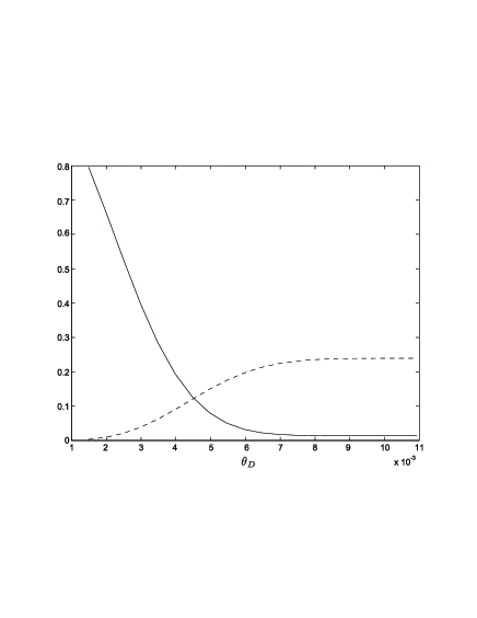
FIG. 6.: The spontaneous emission inefficiency $p_{\text{spon}}$ (solid curve) and the inherent mode mismatching probability $p_{\text{mode}}$ (dashed curve) versus the filtering angle $\theta_{D}$ with the Fresnel number $Fr=1$.

We have also calculated the noise probabilities $p_{\text{spon}}$ and $p_{\text{mode}}$ versus the angle $\theta_{D}$ under different geometries of the ensemble characterized by the Fresnel number $Fr$. For $Fr=10$ and $Fr=0.1$, the results are shown in Fig. 7. In all the calculations, we assumed the same optical depth $d_{o}\sim 1.9\times 10^{3}$ and the cell length $L\sim 1$cm. The qualitative properties of the curves for different Fresnel numbers are quite similar, but one needs to shift the appropriate angle $\theta_{D}$. With a large Fresnel number $Fr$, one needs to choose a smaller angle $\theta_{D}$. The appropriate filtering angle $\theta_{D}$ changes by a factor of $2$-$3$ if the Fresnel number changes by a factor of $10$.

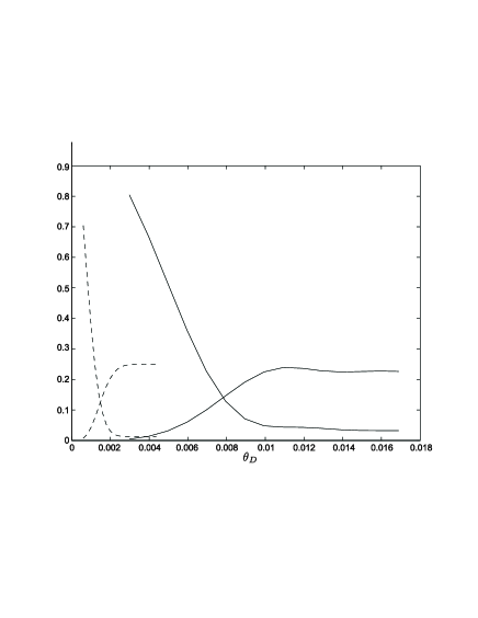
FIG. 7.: The spontaneous emission inefficiency $p_{\text{spon}}$ and the inherent mode mismatching probability $p_{\text{mode}}$ versus the filtering angle $\theta_{D}$ with the Fresnel number $Fr=10$ (the two dashed curves) and $Fr=0.1$ (the two solid curves). The spontaneous emission inefficiency increases with the decrease of the angle $\theta_{D}$ while the mode mismatching noise decreases.

Finally, we describe a mode matching method which is simplest for implementation. For this method, we still use an aperture to select the scattered light from the small cone with $0\leq\theta\leq\theta_{D}$. But now we do not use any technical mode matching to choose only the signal mode with the right mode structure $f_{\Omega}\left(\Omega\right)$ for detection. Instead, we detect the photon in all the modes which lie in the small cone with $0\leq\theta\leq\theta_{D}$. We call this the simple filtering method. This seems to be a bad mode-matching method, since one does not make any distinction between the modes in this small cone. If the registered photon does not come from the right mode $a_{s}$, the accompanying atomic excitation will be most probably not in the collective mode $s_{s}$, and one thus has a significantly larger inherent mode mismatching noise $p_{\text{mode}}$. However, the observation here is that if $\theta_{D}$ is sufficiently small, basically only the signal mode exists in this small cone, and all the other modes make negligible contributions. The important question is how small the angle $\theta_{D}$ should be to guarantee a small $p_{\text{mode}}$. Note that for the simple filtering method, the spontaneous emission inefficiency $p_{\text{spon}}$ can be calculated in the same way as the filtered exact mode matching method by the use of Eq. (34). But we have a different expression for $p_{\text{mode}}$, which in this case is defined as the probability that the accompanying atomic excitation does not go to the collective mode $s_{s}$ when one photon (from any optical modes) is detected in the small cone with $0\leq\theta\leq\theta_{D}$. This possibility can be expressed as

$$p_{\text{mode}}\simeq 1-\frac{p_{c}|_{\theta\leq\theta_{D}}+\left(1/N_{a}\right)tr\left(p_{2}\rho_{n}\right)|_{\theta\leq\theta_{D}}}{p_{c}|_{\theta\leq\theta_{D}}+tr\left(p_{2}\rho_{n}\right)|_{\theta\leq\theta_{D}}},$$ (51)

where the trace $tr\left(\cdots\right)$ is over all the atomic and the optical modes, and the symbol $|_{\theta\leq\theta_{D}}$ has the same meaning that the integrations of $\theta$ in $p_{c}$ and $tr\left(p_{2}\rho_{n}\right)$ are only from $0$ to $\theta_{D}$. In the limit of $N_{a}\gg 1$, $p_{\text{mode}}$ can still be written into the form $p_{\text{mode}}\simeq\chi_{s}/\left(1+\chi_{s}\right)$, with

$$\frac{1}{\chi_{s}+1} = \frac{p_{c}|_{\theta\leq\theta_{D}}}{tr\left(p_{2}\rho_{n}\right)|_{\theta\leq\theta_{D}}+p_{c}|_{\theta\leq\theta_{D}}}$$ (52)

$$= \frac{1}{\left(1-\cos\theta_{D}\right)}\int_{0}^{\theta_{D}}\sin\theta d\theta\left\{e^{-\frac{1}{2}k_{0}^{2}R_{0}^{2}\sin^{2}\theta}\right.$$ (54)

$$\left.\times\mathop{\rm sinc}^{2}\left(k_{0}L\sin^{2}\frac{\theta}{2}\right)\right\}.$$

In writing Eq. (36), we have assumed the same kind of atomic distribution function $p_{\text{dis}}\left({\bf r}\right)$ and the pump mode function $u_{\perp}\left({\bf r}\right)$ as we have specified before. We can use Eqs. (36) to numerically calculate the mode mismatching probability $p_{\text{mode}}$ versus the filtering angle $\theta_{D}$ for the simple filtering method. The result, together with the curve for $p_{\text{spon}}$ versus $\theta_{D}$, is shown in Fig. 8 for the Fresnel number $Fr=1$. In the calculation, we assumed the same optical depth $d_{o}\sim 1.9\times 10^{3}$. From the figure, we see that if $\theta_{D}$ is large, the mode mismatching probability $p_{\text{mode}}$ is very large, but as $\theta_{D}$ decreases, $p_{\text{mode}}$ can still tend to zero. This confirms our intuitive observation. With the same parameters, for the simple filtering method, we should further decrease the filtering angle $\theta_{D}$ by a factor of $2$-$3$ to get the optimal configuration compared with the filtered exact mode matching method. Of course, due to the decrease of the optimal $\theta_{D}$, the corresponding spontaneous emission inefficiency $p_{\text{spon}}$ significantly increases. To guide the experimental choice of the optimal $\theta_{D}$, we also list some important values of $p_{\text{spon}}$ and $p_{\text{mode}}$ for the simple filtering method

$\theta_{D}$	$0.0006$	$0.0010$	$0.0014$	$0.0020$	$0.0032$
$p_{\text{mode}}$	$1.76\%$	$4.78\%$	$9.10\%$	$17.5\%$	$37.4\%$
$p_{\text{spon}}$	$96.4\%$	$90.3\%$	$82.0\%$	$66.6\%$	$35.1\%$

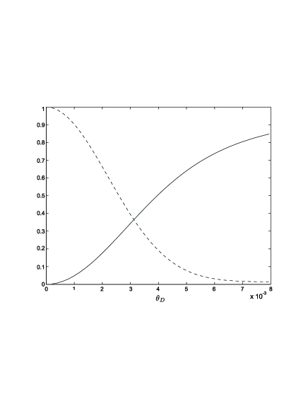
FIG. 8.: The spontaneous emission inefficiency $p_{\text{spon}}$ (dashed curve) and the inherent mode mismatching probability $p_{\text{mode}}$ (solid curve) versus the filtering angle $\theta_{D}$ with the Fresnel number $Fr=1$ for the simple filtering method.

For the simple filtering method, we also calculated the noise probabilities $p_{\text{spon}}$ and $p_{\text{mode}}$ under different geometries of the ensemble. For the Fresnel number $Fr=10$ and $Fr=0.1$, the results are shown in Fig. 9. We assumed the same optical depth and the cell length in these calculations. Since the qualitative picture revealed by this figure is quite similar to the case of the filtered exact mode matching, we do not need to discuss its properties in details.

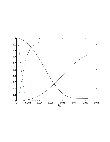
FIG. 9.: The spontaneous emission inefficiency $p_{\text{spon}}$ and the inherent mode mismatching probability $p_{\text{mode}}$ versus the filtering angle $\theta_{D}$ with the Fresnel number $Fr=10$ (the two dashed curves) and $Fr=0.1$ (the two solid curves) for the simple filtering method.

For experimental realizations, the simple filtering method can be much easier than other mode matching methods. The calculation here shows that the price we need to pay for this simplification is to choose a smaller filtering angle with a significantly increased spontaneous emission inefficiency. Note that for the application schemes in Refs. [12, 13], this price seems to be still acceptable. For instance, if we choose $\theta_{D}\simeq 0.001$, the mode mismatching noise $p_{\text{mode}}\simeq 4.8\%$ has already been small. In this case, the additional repetitions of the entanglement generation scheme in Refs. [12, 13] is given by the factor $1/\left(1-p_{\text{spon}}\right)\simeq 10$, which is not too much.

VI Summary

In summary, we have developed a theory in the weak pumping limit to describe the three-dimensional effects in the interaction between the free-space light and the many-atom ensemble. The calculations demonstrate some interesting results which are not know from the other approaches: firstly, it shows that the signal light has an inherent spatial mode structure, which is determined together by the geometry of the ensemble and the mode structure of the pump beam. Secondly, it reveals that there will be two sources of noise during the light-atom interaction. One is the spontaneous emission inefficiency, which is inversely proportional to the on-resonance optical depth of the ensemble; and the other is the inherent mode mismatching noise, which arises from the density fluctuation of the ensemble, and should be fully determined by the geometry of the ensemble for room-temperature atomic cells. It turns out that the inherent mode mismatching noise is quite large if one collects the signal light through the exact mode matching method, and one cannot efficiently reduce this noise by optimizing the geometry of the ensemble since in the typical parameter region, this noise is insensitive to the cell geometry. Finally, we show an effective way to reduce the inherent mode mismatching noise by adding an aperture to select the light only from a small emission cone. By this mean, we can efficiently reduce the mode mismatching noise at the price of increasing the spontaneous emission inefficiency. It is worthy to do this since the spontaneous emission inefficiency is far less important for some application schemes. There are two methods for this purpose: the filtered exact mode matching method and the simple filtering method. Both methods can reduce the inherent mode matching noise if one chooses an appropriate filtering angle.

The calculations in this paper show that there is a large collective enhancement of the signal-to-noise ratio if one compares the many-atom ensemble with the single-atom case, which confirms the predication from some simple theoretical models, and demonstrates the validity of this important observation for the complicated realistic situations.

At the end of this paper, we should mention that the calculations here also show that for any mode matching method, we can not make the spontaneous emission inefficiency $p_{\text{spon}}$ and the inherent mode mismatching noise $p_{\text{mode}}$ both negligible for the room-temperature atomic cell even if the cell has a large on-resonance optical depth. This result does not have much influence on the application schemes in Refs. [12, 13] since they are inherently robust to the noise $p_{\text{spon}}$ and $p_{\text{mode}}$. As a consequence of this inherent robustness, a non-negligible but not-huge noise only has a moderate influence on the efficiency of the schemes. However, for any of the application schemes of atomic ensembles which are not inherently robust, such as the quantum light memory scheme [7, 8, 9] or the continuous variable teleportation scheme [4, 5, 6], a non-negligible noise will decrease the scheme fidelity. The calculations here do not directly apply to these schemes, since they work out of the perturbation region. However, it indeed raises the interesting question whether there is some theoretical limit on the best achievable fidelity of these schemes if one uses free-space atomic cells for their implementation.

Acknowledgments: L.M.D. thanks Jeff Kimble and Alex Kuzmich for discussions. Work of L.M.D was supported by the Caltech MURI Center for Quantum Networks under ARO Grant No. DAAD19-00-1-0374, by the National Science Foundation under Grant No. EIA-0086038, and also by the Chinese Science Foundation and Chinese Academy of Sciences. Work at the University of Innsbruck was supported by the Austrian Science Foundation and EU networks.

REFERENCES

- [1] A. Kuzmich, N. P. Bigelow, and L. Mandel, Europhys. Lett. A 42, 481 (1998).
- [2] J. Hald, J. L. Sorensen, C. Schori, and E. S. Polzik, Phys. Rev. Lett. 83, 1319-1322 (1999).
- [3] A. Kuzmich, L. Mandel, and N. P. Bigelow, Phys. Rev. Lett. 85, 1594 (2000).
- [4] L.-M. Duan, J. I. Cirac, P. Zoller, and E. S. Polzik, Phys. Rev. Lett. 85, 5643-5646 (2000).
- [5] A. Kuzmich and E. S. Polzik, Phys. Rev. Lett. 85, 5639-5642 (2000).
- [6] B. Julsgaard, A. Kozhekin, E. S. Polzik, Nature 413, 400 (2001).
- [7] M. D. Lukin, S. F., Yelin, and M. Fleischhauer, Phys. Rev. Lett. 84, 4232-4235 (2000).
- [8] L.-M. Duan, J. I. Cirac, and P. Zoller, unpublished (2000).
- [9] M. Fleischhauer and M. D. Lukin, Phys. Rev. Lett. 84, 5094-5097 (2000).
- [10] C. Liu, Z. Dutton, C. H. Behroozi, and L. V. Hau, Nature 409, 490-493 (2001).
- [11] D. F. Phillips et al., Phys. Rev. Lett. 86, 783-786 (2001).
- [12] L.-M. Duan, M. Lukin, J. I. Cirac, and P. Zoller, Nature 414, 413 (2001).
- [13] L.-M. Duan, quant-ph/0201128, Phys. Rev. Lett. 88, 170402 (2002).
- [14] M. G. Raymer, I. A. Walmsley, J. Mostowski, B. Sobolewska, Phys. Rev. A 32, 332-344 (1985).
- [15] A. Sorensen, unpublished; L.-M. Duan et al., unpublished.
- [16] C. Cabrillo, J. I. Cirac, P. G-Fernandez, and P. Zoller, Phys. Rev. A 59, 1025-1033 (1999).
- [17] Note that for rapidly moving atoms, we also have the effect of Doppler shifts which are not included in the Hamiltonian (6). However, the Doppler shifts are not important for the off-resonant coupling considered here (they are still significantly than the detuning). In addition, the Doppler shifts will cancel for the spontaneous emission modes which are nearly collinear with the pumping laser (including the important signal light mode).
- [18] The noise properties in subsequent discussions will depend on the ratio of the transverse length scales for the atomic cell and for the pump beam, but they are insensitive to the detailed form of the atomic distribution function. Here, for simplicity of the calculation, we assume a Gaussian form for the atomic transverse distribution function. But we expect that all the results will be basically still valid if the transverse distribution is not in the Gaussian form, but instead, is uniform within the cell radius and zero outside.
- [19] Note that this is a valid picture for room-temperature atomic cells. However, for ultracold atoms, each atom will be localized in a small space, and the density fluctuation basically will not depend on the size and geometry of the ensemble. Thus, for cold atoms, one may have a different interaction picture and a smaller noise ratio.