Nonperturbative renormalization-group approach for quantum dissipative systems

Abstract

We analyze the dissipative quantum tunneling in the Caldeira-Leggett model by the nonperturbative renormalization-group method. We classify the dissipation effects by introducing the notion of effective cutoffs. We calculate the localization susceptibility to evaluate the critical dissipation for the quantum-classical transition. Our results are consistent with previous semiclassical arguments, but give considerably larger critical dissipation.

I Introduction

There has long been great interest in classical or quantum systems of a few degrees of freedom coupled with an external environment, both theoretical and experimental. It has something to do with very fundamental questions about quantum decoherence, nonequilibrium open systems, etc. Recently, modern experiments using mesoscopic systems have opened the possibility of directly measuring and investigating these fundamental issues. Also, it will provide key information for nanophysics and nanotechnology in the near future. It is difficult to consider the whole influence of the environment, and here we concentrate on the dissipative behaviors, since they are typical characteristics of open systems.

A method to derive the dissipative behavior from microscopic nondissipative theory was proposed by Caldeira and Leggett cl1 ; cl2 . Their model consists of two sorts of degrees of freedom, the target system and the environment. The action is expressed as follows:

$${S}[~{}q,\{x_{\alpha}\}] = \int d{t}~{}\left\{\frac{1}{2}M{\dot{q}}^{2}-V_{0}(q)\right.$$

$$+\sum_{\alpha} \!\!\!\!\!\!\!\!\!\left.\left[~{}\frac{1}{2}m_{\alpha}{\dot{x}_{\alpha}}^{2}-\frac{1}{2}m_{\alpha}\omega_{\alpha}^{2}x_{\alpha}^{2}-qC_{\alpha}x_{\alpha}\right]\right\},$$ (1)

where $q(t)$ is the variable of the target system in a potential $V_{0}(q)$, and $x_{\alpha}(t)$ are the harmonic oscillators representing the environmental degrees of freedom. The target system variable is coupled linearly to each oscillator with strength $C_{\alpha}$. If we set the parameters $m_{\alpha}$, $\omega_{\alpha}(>0)$, and $C_{\alpha}$ in an appropriate way, and eliminate the environmental variables with the proper boundary condition, a dissipative term (for example, the Ohmic dissipation $\dot{q}$) arises in the classical effective equation of motion of $q(t)$.

In this article, we study the quantum mechanics of this system by the Euclidean path integral over $q(\tau)$ and $x_{\alpha}(\tau)$,

$$Z = \int{\cal D}q~{}\hbox{$\displaystyle\prod_{\alpha}$}\int{\cal D}x_{\alpha}~{}e^{-S_{\rm E}},$$ (2)

$${S}_{\rm E}[~{}q,\{x_{\alpha}\}] = \int d{\tau}~{}\left\{\frac{1}{2}M{\dot{q}}^{2}+V_{0}(q)\right.$$

$$+\sum_{\alpha} \!\!\!\!\!\!\!\!\!\left.\left[~{}\frac{1}{2}m_{\alpha}{\dot{x}_{\alpha}}^{2}+\frac{1}{2}m_{\alpha}\omega_{\alpha}^{2}x_{\alpha}^{2}+qC_{\alpha}x_{\alpha}\right]\right\}.$$ (3)

We integrate the variable $x_{\alpha}$ to define the effective action for the target system only,

$$Z=\int{\cal D}q\!\! \exp \!\!\left\{-\!\int\!d\tau\!\!\left[\frac{1}{2}M{\dot{q}}^{2}+V_{0}(q)\right]\!\!-\Delta S[q]\right\},$$ (4)

$$\Delta S[q]\!\!\! = \!\!\!-\ln\hbox{$\displaystyle\prod_{\alpha}$}\int{\cal D}x_{\alpha}~{}\!\!\!\exp\left\{-\!\int\!d\tau\left[\frac{1}{2}m_{\alpha}{\dot{x}_{\alpha}}^{2}\right.\right.$$ (5)

$$+\left.\left.\frac{1}{2}m_{\alpha}\omega_{\alpha}^{2}x_{\alpha}^{2}+qC_{\alpha}x_{\alpha}\right]\right\},$$

where $\Delta S[q]$ is the effective interaction term generated by the quantum fluctuation of the environment $x_{\alpha}$.

Caldeira and Leggett studied the influence of $\Delta S$ on the quantum tunneling of $q$ and they found that the Ohmic dissipation suppressed the quantum tunneling cl1 . Much theoretical work has been done following their analysis cl2 ; fiss1 ; fiss2 ; cha ; bm ; fz ; weiss , and the validity of their results has been suggested by elaborate experiments fvdz . However, the theoretical works so far (instanton, perturbation, etc.) depend on some expansions with respect to small parameters, which are not always valid.

We adopt the nonperturbative renormalization-group (NPRG) method wk ; wh ; ap ; morris ; aoki1 ; aoki2 ; ahtt ; kt ; za to analyze the model. The formulation of the NPRG does not require any series expansion. The NPRG method also helps us to interpret the effects of $\Delta S$ as effective infrared or ultraviolet cutoffs for the quantum fluctuation of the target system variable, and we readily understand the dissipation effects as suppression or enhancement of the quantum features of the effective target system. Furthermore, the NPRG method is in general very powerful for studying the phase structure and critical phenomena. In dissipative quantum mechanics, a localization (quantum-classical) transition has been suggested to occur, and it is investigated by the NPRG method in a straightforward way to estimate the divergence of the localization susceptibility. We reported a NPRG analysis for Ohmic dissipation in a brief form ah . In this article we describe the method in detail and treat general types of dissipation.

This paper is organized as follows. In Sec. II we illustrate classical and quantum features of the Caldeira-Leggett model. In Sec. III we present our strategy to apply the NPRG to quantum dissipative systems. The NPRG equation for dissipative quantum mechanics is derived and the effect of $\Delta S$ is analyzed. In Sec. IV we solve the NPRG equation in a double well potential system and calculate the localization susceptibility to evaluate the critical dissipation for the quantum-classical transition. Sec. V contains a summary and discussion.

II The Caldeira-Leggett model

II.1 Classical equation of motion

We start with the classical features of the model and show that the dissipative classical equation of motion is derived from the action (1). By eliminating the environmental variable $x_{\alpha}$ with the boundary condition $x_{\alpha}(t=-\infty)=0$, the equation of motion of $q$ takes the following form:

$$M\ddot{q}=-\frac{\partial V_{0}}{\partial q} - \int^{\infty}_{-\infty}\frac{d\omega}{2\pi}~{}e^{-i\omega t}\tilde{q}(\omega)$$

$$\times \sum_{\alpha}\frac{C_{\alpha}^{2}}{m_{\alpha}}\frac{1}{~{}(\omega+i\epsilon)^{2}-\omega_{\alpha}^{2}},$$

$$=-\frac{\partial V_{0}}{\partial q} - \int^{\infty}_{-\infty}\frac{d\omega}{2\pi}~{}e^{-i\omega t}\tilde{q}(\omega)$$ (6)

$$\times \int^{\infty}_{0}\frac{d\omega^{\prime}}{2\pi}J(\omega^{\prime})\frac{4\omega^{\prime}}{~{}(\omega+i\epsilon)^{2}-\omega^{\prime 2}},$$

where $\epsilon$ is an infinitesimal positive regulator to assure the boundary condition. We have introduced the spectral density function $J(\omega)$ which characterizes the environment,

$$J(\omega) = \sum_{\alpha}~{}\frac{C^{2}_{\alpha}}{4m_{\alpha}\omega_{\alpha}}~{}(2\pi)~{}\delta(\omega-\omega_{\alpha}).$$ (7)

A suitable choice of $J(\omega)$ generates dissipation. For example, if we set $J(\omega)=\eta~{}\!\omega$, then Eq. (6) reads

$$M\ddot{q} = -\frac{\partial}{\partial q}\left(V_{0}-\frac{\eta\omega_{c}}{\pi}q^{2}\right)-\eta~{}\!\dot{q},$$ (8)

where $\omega_{c}$ is an ultraviolet cutoff of the environmental oscillator frequencies. The effects of the environment $x_{\alpha}$ appear as the Ohmic dissipation term $-\eta~{}\!\dot{q}~{}$ and the correction to the potential $-(\eta\omega_{c}/\pi)q^{2}$. The latter can be absorbed by a local counterterm and hereafter we are interested only in the dissipation effect.

We study general types of dissipation obtained by $J(\omega)=\eta~{}\!\omega^{s}~{}~{}(s=1,3,5,...)$, where cases of $s>1$ are called super-Ohmic. Then the effective equation of motion is

$$M\ddot{q} = -\frac{\partial}{\partial q}V_{0}-(-1)^{(s-1)/2}~{}\eta~{}\frac{d^{s}q}{dt^{s}},$$ (9)

where only the highest derivative term breaking the time reversal symmetry has been included. The origin of the time reversal symmetry breaking is the boundary condition $x_{\alpha}(t=-\infty)=0$ for eliminating the variable $x_{\alpha}$. Note that, in order to get a function $J(\omega)$ that is exactly a simple polynomial in $\omega$, an infinite number of gapless oscillators $x_{\alpha}$ are required. This infinite number of oscillators is actually supplied by some field degrees of freedom (the electromagnetic field, the phonon field, etc.).

II.2 Dissipation term in the effective action

In the Euclidean path integral formulation of quantum mechanics, the correction term $\Delta S$ due to the environment is defined in Eq. (5),

$$\Delta S[q] = -~{}\int d\tau\!\int ds~{}q(\tau)~{}\alpha(\tau-s)~{}q(s),$$ (10)

where the nonlocal coupling coefficient is given by

$$\alpha(\tau-s) = \int\frac{dE}{2\pi}~{}\sum_{\alpha}~{}\frac{C^{2}_{\alpha}}{2m_{\alpha}}\frac{1}{E^{2}+\omega^{2}_{\alpha}}~{}e^{iE(\tau-s)}$$ (11)

$$= \sum_{\alpha}~{}\frac{C^{2}_{\alpha}}{2m_{\alpha}}\frac{1}{2\omega_{\alpha}}e^{-\omega_{\alpha}|\tau-s|}$$

$$= \!\int^{\infty}_{0}\frac{d\omega}{2\pi}~{}J(\omega)~{}e^{-\omega|\tau-s|}.$$

Generally $\Delta S$ consists of the local component $\Delta S_{\rm L}$ and the genuine nonlocal component $\Delta S_{\rm NL}$. We identify $\Delta S_{\rm NL}$ component as the dissipation term, since it corresponds to the odd power term in the Fourier transform, and thus it is related to time reversal symmetry breaking. On the other hand, we do not consider the $\Delta S_{\rm L}$ component supposing that they are renormalized to vanish with suitable counterterms. In fact they are all even power terms in the Fourier transform and are irrelevant to dissipation.

For example, in the case of Ohmic dissipation $J(\omega)=\eta~{}\!\omega$, we identify the dissipative part as follows:

$$\Delta S_{\rm L}[q] = -~{}\!\tilde{\alpha}(E=0)\int d\tau~{}q^{2}(\tau),$$ (12)

$$\Delta S_{\rm NL}[q] = \!\!\frac{1}{2}\int\!d\tau\!\int\!ds~{}\!\left[q(\tau)-q(s)\right]^{2}\alpha(\tau-s),$$ (13)

where

$$\tilde{\alpha}(E=0) = \sum_{\alpha}~{}\frac{C^{2}_{\alpha}}{2m_{\alpha}}\frac{1}{\omega^{2}_{\alpha}}$$ (14)

$$= \!\int^{\infty}_{0}\frac{d\omega}{2\pi}~{}J(\omega)\frac{2}{\omega}=\frac{\eta}{\pi}\omega_{c},$$

$$\alpha(\tau-s) = \!\int^{\infty}_{0}\frac{d\omega}{2\pi}~{}\eta~{}\omega~{}e^{-\omega|\tau-s|}$$ (15)

$$= \frac{\eta}{2\pi}\frac{1}{|\tau-s|^{2}}.$$

If we take the ultraviolet cutoff to be infinite, the local component $\Delta S_{\rm L}$ diverges. We prepare the counterterm $\Delta S_{\rm CT}=-\Delta S_{\rm L}=\int d\tau(\eta\omega_{c}/\pi)q^{2}$ to remove it. This procedure is nothing but the standard mass renormalization comment2 . The dissipation term for the Ohmic dissipation is given by

$$\Delta S_{\rm NL}[q] = \!\frac{\eta}{4\pi}\int d\tau\!\int ds~{}\frac{\left[~{}q(\tau)-q(s)~{}\right]^{2}}{|\tau-s|^{2}},$$ (16)

which is considerably nonlocal. However, note that this term never breaks time reversal symmetry. When evaluating the Euclidean path integral we do not use any specific boundary condition for the integrated variables $x_{\alpha}$. Therefore we should be careful when we call $\Delta S_{\rm NL}$ the “dissipation term.” It means that its classical effect is dissipative when the retarded boundary condition is employed.

The Fourier transform of the Ohmic dissipation term $\Delta S_{\rm NL}$ reads

$$\Delta S_{\rm NL}[q] = -\int\frac{dE}{2\pi}~{}\tilde{q}~{}\!(E)~{}\!\tilde{q}~{}\!(-E)$$ (17)

$$~{}~{}~{}\times\sum_{\alpha}\frac{C^{2}_{\alpha}}{2m_{\alpha}}\left(\frac{1}{E^{2}+\omega_{\alpha}^{2}}-\frac{1}{\omega_{\alpha}^{2}}\right)$$

$$= -\int\frac{dE}{2\pi}~{}\tilde{q}~{}\!(E)~{}\!\tilde{q}~{}\!(-E)$$

$$~{}~{}~{}\times\int_{0}^{\infty}\frac{d\omega}{2\pi}~{}J(\omega)~{}2\left(\frac{\omega}{E^{2}+\omega^{2}}-\frac{1}{\omega}\right)$$

$$= \int\frac{dE}{2\pi}~{}\tilde{q}~{}\!(E)~{}\!\tilde{q}~{}\!(-E)$$

$$~{}~{}~{}\times~{}\frac{\eta}{\pi}E^{2}\int^{\infty}_{0}d\omega\frac{1}{\omega^{2}+E^{2}}$$

$$= \!\frac{1}{2}~{}\!\!\int\frac{dE}{2\pi}~{}\eta~{}|E|~{}\tilde{q}~{}\!(E)~{}\!\tilde{q}~{}\!(-E).$$

As a typical form of the “dissipation term,” the absolute value of $E$, $|E|$, appears. For a general environment $J(\omega)=\eta\omega^{s}$, it is expressed as

$$\Delta S_{\rm NL}[q]\!\! = \!\!\frac{1}{2}~{}\!\!\int\frac{dE}{2\pi}~{}\!(-1)^{(s-1)/2}\eta~{}\!|E|^{s}~{}\!\tilde{q}~{}\!(E)~{}\!\tilde{q}~{}\!(-E).$$

Note that $\eta$ is a dimensionful parameter, [$\eta$]$=$[$E^{2-s}$].

III NPRG approach for quantum dissipative systems

III.1 Our strategy

Now let us proceed to the NPRG analysis of the Caldeira-Leggett model comment1 . We study the influence of $\Delta S_{\rm NL}$ on the quantum behaviors of $q$. Note that $\Delta S_{\rm NL}$ is symmetric under time reversal, and we will not see any real dissipating phenomena. As shown below, the effect of $\Delta S_{\rm NL}$ modifies the propagator of $q$, and is interpreted as various cutoff effects in the NPRG point of view. Using the NPRG method we evaluate the effective potential (free energy) of the expectation value of the target system variable $q$, and calculate the localization susceptibility. We will evaluate the critical dissipation for the localization phase transition using the critical scaling behavior.

III.2 NPRG analysis of ordinary quantum mechanics

Originally the NPRG method was formulated and used mainly in statistical mechanics or quantum field theory to analyze critical phenomena wk ; wh ; ap ; morris ; aoki1 ; aoki2 . Recently, the NPRG method has even been found effective in quantum mechanics, particularly for nonperturbative analysis ahtt ; kt ; za . The formulation of the NPRG method for standard ($\eta=0$) quantum mechanics is summarized as follows.

In the NPRG method, the theory is defined by the Wilsonian effective action $S_{\Lambda}[q]$. This is an effective theory with an ultraviolet energy cutoff $\Lambda$. Then we carry out a path integration over the highest energy degrees of freedom of $\tilde{q}(E)$, $\Lambda-\Delta\Lambda<|E|\leq\Lambda$, called the “shell mode.” After the shell mode integration, we get a new effective theory denoted by $S_{\Lambda-\Delta\Lambda}[q]$, which is a functional of lower energy modes only. This procedure is called the renormalization transformation and it defines an iterative sequence of points in the theory space spanned by all possible functionals $S[q]$. By taking the continuous transformation limit $\Delta\Lambda\to 0$, we reach a (functional) differential equation called the NPRG equation,

$$\Lambda\frac{\partial S_{\Lambda}[q]}{\partial\Lambda} = \beta\left[S_{\Lambda}[q]\right],$$ (19)

where the $\beta$ functional is explicitly given in the literature aoki1 ; aoki2 . This equation is equivalent to a set of infinite-dimensional coupled ordinary differential equations, and defines a flow line in the theory space. When we integrate the equation to the infrared limit ($\Lambda=0$), we arrive at $S_{\Lambda=0}[q]$ which has the full quantum information of the theory.

Although the $\beta$ functional is obtained without any approximations, we have to make some approximations to solve the NPRG equation. We define a sub theory space in the full theory space and project the full equation (19) onto the subspace, which defines a reduced equation on the subspace. As a subspace, we take the local potential space spanned by actions of the following form:

$$S_{\Lambda}[q] = \int d\tau\left[\frac{1}{2}~{}\dot{q}^{2}+V_{\Lambda}(q)\right].$$ (20)

In this subspace, the potential function $V_{\Lambda}(q)$ defines a theory, and our subspace is still an infinite-dimensional function space. Then the reduced renormalization transformation is given by

$$V_{\Lambda-{\mit\Delta}\Lambda}(q) = V_{\Lambda}(q)$$ (21)

$$+ \frac{1}{2}~{}{\int_{\rm shell}}\frac{dE}{2\pi}~{}{\ln}\left(E^{2}+\frac{\partial^{2}V_{\Lambda}}{\partial q^{2}}\right),$$

where we path integrate the shell mode up to one-loop order. Taking the continuous limit $\Delta\Lambda\to 0$, the one-loop evaluation becomes exact, and we obtain the reduced NPRG equation

$$\Lambda\frac{\partial V_{\Lambda}}{\partial\Lambda} = -~{}\!\frac{1}{2\pi}~{}\!\Lambda~{}\!\ln\left(1+\frac{1}{\Lambda^{2}}\frac{\partial^{2}V_{\Lambda}}{\partial q^{2}}\right).$$ (22)

We will work with this equation, which is called the local potential approximated Wegner-Houghton (LPA W-H) equation wh ; ap ; morris ; aoki1 ; aoki2 . Note that no perturbative expansion has been adopted to obtain Eq. (22). We may improve the approximation by enlarging the sub theory space, and it is completely free of any sort of series expansion and nonconvergence problems. Due to these features, we expect that the NPRG method will work excellently for the nonperturbative analysis of quantum systems.

The target equation (22) is a partial differential equation of ${V}_{\Lambda}$ with respect to $q$ and $\Lambda$. We solve it by lowering $\Lambda$ from the initial cutoff $\Lambda_{0}$ where the initial potential $V_{\Lambda_{0}}$ is given by the potential term in the original quantum action, that is, $V_{\Lambda_{0}}(q)=V_{0}(q)$. At the infrared limit, we get the effective potential $V_{\rm eff}(q)=\lim_{\Lambda\to 0}V_{\Lambda}(q)$, from which physical quantities are evaluated. First, the expectation value of $q$ in the ground state $\langle q\rangle$ is determined by the stationary condition,

$$\left.\frac{dV_{\rm eff}}{dq}\right|_{q=\langle q\rangle}=0,$$ (23)

and then the ground state energy is given by

$$E_{0}=V_{\rm eff}(q=\langle q\rangle).$$ (24)

Also we obtain the energy gap of the system,

$$\Delta E \equiv E_{1}-E_{0}=m_{\rm eff}\equiv\sqrt{\left.\frac{d^{2}V_{\rm eff}}{dq^{2}}\right|}_{q=\langle q\rangle},$$ (25)

where $m_{\rm eff}^{2}$ is nothing but the curvature of the potential at the minimum comment2 .

As the initial potential $V_{\Lambda_{0}}$, we choose the double well type, $V_{\Lambda_{0}}=-\frac{1}{2}m_{0}^{2}q^{2}+\lambda_{0}q^{4}$, throughout this article. We work with the units $\hbar=M=1$ and measure all dimensionful quantities by $m_{0}$, that is, $\Lambda[m_{0}]$, $V_{\Lambda}[m_{0}]$, $q[m_{0}^{-1/2}]$, $\lambda_{0}[m_{0}^{3}]$, etc. Hereafter we will omit the units from the numerical values.

III.3 NPRG equation with dissipation

We derive the NPRG equation for quantum mechanics with a dissipation term. We employ the local potential approximation as above. Then only the potential part of the action is changed by the renormalization transformation. We integrate out the shell mode up to one-loop order,

$$V_{\Lambda-{\mit\Delta}\Lambda}(q) = V_{\Lambda}(q)+\frac{1}{2}~{}{\int_{\rm shell}}\frac{dE}{2\pi}$$

$$\times \!\!\!\!\!\!\!\!\!{\ln}\left(E^{2}+(-1)^{(s-1)/2}\eta|E|^{s}+\frac{\partial^{2}V_{\Lambda}}{\partial q^{2}}\right),$$ (26)

where we have used the modified propagator due to the $\eta$ term. Taking the limit ${\mit\Delta}\Lambda\to 0$, we have the NPRG equation

$$\Lambda\frac{\partial V_{\Lambda}}{\partial\Lambda} = -~{}\!\frac{1}{2\pi}~{}\!\Lambda$$

$$\times \!\!\!\!\!\!\!\!\!\ln\left(1+(-1)^{(s-1)/2}\eta\Lambda^{s-2}+\frac{1}{\Lambda^{2}}\frac{\partial^{2}V_{\Lambda}}{\partial q^{2}}\right).$$ (27)

This should be called the LPA Wegner-Houghton equation with dissipation; it has an extra term $(-1)^{(s-1)/2}\eta\Lambda^{s-2}~{}$ caused by the dissipation term.

III.4 Dissipation effects as effective cutoffs

We evaluate the effects of the dissipation term on the quantum behaviors of $q$ by solving the NPRG equation (27). Before proceeding to the numerical calculation, let us pay attention to the form of the propagator modified by the dissipation term and discuss the dissipation effect qualitatively. The inverse propagator $\Delta^{-1}(E)$ consists of three parts, the original part of the kinetic term $S_{\rm kin}$ and the mass term $S_{\rm mass}$, and the dissipation part $\Delta S_{\rm NL}$,

$$S_{\rm kin}[q]+S_{\rm mass}[q]+\Delta S_{\rm NL}[q]$$

$$=\!\frac{1}{2}\int\!\frac{dE}{2\pi}\!\left[E^{2}\!+\!\frac{\partial^{2}V_{\Lambda}}{\partial q^{2}}\!+\!(-1)^{(s-1)/2}\eta~{}\!|E|^{s}\right]\tilde{q}~{}\!(E)~{}\!\tilde{q}~{}\!(-E)$$

$$=\!\frac{1}{2}\int\frac{dE}{2\pi}~{}\Delta^{-1}(E)~{}\tilde{q}~{}\!(E)~{}\!\tilde{q}~{}\!(-E).$$ (28)

For the high energy region, the mass term can be neglected. For the low energy region, the mass term dominates and the NPRG equation effectively reduces to a free form without interactions. Therefore when we qualitatively discuss the dissipation effects we can ignore the mass term.

We compare the propagator with the standard form without dissipation,

$$f(E) \equiv E^{2}\Delta(E)$$ (29)

$$= \frac{E^{2}}{E^{2}+(-1)^{(s-1)/2}\eta~{}\!|E|^{s}}.$$

Some typical forms of $f(E)$ are shown in Fig. 1 and Fig. 2 with $\eta=1$. The effects of the dissipation term $\Delta S_{\rm NL}$ can be interpreted as cutoff effects and are classified into three groups.

Figure 1: Cutoff factor $f(E)$ for $s=1+4n$ with $\eta=1[m_{0}^{2-s}]$.

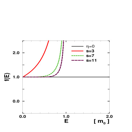
Figure 2: Cutoff factor $f(E)$ for $s=3+4n$ with $\eta=1[m_{0}^{2-s}]$.

For $s=1$ Ohmic dissipation, since $f(E)\to 0$ as $E\to 0$ and $f(E)\to 1$ as $E\to\infty$, the dissipation term $\Delta S_{\rm NL}$ suppresses the propagation in the $E\to 0$ region, that is, it is equivalent to an effective infrared cutoff. On the other hand, for $s=1+4n$ super-Ohmic dissipation, the propagation is suppressed in the $E\to\infty$ region, and the dissipation term $\Delta S_{\rm NL}$ is equivalent to an effective ultraviolet cutoff. These cutoffs have their own typical energy scales $E_{c}={\eta}^{-1/(s-2)}$ where $f(E)=\frac{1}{2}$.

Next, we consider the cases of $s=3+4n$ super-Ohmic dissipation shown in Fig. 2. In these cases $f(E)$ shows singular behavior in that it diverges at the energy scale $E_{c}={\eta}^{-1/(s-2)}$. This means that the theory is normal only below the ultraviolet cutoff energy $E_{c}$. In the normal region $f(E)$ is larger than $1$ and the propagation is enhanced.

As discussed above, $\Delta S_{\rm NL}$ acts as various types of effective cutoffs, which suppress or enhance the quantum fluctuation in energy dependent ways.

The NPRG method we employ now is a method to divide the variables $q(\tau)$ into energy shell modes, and to evaluate the quantum fluctuation of each shell mode systematically from the higher energy modes. It is suitable for studying the energy dependent cutoff effect appearing in dissipative quantum mechanics. Through the NPRG analysis of ordinary ($\eta=0$) quantum mechanics, we know that the effective energy region where the quantum fluctuations are significant depends on the mass scale of the theory ahtt . This fact implies that, if the cutoff effect originating from the dissipative term $\Delta S_{\rm NL}$ is large in this effective energy region, it may modify the phase structure of the system. In this way, the NPRG method allows us to understand intuitively the effect of $\Delta S_{\rm NL}$ as an effective energy dependent cutoff and discuss its strength by comparing it with the effective energy region of the original system. Such a viewpoint is a unique advantage of the NPRG approach.

IV Analysis of Dissipative Quantum Tunneling

IV.1 Macroscopic quantum coherence

The Caldeira-Leggett model consists of two classes of variables, the target system $q$ and the environmental degrees of freedom $\{x_{\alpha}\}$. We regard the system variable $q$ as a macroscopic collective coordinate and discuss how the quantum mechanical behavior of the macroscopic coordinate $q$ is affected by the environmental effects. As a typical phenomenon, the quantum tunneling of $q$ has been analyzed by many authors cl1 ; cl2 ; fiss1 ; fiss2 ; cha ; bm . We set the bare potential of $q$ as the double well type, $V_{0}(q)=-\frac{1}{2}q^{2}+\lambda_{0}q^{4}$. In this system with vanishing $\eta$ the $q$ mode tunnels through the potential barrier and oscillates between the two wells. The main question is whether or not it also oscillates even in the $\eta\neq 0$ dissipative system. Such an oscillatory behavior is called macroscopic quantum coherence and the inclination to cease the oscillation corresponds to decoherence weiss .

Now we briefly summarize the previous results obtained for macroscopic quantum coherence in double well potential systems with various types of dissipation $J(\omega)=\eta~{}\!\omega^{s}$. Usually the first energy gap $\Delta E=E_{1}-E_{0}$ is calculated as the physical quantity because it corresponds to the tunneling amplitude between the two wells. For $s=1$ Ohmic dissipation, Caldeira and Leggett evaluated it by using the semi-classical (instanton) approximation, which is valid for $\lambda_{0}\to 0$ and perturbation with respect to $\eta$, and they found that the dissipation $\Delta S$ suppresses the tunneling cl1 ; cl2 . Renormalization-group analyses have been done for the instanton gas system within the dilute gas approximation, which is also valid for $\lambda_{0}\to 0$ and $\eta\to 0$ cha ; bm . They predict the remarkable phenomenon that $\Delta E$ vanishes at a critical value $\eta_{c}=2\pi\lambda_{0}$, where decoherence occurs. This is often called the quantum-classical transition because the system looks classical in the limited sense that quantum tunneling does not occur. This is nothing but the spontaneous $Z_{2}$ symmetry breaking. The energy gap $\Delta E$ plays an important role as the order parameter of the transition.

On the other hand, for $s=3$ super-Ohmic dissipation, the possible enhancement of $\Delta E$ is shown by perturbative calculus with respect to $\eta$ in the canonical formulation fiss1 ; fiss2 . This result is interpreted as the effect of the higher excited states ($E_{n},n\geq 2$), and it cannot be reproduced by the standard instanton calculus. For the cases of $s=5,7,9,...$ super-Ohmic dissipation, no detailed analyses have been carried out. The dissipation effects in these cases are expected to be weak by simple power counting, since they are irrelevant in the infrared region.

These results we listed above are obtained by using the semiclassical approximation and/or perturbation theory with respect to $\eta$. Their reliability depend on the smallness of the couplings $\lambda_{0}$ and $\eta$. Therefore, to get more general and reliable results free of this limitation, we must employ an analyzing tool which does not need a series expansion with respect to any couplings. We expect our method of using the NPRG will work best, particularly for the large coupling region.

IV.2 NPRG analysis

We analyze dissipative quantum tunneling by solving the NPRG equation (27) numerically. This equation is a two-dimensional partial differential equation for the Wilsonian effective potential $V_{\Lambda}(q)$ with respect to $\Lambda$ and $q$. The initial condition of the potential is the bare potential $V_{\Lambda_{0}}(q)=-\frac{1}{2}q^{2}+\lambda_{0}q^{4}$ at the initial cutoff $\Lambda_{0}$. We solve the differential equation in the infrared limit $\Lambda\to 0$ and obtain the physical effective potential $V_{\rm eff}(q)$. The typical change of the potential toward the infrared is shown in Fig. 3. We see two basic features of the flow. The potential at the origin moves up, which finally gives the ground state energy of the zero point oscillation. The second derivative of the potential at the origin also increases from negative to positive, changing the potential form from a double well to a single well.

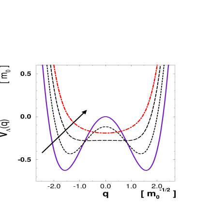
Figure 3: Flow of the potential for $\lambda_{0}=0.1[m_{0}^{3}]$.

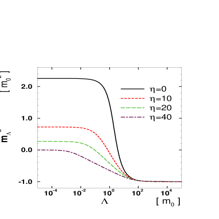
Figure 4: Running of $m^{2}_{\Lambda}$ for $\lambda_{0}=1.0[m_{0}^{3}]$. All values of $\eta$ are measured in units of $[m_{0}]$.

We note here the actual treatment of the infrared and the ultraviolet limit in the numerical calculation. The Wilsonian effective potential changes toward the infrared and finally stops changing at some finite scale of $\Lambda$, below which the quantum fluctuations are suppressed due to the mass of the system. Therefore before lowering the scale $\Lambda$ to vanishing, we get the infrared limit results. As for the initial cutoff, it should be infinite since the target system is quantum mechanics without an ultraviolet energy cutoff. We start with a large value of the initial cutoff to solve the equation, and check that the physical results given by the infrared potential change little when we move the initial cutoff up further. Then we regard our numerical results as those without any cutoff.

We can exploit the physical information of the quantum system from $V_{\rm eff}(q)$. First of all, the mass squared starting with a negative value $(-1)$ finally reaches a positive value (for small $\eta$), $m_{\rm eff}^{2}>0$, that is, the effective potential $V_{\rm eff}(q)$ becomes a single well form. The running of the mass squared is plotted in Fig. 4 for $\lambda_{0}=1.0$. This means that, due to the quantum tunneling, the $Z_{2}$ symmetry (parity) does not break spontaneously, and the expectation value of $q$ vanishes. The tunneling effects are automatically incorporated when we integrate (solve) the NPRG equation toward the infrared.

When the dissipation effects are included, the quantum propagator may be suppressed, and then such running of $m^{2}_{\Lambda}$ as shown in Fig. 4 is also suppressed. If the running is not enough, the mass squared may not become positive even at the infrared limit. This indicates spontaneous symmetry breaking, and localization should be observed.

For nonvanishing $\eta$, the correspondence between the energy gap $\Delta E$ and the effective mass $m_{\rm eff}$ Eq. (25) does not hold. The long range ($\tau\to\infty$) behavior of the two point function

$$\lim_{\tau\to\infty}\int\frac{dE}{2\pi}e^{iE\tau}\frac{1}{E^{2}+\eta|E|+m^{2}_{\rm eff}}$$ (30)

is actually independent of $m_{\rm eff}$ and is determined by $\eta$ with power damping behavior even in the case of infinitesimal $\eta$. This singular behavior comes from the nature of the environmental degrees of freedom where the harmonic oscillator frequencies are assumed to be distributed continuously up to zero ($\omega_{\alpha}=0$). Even if there is an infrared cutoff, it does not change the situation much and the lowest frequency environment dominates the long range correlator of the target system. In this sense semiclassical arguments depending on the long range transition amplitude seem doubtful for the purpose of investigating the localization transition.

Here, instead of analyzing the long range correlator, we adopt another physical quantity to describe the possible quantum-classical transition, the localization susceptibility. We suppose that a source term $J$ that couples to the zero mode of $\tilde{q}(E)$,

$$\tilde{q}(0)=\int^{T/2}_{-T/2}q(\tau)d\tau,$$ (31)

is included in the quantum action. Then the localization susceptibility $\chi$ is defined by

$$\chi\equiv\frac{1}{T}\left.\frac{d\langle\tilde{q}(0)\rangle_{J}}{dJ}\right|_{J=0}=\frac{1}{T}\left.\frac{d^{2}\ln Z}{dJ^{2}}\right|_{J=0},$$ (32)

and it is exactly given by the effective potential as follows:

$$\chi=\left(\frac{d^{2}V_{\rm eff}(q)}{dq^{2}}\right)^{-1}=\frac{1}{m^{2}_{\rm eff}}.$$ (33)

These definitions are valid also for nonvanishing $\eta$. If we find a divergent and scaled behavior of $\chi$ toward $\eta=\eta_{c}$, we may conclude that the localization transition occurs at $\eta_{c}$ and it is a second order phase transition.

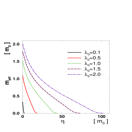
Figure 5: The effective mass $m_{\rm eff}$ for $s=1$ with initial cutoff $\Lambda_{0}=10^{4}[m_{0}]$. All values of $\lambda_{0}$ are measured by $[m_{0}^{3}]$ unit.

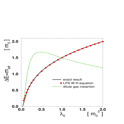
Figure 6: Energy gap estimates without dissipation.

The results for $s=1$ Ohmic dissipation are shown in Fig. 5 for several $\lambda_{0}$. In previous works ahtt ; kt ; za for the $\eta=0$ system, the NPRG analyses have been found to work excellently in these $\lambda_{0}$ regions while the dilute gas instanton approximation does not work at all there. In Fig. 6 we recapitulate the results for the energy gap with $\eta=0$ where those by the dilute gas instanton are also plotted for comparison and the exact values are calculated by solving the Schrödinger equation. We see that for the large $\lambda_{0}$ region ($\lambda_{0}\raisebox{0.86108pt}{$\ >\kern-10.50005pt\raisebox{-4.73611pt}{$\sim$}\ $}0.1$) the NPRG results looks excellent while the instanton method is out of its effective range just as is expected. Therefore we expect that the NPRG analysis also works well for these $\lambda_{0}$ values even in $\eta\neq 0$ systems.

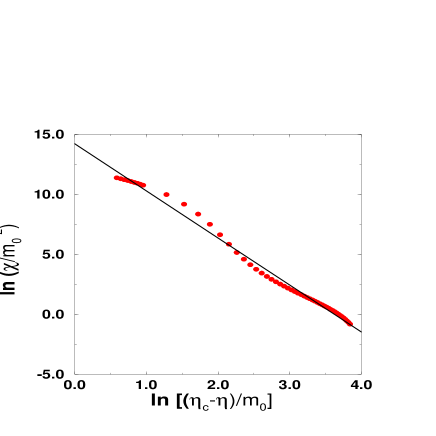
Figure 7: Critical scaling fit of localization susceptibility $\chi$ for $\lambda_{0}=1.0[m_{0}^{3}]$.

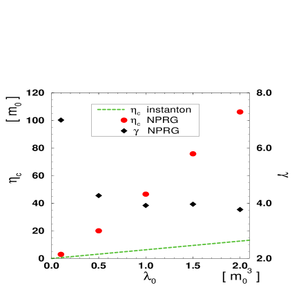
Figure 8: $\lambda_{0}$ dependence of critical dissipation $\eta_{c}$ and critical exponent $\gamma$.

We find that for every value of $\lambda_{0}$ $m_{\rm eff}$ decreases as $\eta$ becomes large (Fig. 5). This $\eta$ and $\lambda_{0}$ dependence of $m_{\rm eff}$ is readily understandable by using the property of the cutoff interpretation of the Ohmic dissipation. Remember that the quantum fluctuation of $q$ is suppressed below the effective infrared cutoff $E_{c}=\eta$. Therefore a larger $\eta$ causes a stronger cutoff effect and results in a smaller $m_{\rm eff}$. For larger $\lambda_{0}$, the system mass scale is larger, and therefore a larger $\eta$ is required to effectively cut off the quantum fluctuation. These behaviors are qualitatively consistent with those of $\Delta E$ obtained by the instanton approximation.

Then, what happens for larger $\eta$? The expected phenomenon is the quantum-classical transition characterized by complete disappearance of the tunneling. The NPRG method may not work precisely in the $m_{\rm eff}\to 0$ region because Eq. (27) becomes singular there and the numerical error increases. Therefore according to the standard technique of analyzing critical phenomena, we evaluate the critical dissipation $\eta_{c}$ from the diverging behavior of the localization susceptibility. We fit $\chi(\eta)$ with the critical exponent form

$$\chi=C|\eta-\eta_{c}|^{-\gamma}.$$ (34)

We show an example of fit for $\lambda_{0}=1.0$ in Fig. 7. We conclude that the localization susceptibility shows divergent behavior with a power scaling, which indicates a second order phase transition of localization, often called the quantum-classical transition.

We obtain the critical dissipation $\eta_{c}$ and the critical exponent $\gamma$ for these $\lambda_{0}$, which are plotted in Fig. 8. The previous analysis using the dilute gas instanton gives a simple relation $\eta_{c}=2\pi\lambda_{0}$ which is also shown in Fig. 8 for comparison. The NPRG results for $\eta_{c}$ are systematically large compared to those of the instanton. As for the critical exponent $\gamma$, we observe the universality property except for the smallest $\lambda_{0}=0.1$, where NPRG results may not be reliable.

Next we see the difference among various dissipation effects at $s=1,3,5$. The results for $\lambda_{0}=0.4$ are shown in Fig. 9 (for small $\eta$) and Fig. 10 (for large $\eta$). For small $\eta$, suppression ($s=1,5$) and enhancement (s=3) of quantum fluctuations are seen as we expect. Note that for the $s=3$ case, since the hard ultraviolet cutoff $E_{c}={1}/{\eta}$ exists, the theory is an effective theory defined only below the energy scale $E_{c}={1}/{\eta}$. Here we use the bare cutoff $\Lambda_{0}=100$, and the $s=3$ result can be obtained only in the region $0\leq\eta\leq 0.01$. If the system is analyzed perturbatively ($\eta\to 0$), such a hard cutoff problem is not recognized fiss1 ; fiss2 .

Let us compare the super-Ohmic ($s=5$) case with the Ohmic case. Both cases suppress the quantum fluctuation and the relative strength of the effects depends on $\eta$, which turns over at $\eta\sim 3.0$ as seen in Fig. 10. This turnover is explained by comparing the effective cutoff scale due to dissipation $E_{c}=\eta^{-1/(s-2)}$ with the original mass scale of the system determined by $m_{0}$ and $\lambda_{0}$.

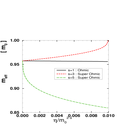
Figure 9: Dissipation dependence of $m_{\rm eff}$ for $\lambda_{0}=0.4[m_{0}^{3}]$ with initial cutoff $\Lambda_{0}=100[m_{0}]$ in the small $\eta$ region. We divide $\eta$ by $m_{0}^{2-s}$ in order to make it dimensionless.

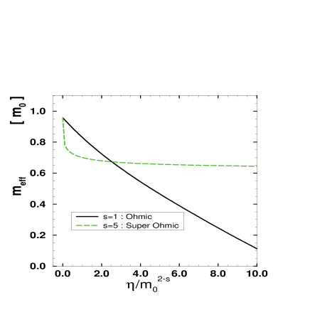
Figure 10: Dissipation dependence of $m_{\rm eff}$ for $\lambda_{0}=0.4[m_{0}^{3}]$ with initial cutoff $\Lambda_{0}=100[m_{0}]$ in the large $\eta$ region.

How about the possibility of the quantum-classical transition with super-Ohmic dissipation ($s=5,9,...$)? Contrary to the Ohmic case, the dissipation effect corresponds to the effective ultraviolet cutoff with scale $E_{c}={\eta}^{-1/(s-2)}$. Taking account of the basic notion that the infrared energy region is most significant for the localization transition, we may conclude that it is impossible for super-Ohmic dissipation to suppress quantum tunneling completely. This was expected from naive power counting, that is, the super-Ohmic dissipation is irrelevant in the infrared region.

V Summary and Discussion

We analyzed the Caldeira-Leggett model by the nonperturbative renormalization-group method. We derived the NPRG equation with a dissipation term characterized by $J(\omega)=\eta\omega^{s}$ within the local potential approximation. This method enables us to regard dissipation effects as various cutoff effects that enhance or suppress the quantum fluctuations of the system.

We applied the NPRG equation to analysis of macroscopic quantum coherence and investigated the quantum-classical transition due to dissipation. For Ohmic dissipation, we observed that the localization susceptibility $\chi$ diverges toward $\eta=\eta_{c}(\lambda_{0})$ with critical scaling, and we concluded that $\eta_{c}(\lambda_{0})$ is the critical dissipation for the quantum-classical transition. There must remain, however, many fundamental and subtle problems to be studied about the notion of the quantum-classical transition and critical dissipation.

In this article we did not consider the origin of the environmental degrees of freedom. It is very interesting to regard some higher dimensional fields as an environment coupled to quantum mechanical particles and to study how to treat such a complex system by the NPRG method. Furthermore, it not clear how to discriminate or construct the target macroscopic collective coordinate among the microscopic degrees of freedom. The NPRG method best fits the purpose of identifying the macroscopic effective theory for slow motion by averaging the quantum fluctuations.

- (1) A. O. Caldeira and A. J. Leggett, Phys. Rev. Lett. 46, 211 (1981).
- (2) A. O. Caldeira and A. J. Leggett, Annals Phys. 149, 374 (1983).
- (3) K. Fujikawa, S. Iso, M. Sasaki and H. Suzuki, Phys. Rev. Lett. 68, 1093 (1992).
- (4) K. Fujikawa, S. Iso, M. Sasaki and H. Suzuki, Phys. Rev. B46, 10295 (1992).
- (5) S. Chakravarty, Phys. Rev. Lett. 49, 681 (1982).
- (6) A. J. Bray and M. A. Moore, Phys. Rev. Lett. 49, 1545 (1982).
- (7) M. P. A. Fisher and W. Zwerger, Phys. Rev. B32, 6190 (1985).
- (8) U. Weiss, Quantum Dissipative Systems, 2nd ed. (World Scientific, Singapore 1999).
- (9) R. Fazio and H. van der Zant, Phys. Rep. 355, 235 (2001).
- (10) K. G. Wilson and J. B. Kogut, Phys. Rep. 12, 75 (1974).
- (11) F. Wegner and A. Houghton, Phys. Rev. A8, 401 (1973).
- (12) A. Hasenfratz and P. Hasenfratz, Nucl. Phys. B270, 687 (1986).
- (13) T. R. Morris, Prog. Theor. Phys. Suppl. 131, 395 (1998).
- (14) K.-I. Aoki, Prog. Theor. Phys. Suppl. 131, 129 (1998).
- (15) K.-I. Aoki, Int. J. Mod. Phys. B14, 1249 (2000).
- (16) K.-I. Aoki, A. Horikoshi, M. Taniguchi and H. Terao, in The Exact Renormalization Group (World Scientific, Singapore 1999), p. 194.
- (17) A. S. Kapoyannis and N. Tetradis, Phys. Lett. A276, 225 (2000).
- (18) D. Zappala, Phys. Lett. A290, 35 (2001).
- (19) K.-I. Aoki and A. Horikoshi, e-print quant-ph/0204078.
- (20) A perturbative renormalization-group analysis has been done for dissipative quantum mechanics with periodic potential and an interesting localization-delocalization transition has been discovered fz .
- (21) In this paper we use the term “mass” in the sense of quantum field theory, that is, the mass of the exciton.