Laser-driven atom moving in a multimode cavity: strong enhancement of cavity-cooling efficiency

Abstract

Cavity-mediated cooling of the center–of–mass motion of a transversally, coherently pumped atom along the axis of a high–Q cavity is studied. The internal dynamics of the atomic dipole strongly coupled to the cavity field is treated by a non-perturbative quantum mechanical model, while the effect of the cavity on the external motion is described classically in terms of the analytically obtained linear friction and diffusion coefficients. Efficient cavity-induced damping is found which leads to steady-state temperatures well-below the Doppler limit. We reveal a mathematical symmetry between the results here and for a similar system where, instead of the atom, the cavity field is pumped. The cooling process is strongly enhanced in a degenerate multimode cavity. Both the temperature and the number of scattered photons during the characteristic cooling time exhibits a significant reduction with increasing number of modes involved in the dynamics. The residual number of spontaneous emissions in a cooling time for large mode degeneracy can reach and even drop below the limit of a single photon.

I Introduction

The mechanical effect of light on atoms in high-Q cavities is currently being the subject of intensive theoretical and experimental research. The large interest that this field attracts is due to the complexity of the strongly-coupled dynamics of a moving atom and a few-photon field, as compared to the relatively well-understood atomic motion in external laser fields. Various effective cooling and trapping schemes have recently been found, which can drive atoms to low, sub-Doppler temperatures on a fast time scale. The use of dynamical fields in optical cavities is also a promising approach to extend the power of ordinary laser cooling methods to a large variety of atomic species. There are cooling mechanisms independent of the internal electronic structure of the particle, which could enable us to achieve the principal goal of cooling molecules.

In the simplest cavity-cooling schemes mossberg ; lewenstein ; cirac ; vuletic99 ; vuletic01 the cavity is used as a passive element to taylor the atomic spontaneous emission rate by altering the spectral mode density. For example, in the pioneering work by Mossberg et al. mossberg , an atom moving in a resonant laser standing-wave field can undergo a Sisyphus-type cooling in coloured vacuum, e.g. the one created inside a cavity. The spontaneous emission is then favoured, by selection in frequency space, from the top of a potential hill into the bottom of a potential well. Similarly, Vuletić et al.  vuletic01 pointed out that a two-photon Doppler-effect can occur provided the atom tends to scatter inelastically an incoming laser photon into a cavity mode of higher resonance frequency.

Dynamic cavity-cooling effects have been first predicted in Refs. horak97 ; hechenblaikner98 . In these schemes the free atom moves in a weakly driven cavity field. The damping relies on a strongly coupled atom-field system, in which the field exhibits non-adiabatic dynamics due to the finite mode bandwidth $\kappa$. Let us emphasize that the cooling mechanism is quite sophisticated, requiring at least two elements: (i) strong atom-field coupling manifested by the dressed state spectrum of the atom-cavity system; (ii) a cavity bandwidth in a specific narrow parameter range for the non-conservative dynamics. Both conditions are present in current setups pinkse00 ; hood00 and indications of the predicted mechanical effects have been observed in experiments.

In this paper we will consider nonadiabatic effects in a configuration similar to the ones in Refs. mossberg ; lewenstein ; vuletic99 ; vuletic01 , that is, a moving atom is driven by a classical laser field from the side, and cavity photons are created only via the atom, by scattering from the laser field. We proceed in two respects. First, we move towards the strong coupling regime where the non-conservative dynamical effects, analogous to the ones explored in Refs. horak97 ; hechenblaikner98 , appear and amount to new cooling regimes in the parameter space. Accordingly, we will present a non-perturbative quantum treatment of the internal dynamics of the coupled atom-cavity system. Our model is exact in the low-saturation regime that happens either for large atomic detuning or for weak external driving intensity. The diffusion coefficient due to dipole heating and the linear friction coefficient will be analytically calculated, which allows for the statistical description of the center-of-mass (CM) motion characteristics. We obtain the somewhat surprising result that pumping the atomic or pumping the field component of the coupled system are not the same even for low saturation. Although the similarity appears in the form of a quite intuitive symmetry between the results we derive and the ones presented in Refs. horak97 ; hechenblaikner98 for the cavity-driven system, important physical differences follow from the two different situations. Such consequences can be found, for example, in the temperature dependence on the system parameters.

As a second step forward, we will study multimode effects of the cavity-induced forces. Multimode fields have been conjectured to give rise to a significant improvement in terms of steady-state temperature when many cavity modes are driven simultaneously horak01 , and also in the case of the two-photon Doppler effect vuletic01 . In the physical configuration we consider in this paper, the only component of the system being externally driven is the atom. It is a very natural and, in practice, a simple extension to put a multimode cavity, such as a confocal resonator, around the driven particle. We ask what happens if there are several modes interacting with the atomic dipole. Here we will concentrate on scaling laws rather than on the geometrical aspects of the multimode cavity field, this latter is being important, e. g., to reveal atomic trajectories kaleidoscope . We consider degenerate modes with closely uniform mode functions. This situation proves to be an easy way to effectively enhance the dipole interaction strength and reach previously unexplored regimes of the dynamics. One of the main questions is if the number of spontaneously scattered photons during the cooling time can be restricted below the single photon level, which is the necessary requirement for effectively cooling particles without closed two-level pumping cycle.

The paper is organized as follows. In Sect. 2 we present the model of the system, and introduce the definition of the mechanical forces and the diffusion that we use to describe the semiclassical CM motion. In Sect. 3 the set of linearized Heisenberg–Langevin equations is solved which leads to the analytical expressions for the linear friction and the diffusion coefficients. These results are analyzed first for a single-mode cavity in Sect. 4, with the aim of identifying the cooling mechanisms relying on a passive cavity and those originating from the strongly-coupled atom-cavity dynamics. Then, in Sect. 5., we study how the physically relevant quantities, such as the steady-state temperature, the cooling time, and the number of spontaneously scattered photons scale with the number of degenerate modes of a multimode cavity. Finally, we conclude in Sect. 6.

II The model

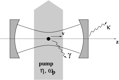
Figure 1: Schematic representation of the system composed of a cavtity and a moving atom that is driven from the side.

The system is composed of $M$ degenerate modes of a high-finesse cavity interacting with a moving atom. The atom is driven from the side by a coherent laser field (see Fig. 1). We restrict the study of the atomic motion to the longitudinal dimension along the cavity axis. The driving field can be assumed uniform in the relevant range of the atomic motion. This is equivalent to neglecting the slow variation of the Gaussian envelope which is broad compared to the wavelength. The pumping strength is thus given by a single parameter $\eta$. The pumping frequency $\omega_{p}$ is detuned from the atomic transition frequency with $\Delta_{A}=\omega_{p}-\omega_{A}$ and from the common resonance frequency of the modes with $\Delta_{C}=\omega_{p}-\omega_{C}$. The dipole-cavity field interaction is described by the Hamiltonian

$$H=-\hbar\Delta_{C}\sum_{i=1}^{M}a_{i}^{\dagger}a_{i}-\hbar\Delta_{A}\sigma^{\dagger}\sigma-i\hbar\eta(\sigma-\sigma^{\dagger})\\ -i\hbar\sum_{i=1}^{M}[g_{i}(z)\sigma^{\dagger}a_{i}-g_{i}^{*}(z)a_{i}^{\dagger}\sigma]\;,$$ (1)

which is written in a frame rotating at the pumping frequency $\omega_{p}$. The atomic dipole operator is denoted by $\sigma$, and $a_{i}$ is the bosonic field-amplitude operator associated with the $i$th mode. The position-dependent dipole coupling is $g_{i}=\sqrt{\hbar\omega_{C}/2\epsilon{\cal V}_{i}}\,d\,f_{i}(z)$, where $d$ is the atomic dipole moment, ${\cal V}_{i}$ is the effective volume of the mode $i$, and $f_{i}(z)$ is the respective mode function which is normalized to have the maximum equal to 1.

In addition to this coherent dynamics, the system is subject to dissipation processes, i.e. to spontaneous emission with rate $2\gamma$ into radiation modes other than the cavity ones, and to cavity photon loss with a uniform rate of $2\kappa$ for all the degenerate modes. The resulting open system can be described by Heisenberg–Langevin equations. We consider the low-saturation regime where the atomic population inversion operator $\sigma_{z}=(\sigma^{\dagger}\sigma-\sigma\sigma^{\dagger})/2$ can be replaced by the c-number $-1/2$. With this approximation one gets a linear set of equations

$$\dot{\sigma} =(i\Delta_{A}-\gamma)\sigma-\sum_{i=1}^{M}g_{i}(z)a_{i}+\eta+\xi_{A}$$ (2a)

$$\dot{a}_{i} =(i\Delta_{C}-\kappa)a_{i}+g_{i}^{*}(z)\sigma+\xi_{i}\;,$$ (2b)

for all the modes $i=1..M$. The Langevin noise operators are defined by the second-order correlations

$$\langle\xi(t_{1})\xi^{\dagger}(t_{2})\rangle =2\gamma\,\delta(t_{1}-t_{2})$$ (3a)

$$\langle\xi_{i}(t_{1})\xi_{j}^{\dagger}(t_{2})\rangle =2\kappa\,\delta_{ij}\,\delta(t_{1}-t_{2})\;,$$ (3b)

all the other correlations vanish. Note that a simple transformation, $\sigma\rightarrow\sigma-\eta/(i\Delta_{A}-\gamma)$ shifts the driving from the atomic dipole $\sigma$ to the mode amplitudes $a_{i}$, thus one could think that driving the field and driving the atomic component leads to equivalent dynamics. However, this is not true for a moving atom when $z$ is considered also as a variable.

In the Heisenberg–Langevin equations of the field amplitudes and the atomic dipole, the atomic position appears as a parameter. Nevertheless, under the mechanical effect of the radiation field on the atomic center–of–mass motion, the atomic position is also a variable. In the present paper we use a consistent semiclassical model that relies on a classical treatment of the CM motion cohen92 . The external atomic CM dynamics is assumed to decouple from the internal one given by the Eqs. (2), and it is governed by a Langevin-type equation

$$\dot{x} =p/m$$ (4a)

$$\dot{p} =f_{p}+\beta p+\xi_{p}\;,$$ (4b)

where $f_{p}$ is a conservative force, $\beta$ is a friction coefficient and $\xi_{p}$ is a classical stochastic term giving rise to diffusion. Statistical properties of the CM motion can be derived from this Langevin-equation. This semiclassical approach is consistent as long as the temperature is far above the recoil temperature $T_{\mbox{\tiny rec}}=\hbar^{2}k^{2}/2m$, where $k$ is the wave number of the modes involved, $m$ is the mass of the atom.

The aim of the present paper consists in calculating the coefficients in Eq. (4b). They all can be derived from the force operator, which is given by the gradient of the interaction term in the Hamiltonian cohen92

$$F=i\hbar\sum_{i=1}^{M}[(\partial_{z}g_{i})\sigma^{\dagger}a_{i}-(\partial_{z}g_{i}^{*})a_{i}^{\dagger}\sigma]\;.$$ (5)

First, the mean of the force operator provides directly $f_{p}$,

$$f_{p}=\langle F\rangle\;.$$ (6)

Then, the noise term $\xi_{p}$ originates from the fluctuations of the force operator. On evaluating the two-time correlation function,

$$\langle F(t_{1})F(t_{2})\rangle-\langle F(t_{1})\rangle\langle F(t_{2})\rangle={\cal D}_{p}\,\delta(t_{1}-t_{2})\;,$$ (7)

the momentum diffusion coefficient can be identified with the coefficient of the function $\delta(t_{1}-t_{2})$. Note that here we use a different approach to the diffusion coefficient as compared to earlier work horak97 ; hechenblaikner98 ; cohen92 ; domokos01 . It has the additional advantage that the motional diffusion is linked directly to the quantum noise accompanying the dissipation processes of the system, i.e., the dipole fluctuations due to spontaneous emission ($\xi_{A}$ that scales with $\gamma$) and the cavity photon loss ($\xi_{i}$ that scales with $\kappa$). It allows to reveal how the basic noise sources of the internal dynamics yield diffusion of the external CM motion.

Finally, for the friction coefficient $\beta$, the dependence of the internal variables $a_{i}$ and $\sigma$ on the velocity has to be taken into account. Indeed, the non-conservative friction force arises from the time-delayed reaction of the internal variables to the displacement of the atom. They require a period of $\kappa^{-1}$ or $\gamma^{-1}$ (in the coupled system typically the shorter time, though this depends also on the coupling strength) to reach the stationary state adapted to the actual position of the atom. If the atom moves much less than the wavelength during this time, i.e. in the low-velocity limit $kv\ll\gamma,\kappa$, the velocity-dependence of the variables can be taken into account in a consistent way. The time derivative is to be replaced by $d/dt\rightarrow\partial/\partial t+v\partial/\partial x$ and, simultaneously, the variables are expanded into the series

$$\sigma =\sigma^{(0)}+v\sigma^{(1)}+{\cal O}(v^{2})$$

$$a_{i} =a_{i}^{(0)}+va_{i}^{(1)}+{\cal O}(v^{2})\;.$$

The resulting dynamical equations can be solved systematically in different orders of the velocity $v$. The first order components obey the set of linear equations

$$(i\Delta_{A}-\gamma)\sigma^{(1)}-\sum_{i=1}^{M}g_{i}(z)a_{i}^{(1)}=\partial_{z}\sigma^{(0)}$$ (8a)

$$(i\Delta_{C}-\kappa)a_{i}^{(1)}+g_{i}^{*}(z)\sigma^{(1)}=\partial_{z}a_{i}^{(0)}\;,$$ (8b)

The coefficient $\beta$ of the linear friction force can be defined as

$$\beta/m=\langle F^{(1)}\rangle=i\hbar\sum_{i=1}^{M}(\partial_{z}g_{i})\langle{\sigma^{\dagger}}^{(0)}a_{i}^{(1)}+{\sigma^{\dagger}}^{(1)}a_{i}^{(0)}\rangle-\mbox{H.c.}\;.$$ (9)

III Solving the linear system

In this section we perform the calculation of the linear friction and the diffusion coefficients by directly solving the equations describing the internal dynamics, i.e. Eqs. (2) and (8). Let us introduce the Fourier transform of the operators,

$$O(t)=\frac{1}{\sqrt{2\pi}}\int_{-\infty}^{\infty}d\Omega e^{-i\Omega t}O(\Omega)$$ (10)

and use the rule $\partial/\partial t\rightarrow-i\Omega$. The velocity-independent part of the system variables yields

$$\sigma^{(0)}(\Omega) =\frac{1}{D(\Omega)}\left[(\kappa-i\Delta_{C}-i\Omega)(\sqrt{2\pi}\delta(\Omega)\eta+\xi_{A}(\Omega))-\sum_{k=1}^{N}g_{k}(z)\xi_{k}(\Omega)\right]\;,$$ (11a)

$$a_{i}^{(0)}(\Omega) =\frac{1}{D(\Omega)}\left[g_{i}^{*}(z)(\sqrt{2\pi}\delta(\Omega)\eta+\xi_{A}(\Omega))+\frac{D(\Omega)}{\kappa-i\Delta_{C}-i\Omega}\xi_{i}(\Omega)-\sum_{k=1}^{N}\frac{g_{i}^{*}(z)g_{k}(z)}{\kappa-i\Delta_{C}-i\Omega}\xi_{k}(\Omega)\right]\;,$$ (11b)

where the determinant of the linear system reads

$$D(\Omega)=(\kappa-i\Delta_{C}-i\Omega)(\gamma-i\Delta_{A}-i\Omega)+\sum_{k=1}^{N}|g_{k}(z)|^{2}\;.$$ (12)

The system variables are obtained as linear combinations of the pumping term $\eta$ and noise operators. Note that, as a consequence of the coupled dynamics, both the field-amplitude operators $a_{i}$ and the dipole operator $\sigma$ incorporate the fluctuations $\xi_{A}$ and $\xi_{i}$, associated with the spontaneous emission and from the cavity photon loss, respectively.

In any normal-ordered expression of the operators $a_{i}^{\dagger}$, $\sigma^{\dagger}$, $\sigma$, and $a$, all the noise operators $\xi$ are found on the right side, while all the adjoint operators $\xi^{\dagger}$ occur on the left side of the expression. Therefore, when evaluating the mean value of a normal-ordered product, the noise terms have no contribution. It is useful to introduce the c-number variables which arise from the coherent driving terms of the exact expression (11). They correspond to the stationary solution of a semiclassical model of the same system, and read

$$s^{(0)} =\eta\frac{\kappa-i\Delta_{C}}{D}\;,$$ (13a)

$$\alpha_{i}^{(0)} =\eta\frac{g_{i}^{*}(z)}{D}\;,$$ (13b)

where, and hereafter in the paper, $D=D(0)$. In normal-ordered products, the operators can be replaced by these simple “semiclassical” solutions. For example, the atomic excitation is obtained as

$$\langle{\sigma^{\dagger}}^{(0)}\sigma^{(0)}\rangle={s^{(0)}}^{*}s^{(0)}=\eta^{2}(\kappa^{2}+\Delta_{C}^{2})/|D|^{2}\;,$$ (14)

which has to be well below one in order to be consistent with the low-saturation assumption. The steady-state photon number in the mode $i$ is

$$\langle{a_{i}^{\dagger}}^{(0)}a_{i}^{(0)}\rangle ={\alpha^{(0)}}^{*}\alpha^{(0)}=\eta^{2}|g_{i}(z)|^{2}/|D|^{2}$$

$$=\langle{\sigma^{\dagger}}^{(0)}\sigma^{(0)}\rangle\;|g_{i}(z)|^{2}/(\kappa^{2}+\Delta_{C}^{2})\;.$$ (15)

The second expression exhibits how the photon number is related to the atomic excitation. As this latter is necessarily small, the photon number has to be below $g/\kappa$.

III.1 The friction coefficient

The friction coefficient is defined, in Eq. (9), by a normally ordered expression. Hence, it is enough to take into account the coherent driving terms, i.e., the semiclassical solution (13) of the variables. Accordingly, the components, first-order in velocity, have to be determined from the Eqs. (8) by using only the c-number part of the solutions. This simplifying fact is in accordance with the physical intuition. The non-adiabatic dynamics of the internal variables, being the origin of the damping, does not substantially depend on the noise. On the other hand, the non-adiabaticity must be reflected in the dynamics of the c-number semiclassical variables, since it includes the pumping and damping processes of the coupled internal system.

The first-order components of the variables can be easily obtained. They are

$$s^{(1)} =\frac{\eta}{D^{3}}[(\kappa-i\Delta_{C})^{2}-G](\partial_{z}G)+\frac{\eta}{D^{2}}\Gamma$$ (16a)

$$\alpha_{i}^{(1)} =\frac{\eta}{D^{3}}(\kappa-i\Delta_{C}+\gamma-i\Delta_{A})g_{i}^{*}(\partial_{z}G)$$

$$\qquad-\frac{\eta}{D^{2}}\frac{1}{\kappa-i\Delta_{C}}\left(D(\partial_{z}g_{i}^{*})-g_{i}^{*}\Gamma\right)\;,$$ (16b)

where

$$G =\sum_{k=1}^{M}|g_{k}|^{2}$$ (17a)

$$\Gamma =\sum_{k=1}^{M}g_{k}(\partial_{z}g_{k}^{*})\;,$$ (17b)

Note that $(\partial_{z}G)=\Gamma+\Gamma^{*}$. Replacing these expressions into the definition (9), one gets the friction coefficient. Here we present only the solution for a standing-wave cavity, where the mode functions are real. It is

$$\begin{split}\beta=-&\hbar\frac{\eta^{2}}{|D|^{4}}(\partial_{z}G)^{2}\left[\kappa\Delta_{A}+2\Delta_{C}\left(\kappa+\gamma+\kappa\frac{\kappa\gamma-\Delta_{C}\Delta_{A}+G/2}{\kappa^{2}+\Delta_{C}^{2}}\right)\right]\\ +&4\hbar\frac{\eta^{2}}{|D|^{6}}(\partial_{z}G)^{2}\Delta_{C}(\kappa\Delta_{A}+\gamma\Delta_{C})[\kappa^{2}\Delta_{A}+\gamma^{2}\Delta_{C}+(\Delta_{A}+\Delta_{C})(\Delta_{A}\Delta_{C}-G)]\\ +&4\hbar\frac{\eta^{2}}{|D|^{2}}\frac{\kappa\Delta_{C}}{\kappa^{2}+\Delta_{C}^{2}}\sum_{k}(\partial_{z}g_{k})^{2}\end{split}$$ (18)

The generalization for running-wave modes in a ring cavity is straightforward.

III.2 Diffusion coefficient

The diffusion stems from the fluctuation of the force operator, i.e., that of the dipole interaction term of the Hamiltonian (1). When calculating the diffusion coefficient from its definition (7), the product of the force operators contains non-normally ordered terms. Hence, the noise terms in the solutions (11) have non-vanishing contributions, and the noise correlations given in (3) have to be used in the calculation. One can separate terms originating from the spontaneous emission noise ($\xi_{A}$) and from the cavity loss noise ($\xi_{i}$). We omit the details of the lengthy calculation here apart frommentioning one non-trivial step in the derivation. Although the sources $\xi_{A}$ and $\xi_{i}$ ($i=1...M$) are supposed to represent white noise, the resulting noise associated with the force operator becomes coloured, that is, it has a non-uniform spectrum. Accordingly, in addition to the Dirac-$\delta$ correlation assumed in the definition (7), one obtains other terms proportional to the derivatives of the Dirac-$\delta$ to all order. We neglect these terms and consider the coefficient of the Dirac-$\delta$ to describe the diffusion process.

The diffusion coefficient for real mode functions reads

$${\cal D}_{\mbox{\tiny dip}}=2\hbar^{2}\frac{\eta^{2}}{|D|^{2}}\Biggl{(}\kappa\sum_{k}\left(\partial_{z}g_{k}\right)^{2}\\ +(\partial_{z}G)^{2}\Delta_{C}\frac{\kappa\Delta_{A}+\gamma\Delta_{C}}{|D|^{2}}\Biggr{)}$$ (19)

In addition to the dipole heating, the noise induced by the random recoil accompanying the spontaneous emission has to be taken into account. The recoil contributes to the total diffusion by

$${\cal D}_{\mbox{\tiny rec}}=2\hbar^{2}k_{A}^{2}\bar{u^{2}}\frac{\eta^{2}}{|D|^{2}}(\kappa^{2}+\Delta_{C}^{2})\gamma\;,$$ (20)

where $k_{A}=\omega_{A}/c$ and $\bar{u^{2}}$, characteristic of the atomic transition, is the mean of the recoil momentum projected on the cavity axis.

To conclude this section let us emphasize that the results for the friction and the diffusion coefficients have a general validity regardless of the relationship of the parameters involved. The only condition is the weak atomic excitation that can always be met by a proper adjustment of the pumping strength $\eta$.

IV Cooling regimes

In this section we evaluate the previously calculated expressions for the diffusion and friction coefficients for a single-mode cavity. Such an analysis serves as a ground to identify the physical processes underlying the cavity-cooling. In addition, it is interesting to compare the results with those obtained in a similar system horak97 ; hechenblaikner98 with the cavity mode being driven instead of the atom.

There were several attempts to interpret the cooling in terms of simple physical processes, such as two-photon Doppler effect vuletic99 , or Sisyphus-effect in the dressed state basis hechenblaikner98 . In what follows, we propose to explore the friction mechanism by systematically varying the parameters, through relatively simple limiting cases to a final, quite general parameter setting in the strong-coupling cavity QED regime. In Figs. 2 and 3 the friction coefficient is shown as a function of the detunings in a contour plot style for various characteristic values $\kappa$ and $g$ of the cavity.

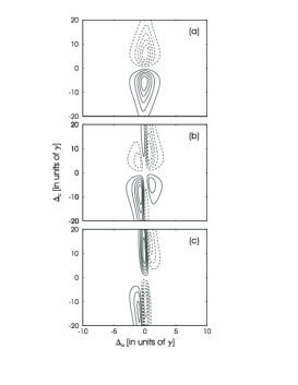
Figure 2: Contour plot of the friction coefficient in the bad-cavity regime ($\kappa=10\gamma$) for various coupling constants, (a) $g=\gamma/2$, (b) $g=3\gamma/2$, (c) $g=3\gamma$, linking the closely independent atom and cavity field system to the dressed atom one. Solid contour lines indicate cooling ($\beta<0$), dashed ones heating ($\beta>0$) regions.

Let us start in the bad-cavity limit with a negligibly small coupling parameter ($\kappa=10\gamma$, $g=\gamma/2$). This corresponds to the simple perturbative regime of cavity QED, where the role of the cavity is that it reshapes the radiative environment of the atom and increases the spontaneous emission rate at the cavity frequency. In our one-dimensional model we are interested in mechanical forces due to cavity photons. As these photons leak out of the cavity fast, such that no dynamics occur on a time scale longer than $\kappa^{-1}$, the atom-cavity field interaction can be basically considered as scattering. Although the atomic dipole is linear in the low-saturation regime, inelastic scattering can happen due to the CM motion that is able to compensate for the energy difference. For $\omega_{C}>\omega_{p}$, the spontaneous emission being favoured at the cavity frequency higher than the incoming one, the scattering is accompanied by a loss of the kinetic energy, i.e. cooling. This is the origin of the cooling region for $\Delta_{C}<0$ in Fig. 2a, and in turn, the same mechanism acts reversly leading to heating for $\Delta_{C}>0$. Note that this simple energy conservation argument is also in the heart of the interpretation given in vuletic01 for the two-photon Doppler effect.

Next, let us keep $\kappa$ large and increase gradually the coupling constant $g$. Figures 2b and c correspond to $g=1.5\gamma$ and $g=3\gamma$, respectively. Two sharp peaks emerge at $\Delta_{A}\approx 0$. As $\kappa$ is still the far largest parameter, the scattering picture applies. However, instead of the bare atom, the strongly coupled atom-cavity system has to be taken into account. As a consequence, relatively close to the pumping frequency $\omega_{p}$, the spectrum now exhibits the doublet of the first excited dressed-state manifold. Scattering of a pump photon into a cavity one may happen now via both intermediate states. In the case of $\Delta_{C}<0$ and $\Delta_{A}\approx 0$, for example, which is the lower half plane of the plots 2b and c, the upper dressed state $|+\rangle$ is at about the cavity frequency $\omega_{C}$ with a width of $\kappa$. The upper level therefore amounts to cavity photons of frequency about $\omega_{C}$, which corresponds to the process we described just before and is responsible for the broad cooling peak in the background. For large enough coupling constant, however, the lower state $|-\rangle$ is contaminated with a non-negligible amount of $|g,1\rangle$ component, its weight is proportional to $g^{2}/(\omega_{C}-\omega_{A})^{2}$. Pumping photons can then be transmitted into the cavity by exciting the lower dressed state at the frequency of about $\omega_{A}+2g^{2}/(\omega_{A}-\omega_{C})$. For $\Delta_{A}\approx 0$ this state is more resonant with the pump and the corresponding scattering channel becomes dominant. That is, one gets the heating peak for $\Delta_{C}<0$ and $\Delta_{A}>0$, whose width is approximately $\gamma$, the one of the lower dressed level. For $\Delta_{A}<0$ the driving field is tuned below the lower dressed level and thus scattering via this state yields cooling again. Note the displacement of the heating peak with respect to the axis $\Delta_{A}=0$ which is due to the cavity-vacuum induced lightshift, i. e., the lower dressed-state resonance and the atomic resonance do not coincide.

Regardless of the value of the coupling constant, as long as $g\ll\kappa$, the field adiabatically follows the atomic dynamics, as is the case for the parameter settings chosen for Fig. 2. The damping effect cannot be attributed to a non-conservative, time-delayed field dynamics. This kind of behaviour occurs when decreasing the cavity linewidth $\kappa$. Then, instead of being a passive element with specific mode density, it becomes necessary to include the cavity field as a dynamical component of the system. For longer spontaneous lifetimes, the system spends some time in the dressed states and the slow atom moves in a potential associated with the sinusoidally varying dressed levels.

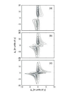
Figure 3: Contour plot of the friction coefficient in the dressed-atom regime ($g=3\gamma$) for decreasing cavity linewidth, (a) $\kappa=5\gamma$, (b) $\kappa=2\gamma$, (c) $\kappa=\gamma$, linking the adiabatic field dynamics regime to the one including time-delay, and the accompanying non-conservative cavity forces.

In Figs. 3a–c, the case of $\kappa=5\gamma$, $2\gamma$, and $\gamma$ are shown, respectively. There appears a pair of peaks with hyperbolic shape along $\Delta_{C}\Delta_{A}\approx g^{2}$, which is cooling for negative detunings $\Delta_{C},\Delta_{A}<0$, and heating for positive ones $\Delta_{C},\Delta_{A}>0$. This cooling (heating) region corresponds to the situation where the lower (upper) dressed state is resonantly pumped at antinodes (maximum coupling) and thus the slowly moving atom has to, on average, climb up potential hills (descend to potential valleys).

Finally, there are two peaks at at $\Delta_{C}\approx 0$ that can be attributed to the effect of the Doppler-shift in the correlated atom-field dynamics. Compared to the free-space Doppler cooling case, the preferential direction appears in the emission rather than in the absorption. For $\Delta_{A}>0$ and $\Delta_{C}\approx 0$, the atom gets closer to resonance with the copropagating component of the standing-wave field, i.e., following an emission the atom is more likely to impart a recoil in the direction opposite to its velocity.

One can expect that in the low-saturation regime, where the Heisenberg-Langevin equations are linearized, it makes no difference which component of the coupled system is being pumped. Indeed, this intuition is reflected in the mathematical form of the results. We checked that a systematic exchange of the parameters ($\Delta_{A}$, $\gamma$) $\leftrightarrow$ ($\Delta_{C}$, $\kappa$) in the expressions (18) and (19) reproduces the results obtained for the cavity-driven case in Ref. hechenblaikner98 . This symmetry reveals that the roles of the two oscillators, the field mode and the atomic dipole, are interchanged. Accordingly, the map of the friction coefficient in Fig. 3c is similar to the Fig. 3 of Ref. hechenblaikner98 with the detuning axes exchanged (reflection to the diagonal). In principle, for $\kappa=\gamma$ there is a one-to-one correspondence between the two systems, i.e. a given dynamics of the atom-driving configuration can be mimicked, with exchanged detunings $\Delta_{C}$ and $\Delta_{A}$, in the cavity-driving one. However, for a fixed setting of the detunings, the accompanying cooling (or heating) mechanism is different, which leads to an essential modification of the relevant physical quantities. This deviation becomes of importance when there is an additional constraint concerning the detunings, for example, $\Delta_{A}$ has to be very large to keep the spontaneous photon scattering low for molecule cooling. The more detailed analysis of this comparison is relegated into the next section, where also other numerical examples for the characteristic statistical features are presented.

V Temperature and cooling times in a multimode cavity

In this section we will study thermodynamic properties of the system. Most importantly, we calculate the steady-state temperature which can be estimated by the ratio of the spatially averaged diffusion and friction coefficients. Localization effects were proven domokos01 to be important for cavity fields with higher intensity than the sub-photonic fields occuring in the present scenario. Hence, uniform position distribution of the atom can safely be assumed. In this approximation, the temperature becomes independent of the pumping strength $\eta$. The other important feature is the time scale of reaching the given steady-state temperature. The so-called cooling time can be considered to be the inverse of the friction coefficient $\beta$. However, it depends on the pumping strength $\eta$ which is quite arbitrary, of course, within the limit of not to excite the atomic dipole too much. The interesting, pumping independent quantity, in fact, is the number of spontaneously scattered photons during the cooling time $\beta^{-1}$. Low number of spontaneous emission means efficient cooling, where the cooling time scale due to the cavity dissipation channel is short enough compared to the spontaneous scattering into lateral modes. In the following analysis we include the scaling of these two quantities on the number of degenerate modes of the cavity.

V.1 Effective mode approach

We will study this effect first in a simplified geometry when the spatial variation of the different modes in the degenerate manifold is closely uniform. This can happen, for example, with a piece of coated waveguide where many quasi-degenerate sinusoidal modes can be found within the atomic spectral linewidth with slightly different wave numbers. In the following, we will consider another example, the first few transverse modes in a confocal cavity. The transverse modes with even index are exactly degenerate. The corresponding mode functions, the Hermite-Gaussian modes, are known in the paraxial approximation. To be conform with it, the maximum transverse mode indices we can take into account are limited by $(n+m)\lambda/l_{\mbox{\tiny cav}}\ll 1$, where $l_{\mbox{\tiny cav}}$ is the cavity length. This limitation also implies that the mode functions can be simplified around the cavity center $z=0$. First, the Guoy phase term can be omitted, and the variation of the longitudinal wave number $k_{2n,2m}=k_{0,0}-2(2n+2m+1)/l_{\mbox{\tiny cav}}$ can be neglected, i. e. $k_{2n,2m}\approx k_{0,0}\equiv k$. Accordingly, the mode function along the cavity axis can be approximated by the simple cosine function $\cos{(kz)}$. Second, only the leading term of the derivative $\partial_{z}g(z)$, expanded into a power series of $\lambda/l_{\mbox{\tiny cav}}$, must be kept, which is proportional to $k\sin{(kz)}$. In a region close to the cavity axis the mode functions thus overlap and form an effective mode with enhanced coupling to the atom. It is an interesting problem to move out from this limit into a situation where the different modes have highly varying derivatives in space, that one has to study in a three dimensional context with the exact mode functions.

In the simple example described above the presence of many degenerate modes can be incorporated in an effective coupling constant $g_{\mbox{\tiny eff}}$, a concept already used in Ref. fischer2001 . The enhancement factor is

$$g_{\mbox{\tiny eff}}/g=\frac{(2N+1)!!}{(2N)!!}\;,$$ (21)

where $2N$ is the maximum index taken into account, that is we consider a total number of modes $M=(N+1)^{2}$ in the dynamics. The effective coupling constant $g_{\mbox{\tiny eff}}$ grows closely as a linear function of $N$, which indicates that orders of magnitude can be gained in the coupling strength. The unphysical divergence for large $N$ stems from the extension of the mode functions obtained within the paraxial approximation to high indices of $N$. In practice, the effective $g$ could be measured and then an effective number of modes can be determined.

Let us now see how the steady-state properties of the system depend on the number of modes in the confocal cavity example, i.e., on the effective coupling constant. The steady-state temperature is plotted in Fig. 4a for the hyperbolic cooling regime with $\Delta_{C},\Delta_{A}<0$, and $\Delta_{C}\approx 0$. When varying $g_{\mbox{\tiny eff}}$, the detunings $\Delta_{C}$ and $\Delta_{A}$ are rescaled such that their product is fixed at $g_{\mbox{\tiny eff}}^{2}$, and their difference is constant. The first of these conditions ensures that the lower dressed state is pumped resonantly at an antinode (minimum energy). The latter one means that only the pumping frequency $\omega_{p}$ is to be varied, both the atomic $\omega_{A}$ and the degenerate mode frequency $\omega_{C}$ are fixed. For the plot we set $\Delta_{A}-\Delta_{C}=\omega_{C}-\omega_{A}=-50\gamma$. Since $\Delta_{A}\approx-50\gamma$, i.e., the driving field is tuned to be very far from resonance. The cavity properties are partly determined by the parameter $\kappa$. The solid curve in the figure corresponds to $\kappa=\gamma$, the dashed one to $\kappa=\gamma/10$. The other relevant cavity parameter $g_{\mbox{\tiny eff}}$ is considered a variable, however, it is useful to define the single-mode coupling constant $g$. It is then set to $g=3\gamma$ and $g=3\gamma/10$, respectively, as if the cavity length were changed by a factor of 10, keeping the same mirror transmittivity. Having defined the single-mode coupling $g$, a discrete series of effective coupling constants is obtained for increasing number of modes, which is indicated by the points on the curves.

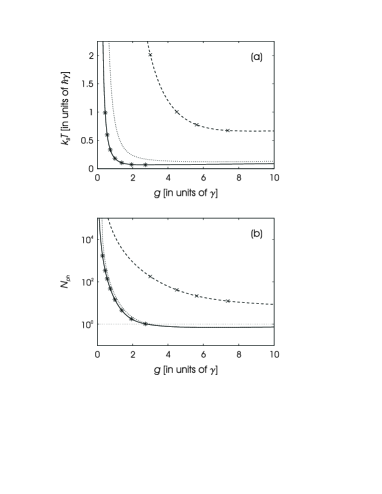
Figure 4: Steady-state temperature (a), and the number of spontaneously scattered photons in a cooling time (b) versus the effective coupling constant $g_{\mbox{\tiny eff}}$. Dashed line corresponds to $\kappa=\gamma$, the solid one to $\kappa=\gamma/10$. The crosses put on the curves indicate the coupling constant corresponding to maximum transverse indices of $2N=0,2,4,8$, …, with starting a single-mode coupling constant of $g=3\gamma$ for the dashed curve of $\kappa=\gamma$, and $g=3\gamma/10$ for the solid curve of $\kappa=\gamma/10$. For this latter the single-mode coupling (maximum index 0) is missing from the plotted range of temperatures.

The rapid drop in temperature obtained when the number of modes included slightly increases is the main benefit we can expect from the use of a multimode cavity. In both cases, $\kappa=\gamma$ and $\kappa=\gamma/10$ sub-Doppler temperatures can be achieved with a small number of modes involved. Note also that the curves converge fast, indicating the existence of a well-defined temperature insensitive to the divergence of the effective coupling constant $g_{\mbox{\tiny eff}}$ with increasing number of modes.

In addition to the induced atomic dipole moment, the driving field yields a small, but not completely negligible atomic excitation. Hence, spontaneous photon scattering occurs with a rate of $2\gamma\langle\sigma^{\dagger}\sigma\rangle$. It is an important quantity how many photons are scattered in this way during the characteristic time of cooling which is $(2\beta)^{-1}$ in our case. The principal goal is to restrict this number below one which implies that the scheme can be extended for cooling particles without closed pumping cycle. The Fig. 4b shows that the number of spontaneously scattered photons in a cooling time, $N_{\mbox{\tiny ph}}=\gamma\langle\sigma^{\dagger}\sigma\rangle/\beta$, can decrease below the limit of one photon for large enough $g_{\mbox{\tiny eff}}$, corresponding to about $N=64$.

Both quantities plotted in Fig. 4 are independent of the pumping strength. The cooling time itself depends on it. However, without specifing a driving field intensity, one can deduce numerical values of the cooling time from the Fig. 4b, provided the saturation is kept fixed. For example, at a saturation $\langle\sigma^{\dagger}\sigma\rangle\approx 0.1$, and for Rb with $\gamma=20/\mu$s, the cooling time is $N_{\mbox{\tiny ph}}/4$ in units of $\mu$s.

The result exhibited in Fig. 4 suggests that smaller $\kappa$ provides better performances in terms of temperature, cooling time. On the other hand, as it was pointed out in vuletic01 ; horak01 , the velocity capture range is limited by $kv<\kappa$.

Finally, let us return to the problem already addressed in the last section. Fig. 4 presents an additional curve (dotted line) that corresponds to the same parameter setting as the one belonging to the solid line ($\kappa=\gamma/10$), however, the single-mode cavity field is being pumped instead of the atom. Whatever component is driven externally, the pumping field, by construction of the detunings, is resonant with the lower dressed state at an antinode, and this analogy makes the comparison justified. It is apparent that the temperature in the atom-driven case is lower. The curve belonging to the cavity-driven case for $\kappa=\gamma$ does not even fit in the plotted range, the difference with respect to the dashed line is much larger. Although a simple transformation connects the results of the atom- and cavity-driven cases, as this example illustrates it, a significant physical difference can occur. The origin is that the detunings were the same, $\Delta_{A}$ is large and $\Delta_{C}$ is small, which breaks the symmetry between the two systems based on the interchange of the above detunings.

V.2 Beyond the effective mode approach

The effective mode approach could be used in the previous analysis because all the relevant modes closely overlapped in the region of interest, i. e., around the cavity center. Accordingly, the system is reminiscent of a single-mode one with enlarged coupling constant $g_{\mbox{\tiny eff}}$. By contrast, when one moves away from the center, but still on the axis, the cosine-like mode functions with varying wavenumbers undergo a dephasing. One immediate consequence is that the friction force, proportional with the gradient of the mode function, does not vanish in any point. Furthermore, on inspecting the general solutions (18) and (19), one can notice that the friction coefficient $\beta$ is proportional to the square of the sum $\partial_{z}\sum g_{k}^{2}(z)$, while the diffusion coefficient, for $\Delta_{C}\cong 0$ contains only the sum $\sum(\partial_{z}g_{k})^{2}$. Although the determinant $|D|^{2}$ appears also on different powers in the denominator, it is clear that for certain parameter settings the two coefficients can scale in a different way with the number of modes. This gives rise to the possibility to get an interferometric enhancement of the cooling by a collective effect of the modes and leads us to conjecture that the steady-state temperature can be lower in other positions than the cavity center.

To check this expectation, we calculated the temperature as a function of the position in the cavity by using the mode functions $\cos\{(kz-(2m+2n+1)\mbox{atan}(z/z_{0})\}$ with transverse indices $n,m=0,1,N$, where the Guoy-phase term is responsible for shifting the modes out of phase. The length scale of the dephasing can be estimated by $z/l_{\mbox{\tiny cav}}\sim\pi/4(2N+1)$, i. e., at this distance from the center the Guoy-phase shift is about $\pi/2$. For each position, (i) we perform again the averaging of the diffusion and friction coefficients over a wavelength, and (ii) we redefine the detunings $\Delta_{A}$, $\Delta_{C}$ such that the lower-dressed state corresponding to the local coupling constant be resonantly pumped at antinodes. The result is plotted in figure 5.

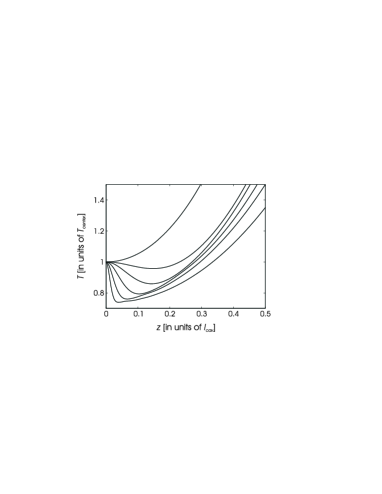
Figure 5: Steady-state temperature as a function of the position in the cavity for $\kappa=\gamma/10$, $g=3\gamma/10$. The temperature in the center is used as a unit, therefore purely the competitive effects of the dephasing and the decrease of the coupling strength when moving away from the waist can be observed. The curves correspond 0, 2, 4, 8, 16 and 32 as maximum index taken into account.

The temperature initially drops as the atom moves out from the center. The higher indices are taken into account, the faster the initial drop happens, which suggests that the underlying reason is indeed the dephasing of the cosine modes. The estimated length scale shows a good agreement with the numerically obtained results for various maximum indices $2N$. The reduction of about $20\%$ in the temperature can be attributed to a collective, interference-like effect of the multimode field. For large distances from the center, after the dephasing is completed, the temperature grows slowly again, exhibiting the effect of the decreasing coupling constant.

VI Conclusions

The mechanical effects of a high-$Q$ cavity on the center–of–mass motion of a coherently-driven neutral atom have been investigated. We calculated the diffusion coefficient and the friction force from a quantum model adapted to the strong atom-field coupling regime, hence the validity does not depend on any specific relationship of the parameters. The model is analogous to the one described in Refs. horak97 ; hechenblaikner98 , however, we considered the system with the atom being externally pumped instead of the cavity field mode. Surprisingly, this difference leads to important new features in the diffusion and damping process. Lower temperatures can be achieved in the present system. We pointed out that certain cooling mechanisms can be realized only in the good-cavity limit, i.e. $g\gg\kappa,\gamma$, where the dressed-atom dynamics including Rabi oscillations becomes dominant. The corresponding parameter regimes are especially suited to applications, since large atomic detunings (red or blue) are allowed here. Furthermore, we found that drastic improvement in terms of low temperature and small number of spontaneous scattering can be obtanied in a degenerate multimode resonator. As a highlight of this possible benefit, we showed that the number of spontaneously emitted photons from the atom during the cooling time can be reduced to below one, which demonstrates the possibility of cooling molecules optically below the Doppler limit.

- (1) T. W. Mossberg, M. Lewenstein, and D. J. Gauthier, Phys. Rev. Lett. 67, 1723 (1991).
- (2) M. Lewenstein and L. Roso, Phys. Rev. A 47, 3385 (1993).
- (3) J. I. Cirac, M. Lewenstein, and P. Zoller, Phys. Rev. A 51, 1650 (1995).
- (4) V. Vuletić and S. Chu, Phys. Rev. Lett. 84, 3787 (1999).
- (5) V. Vuletić, H. W. Chan, and A. T. Black, Phys. Rev. A 64, 033405 (2001).
- (6) P. Horak, G. Hechenblaikner, K. M. Gheri, H. Stecher, and H. Ritsch, Phys. Rev. Lett. 79, 4974 (1997).
- (7) G. Hechenblaikner, M. Gangl, P. Horak, and H. Ritsch, Phys. Rev. A 58, 3030 (1998).
- (8) P. W. H. Pinkse, T. Fischer, P. Maunz, and G. Rempe, Nature 404, 365 (2000).
- (9) C. J. Hood, T. W. Lynn, A. C. Doherty, A. S. Parkins, and H. J. Kimble, Science 287, 1447 (2000).
- (10) P. Horak and H. Ritsch, Phys. Rev. A 64, 033422 (2001)
- (11) C. Cohen-Tannoudji, in “Fundamental Systems in Quantum Optics”, Proceedings of the Les Houches Summer School 1990, Session LIII, edited by J. Dalibard, J.-M. Raimond, and J. Zinn-Justin (Elsevier Science, Amsterdam, 1992).
- (12) P. Horak, H. Ritsch, T. Fischer, P. Maunz, T. Puppe, P. W. H. Pinkse, and G. Rempe, Phys. Rev. Lett. 88, 043601 (2002).
- (13) P. Domokos, P. Horak, and H. Ritsch, J. Phys. B: At. Mol. Opt. Phys. 34 187 (2001).
- (14) T. Fischer, P. Maunz, T. Puppe, P. W. H. Pinkse, and G. Rempe, New Journal of Physics 3, 11.1-11.20 (2001).