Asymptotic Relative Entropy of Entanglement for Orthogonally Invariant States

Abstract

For a special class of bipartite states we calculate explicitly the asymptotic relative entropy of entanglement $E_{R}^{\infty}$ with respect to states having a positive partial transpose (PPT). This quantity is an upper bound to distillable entanglement. The states considered are invariant under rotations of the form $O\otimes O$, where $O$ is any orthogonal matrix. We show that in this case $E_{R}^{\infty}$ is equal to another upper bound on distillable entanglement, constructed by Rains. To perform these calculations, we have introduced a number of new results that are interesting in their own right: (i) the Rains bound is convex and continuous; (ii) under some weak assumption, the Rains bound is an upper bound to $E_{R}^{\infty}$; (iii) for states for which the relative entropy of entanglement $E_{R}$ is additive, the Rains bound is equal to $E_{R}$.

I Introduction

In spite of the impressive recent progress in the theory of entanglement entanglement , many fundamental questions or challenges still remain open. One of these issues is to decide whether a given state is entangled or not. Another question is to find criteria for the distillability of a state, i.e. whether pure state entanglement can be recovered from the original state by means of local operations and classical information exchange.

Since entangled states are a resource in many basic protocols in quantum computation and quantum communication, a need has emerged to quantify entanglement. This leads to more advanced challenges: how much entanglement is needed to create a given state and how much entanglement can be recovered?

Since these questions lead to very high dimensional optimization problems, it is often helpful or even inevitable to restrict oneself to states exhibiting a very high symmetry. The two most common one-parameter families of symmetric states are the so-called ‘Werner’ states Werner89 and the ‘Isotropic’ states, which are related to one another via the partial transposition operation. A larger set of symmetric states, containing these two sets as special cases, are the OO-invariant states, which are the states considered in this paper.

So far it is not known how to calculate distillation rates for arbitrary states, and even for symmetric states this optimization seems to be intractable. One possible way to partially circumvent this problem is to calculate good bounds for the distillation rates. A well-known upper bound for the distillable entanglement is the relative entropy of entanglement relent , which is itself defined as an optimization:

$$E_{R}(\rho)=\inf_{\sigma\in{\cal D}}S(\rho||\sigma).$$

In this formula, $S(\rho||\sigma)=\mathop{\mathrm{missing}}{Tr}\nolimits(\rho\log\rho-\rho\log\sigma)$ is the relative entropy (the quantum mechanical analog of the Kullback-Leibler divergence) and the minimum is taken over all states $\sigma$ in the convex set $\cal D$. The relative entropy between two states is a measure of distinguishability and can intuitively be regarded as a kind of distance measure, although it violates most of the axioms that are required of a distance measure relent . In the originally proposed definition of the relative entropy of entanglement, $\cal D$ is the set of separable states, so that the $E_{R}(\rho)$ expresses the minimal distinguishability between the given state and all possible separable states. When using the $E_{R}$ as an upper bound to distillability, however, it is fruitful to enlarge the set $\cal D$ to the set of states with positive partial transpose (the PPT states) Rains_Lemma . The corresponding minimal relative entropy, the relative entropy of entanglement with respect to PPT states (REEP), is generally smaller than the (separability) relative entropy of entanglement while it still is an upper bound to distillability; this is so because all PPT states have distillability zero. Hence, the REEP is a sharper bound on the distillability than the separability relent. This enlargement of $\cal D$ has the additional benefit that the set of PPT states is much easier to characterize than the set of separable states, for which no general operational membership criterion exists.

Nevertheless, neither for the REEP nor for the relative entropy of entanglement is there a general solution known of the optimization problem for arbitrary states, not even for the otherwise simple case of two qubits. However, the calculations become tractable when restricting oneself to symmetric states.

Contrary to earlier conjectures, neither REEP nor the relative entropy of entanglement is additive, i.e. $E_{R}(\rho_{1}\otimes\rho_{2})\leq E_{R}(\rho_{1})+E_{R}(\rho_{2})$ is a strict inequality for some states. It is expected, however, that this non-additivity becomes less severe for the asymptotic relative entropy of entanglement with respect to PPT states(AREEP), which is defined as the regularisation

$$E_{R}^{\infty}(\rho)=\lim_{n\rightarrow\infty}\frac{1}{n}E_{R}(\rho^{\otimes n}),$$

and which at the same time provides yet a sharper bound to distillable entanglement.

The calculation of the AREEP has first been done on Werner states ka , showing that the asymptotic value can be a good deal smaller than the single-copy value. Surprisingly, it turns out that on Werner states the AREEP is equal to another upper bound on distillability, the so-called Rains bound Rains_semidef

$$R(\rho)=\inf_{\sigma}S(\rho||\sigma)+\log\mathop{\mathrm{missing}}{Tr}\nolimits|\sigma^{T_{2}}|.$$ (1)

One of the things we will show in this paper is that this equality remains valid over the larger class of OO-invariant states.

To calculate the AREEP on OO-invariant states in a relatively simple way, we will make use of four ingredients:

• First of all, REEP is additive on a large part of the state space. This will be discussed in Sec. II. For this additive region, the calculation of the AREEP is trivial, as the (single-copy) REEP for OO-invariant states has been calculated before.

• We will make use of the convexity of the AREEP (recollected in Sec. III) and of the Rains bound (proven in Sec. IV). In Sec. III we use this convexity to define the “minimal convex extension” of the AREEP from the additive areas to the full state space.

• In Sec. V we will present a close connection between the Rains Bound $R(\rho)$ and the AREEP. We will establish an upper bound to the AREEP that will turn out to be tight on OO-invariant states.

• In Sec. VI.2 we will recall the basic properties of OO-invariant states resulting from their symmetry. It is exactly this symmetry that makes the calculation feasible.

Using these results, we will give a complete calculation of the AREEP of OO-invariant states in Sec. VI and prove that this quantity is equal to the Rains bound for these states. We will summarise the results of the paper in Sec. VII and state a number of open problems.

II Additivity of relative entropy of entanglement

The additivity of the REEP was a folk conjecture, supported by various numerical calculations and analytical case studies. Nevertheless, it turned out to be wrong vollbrecht1 . The misleading numerical result can be explained in hindsight by the fact that, indeed, in great parts of the state space the REEP is perfectly additive; the non-additive regions seem to be negligible in size compared to the whole state space.

The following Lemma of Rains Rains_Lemma can be utilized to pinpoint regions where the REEP is additive.

Lemma 1 (Rains-Additivity)

Let $\rho$ be a state and $\sigma$ a PPT state, such that $E_{R}(\rho)=S(\rho||\sigma)$ and $[\rho,\sigma]=0$. If the condition

$$|(\rho\sigma^{-1})^{T_{2}}|\leq\openone$$ (2)

holds, then the REEP is weakly additive on $\rho$, i.e., $E^{\infty}_{R}(\rho)=E_{R}(\rho)$. If it satisfies the stronger condition

$$0\leq(\rho\sigma^{-1})^{T_{2}}\leq\openone$$ (3)

then REEP is strongly additive, i.e., $E_{R}(\rho\otimes\tau)=E_{R}(\rho)+E_{R}(\tau)$ holds for an arbitrary state $\tau$.

Knowing the optimal $\sigma$ for a given state $\rho$, it is straightforward to check condition (2). Checking the additivity therefore only requires one to calculate the REEP.

III Convexity of the asymptotic relent

By definition, the asymptotic version of a given quantity inherits most of the important properties directly from its single-copy “parent” quantity. One such property, which will turn out to be very helpful to calculate the AREEP, is convexity. The REEP itself is known to be convex, but it is not obvious that quantities of the form $E_{n}(\rho):=E(\rho^{\otimes n})/n$ should be convex functions in $\rho$ too and, in fact, this does not hold in general. Although convexity might not hold for finite $n$, for the REEP it becomes valid again in the asymptotic limit.

Lemma 2

rudolph Let $E$ be a positive, subadditive, convex and tensor-commutative functional on the density matrices of a Hilbert space. Then the asymptotic measure $E^{\infty}(\rho):=\lim_{n\rightarrow\infty}\frac{1}{n}E(\rho^{\otimes n})$ exists and is convex and subadditive.

In the first calculation of the AREEP ka great effort was necessary to construct a lower bound to AREEP. Utilizing the convexity we are now able to do this in a much simpler way. Indeed, for any convex (differentiable) function $f$, a lower bound to $f$ is given by any of its tangent planes

$$f(x)\geq f(y)+\nabla f(y)(x-y).$$

Given an open subset $D$ where the function $f$ is known, we can define the “minimal convex extension” of the function by

$$\bar{f}(x)=\sup_{y\in D}f(y)+\nabla f(y)(x-y).$$

Note that $\bar{f}$ is equal to $f$ on $D$. Furthermore, $\bar{f}$ is smaller or equal than any convex function that equals $f$ on $D$. As a maximum over affine functions it is itself convex.

To make this bound a good candidate for an estimation to the AREEP, we need to know the AREEP on a sufficiently large part of the state space. In fact the AREEP is easy to calculate on PPT states, where it is simply zero. But this is obviously too trivial a result, because this gives a lower bound equal to zero on the whole state space. The next greater set for which we can easily calculate the AREEP is the set of states where $E_{R}^{\infty}$ is additive. A subset of this set can be found using the Lemma of Rains. It will turn out that this subset is large enough to yield a bound that equals $E_{R}^{\infty}$ (at least for OO-invariant states).

IV Convexity and continuity of the Rains bound

Although the function that is to be minimized in Rains’ bound, $S(\rho||\sigma)+\log\mathop{\mathrm{missing}}{Tr}\nolimits|\sigma^{T_{2}}|$, is not convex in $\sigma$ over state space, the minimum itself turns out to be convex in $\rho$. We prove this by first showing that the minimization problem in the calculation of the Rains bound can be converted to a convex problem.

To begin with, we can add a third term to the function to be minimized, namely $-\log\mathop{\mathrm{missing}}{Tr}\nolimits[\sigma]$, because this term is zero anyway. Secondly, we can enlarge the set over which one has to minimize from the set of normalized states to the set ${\cal S}=\{s\geq 0,\mathop{\mathrm{missing}}{Tr}\nolimits[s]\leq 1\}$. This is so because the sum of the first two terms is independent of $\mathop{\mathrm{missing}}{Tr}\nolimits[\sigma]$ and the third one monotonously decreases with $\mathop{\mathrm{missing}}{Tr}\nolimits[\sigma]$; hence, the minimal value must be found on the boundary of $\cal S$ corresponding with $\mathop{\mathrm{missing}}{Tr}\nolimits[\sigma]=1$ and is, therefore, equal to the original minimum. The second and third term can now be absorbed in the first term: $S(\rho||\sigma)+\log\mathop{\mathrm{missing}}{Tr}\nolimits|\sigma^{T_{2}}|-\log\mathop{\mathrm{missing}}{Tr}\nolimits\sigma=S(\rho||\sigma(\mathop{\mathrm{missing}}{Tr}\nolimits\sigma/\mathop{\mathrm{missing}}{Tr}\nolimits|\sigma^{T_{2}}|))$. Defining

$$\tau=\sigma(\mathop{\mathrm{missing}}{Tr}\nolimits\sigma/\mathop{\mathrm{missing}}{Tr}\nolimits|\sigma^{T_{2}}|),$$

it is easy to check that $\sigma\in{\cal S}$ if and only if $\tau\in{\cal T}=\{t\geq 0,\mathop{\mathrm{missing}}{Tr}\nolimits|t^{T_{2}}|\leq 1\}$. Hence, the calculation of the Rains bound has been transformed to the minimization problem

$$R(\rho)=\min_{\tau\in{\cal T}}S(\rho||\tau).$$

The importance of this transformation stems from the fact that the resulting optimization problem is a so-called convex optimization problem: the function to be minimized is now convex in $\tau$, while the set over which the minimization is performed is still convex. The latter statement follows directly from the convexity of the negativity. Indeed, if $\tau_{1}$ and $\tau_{2}$ are in $\cal T$, then they are positive and have negativity $\leq 1$. Hence, any convex combination of $\tau_{1}$ and $\tau_{2}$ is positive and has negativity $\leq 1$ as well, and, therefore, belongs to the set $\cal T$.

It is now easy to prove continuity and convexity of the Rains bound itself. Continuity follows by noting that the proof of continuity of the quantity $\inf_{\sigma\in\cal D}S(\rho||\sigma)$ in continuity , where $\cal D$ is a compact convex set of normalized states containing the maximally mixed state, does actually not depend on the trace of the various $\sigma$ in $\cal D$. Hence, the theorem is also true for convex sets $\cal D$ containing non-normalized states, and, specifically, for the set $\cal T$.

Convexity is also proven in the standard way, as has been done for $E_{R}$ relent . The standard proof again depends only on the convexity of the feasible set and not on the normalization of the states it contains.

In this way we have proven:

Lemma 3

The calculation of the Rains bound can be reformulated as a convex minimization problem:

$$R(\rho)=\min\{S(\rho||\tau):\tau\geq 0,\mathop{\mathrm{missing}}{Tr}\nolimits|\tau^{T_{2}}|\leq 1\}.$$

The Rains bound itself is a continuous and convex function of $\rho$.

V Relation between Rains’ bound and the AREEP

The results of the calculation of the AREEP on Werner states suggests rains_private that this quantity might be connected with the quantity (1) defined by Rains, and, moreover, that there are connections between the minimizing $\sigma$ in Rains’ formula and the asymptotic PPT state $\sigma$ appearing in $E_{R}^{\infty}$. Indeed, it turns out that one can give a simple relation between these two quantities, if we require as an additional restriction that $\sigma$ in (1) satisfies $|\sigma^{T_{2}}|^{T_{2}}\geq 0$. If the restriction does not hold the Lemma might still be true, but we have not been able to prove this.

Lemma 4

An upper bound for the AREEP is given by

$$R^{\prime}(\rho) := \inf^{*}_{\sigma}S(\rho||\sigma)+\log(\mathop{\mathrm{missing}}{Tr}\nolimits|\sigma^{T_{2}}|)$$ (4)

$$\geq E^{\infty}_{R}(\rho),$$

where the asterisk means that the infimum is to be taken over all states $\sigma$ satisfying

$$|\sigma^{T_{2}}|^{T_{2}}\geq 0.$$ (5)

We will refer to the quantity $R^{\prime}(\rho)$ as the modified Rains bound. The set of states satisfying condition (5) is easily seen to be convex, so that the modified Rains bound is also continuous and convex.

Proof: It can easily be seen that the Lemma is valid if we restrict $\sigma$ to be a PPT state, since then the second term in (4) vanishes and we get the trivial inequality $E^{\infty}_{R}(\rho)\leq E_{R}(\rho)$. This means that we can restrict ourselves to the case where $\sigma$ is a non-PPT state, i.e. $\mathop{\mathrm{missing}}{Tr}\nolimits|\sigma^{T_{2}}|>1$.

Let $\sigma$ be an arbitrary non-PPT state such that $\bar{\sigma}:=|\sigma^{T_{2}}|^{T_{2}}\geq 0$, then

$$\sigma_{n}=\frac{\sigma^{\otimes n}+\bar{\sigma}^{\otimes n}}{1+(\mathop{\mathrm{missing}}{Tr}\nolimits{\bar{\sigma}})^{n}}$$

is a PPT-state. Taking this PPT state as a trial state in the optimization for the AREEP, we get

$$E_{R}(\rho^{\otimes n}) \leq S(\rho^{\otimes n}||\sigma_{n})=S\left(\rho^{\otimes n}||\frac{\sigma^{\otimes n}+\bar{\sigma}^{\otimes n}}{1+(\mathop{\mathrm{missing}}{Tr}\nolimits{\bar{\sigma}})^{n}}\right)$$

$$\leq S\left(\rho^{\otimes n}||\frac{\sigma^{\otimes n}}{1+(\mathop{\mathrm{missing}}{Tr}\nolimits{\bar{\sigma}})^{n}}\right)$$

$$= nS(\rho||\sigma)+\log(1+(\mathop{\mathrm{missing}}{Tr}\nolimits\bar{\sigma})^{n}).$$

In (V) we have used the fact that the relative entropy is operator anti-monotone in its second argument (Corollary 5.12 of Ohya ), i.e. $S(\rho||\sigma+\tau)\leq S(\rho||\sigma)$ for positive $\tau$. Taking the limit $n\rightarrow\infty$ and using $\mathop{\mathrm{missing}}{Tr}\nolimits\bar{\sigma}>1$ we get

$$E^{\infty}_{R}(\rho) = \lim_{n\rightarrow\infty}\frac{1}{n}E_{R}(\rho^{\otimes n})$$ (7)

$$\leq \lim_{n\rightarrow\infty}S(\rho||\sigma)+\frac{\log(1+(\mathop{\mathrm{missing}}{Tr}\nolimits\bar{\sigma})^{n})}{n}$$

$$= S(\rho||\sigma)+\log\mathop{\mathrm{missing}}{Tr}\nolimits\bar{\sigma}.$$

In order to get the best bound, we take the minimum over all feasible states $\sigma$ in equation (7), giving

$$E^{\infty}_{R}(\rho)\leq\inf^{*}_{\sigma}S(\rho||\sigma)+\log\mathop{\mathrm{missing}}{Tr}\nolimits|\sigma|^{T_{2}}$$

where the infimum is taken over all states $\sigma$ satisfying $|\sigma^{T_{2}}|^{T_{2}}\geq 0$. $\square$

It is easy to see that for PPT states $\sigma$, $|\sigma^{T_{2}}|^{T_{2}}\geq 0$. Hence, the feasible set in the minimization of $E_{R}$ is a subset of the one for $R^{\prime}$, which is again a subset of the one for $R$. Therefore, we have the inequalities

$$R(\rho)\leq R^{\prime}(\rho)\leq E_{R}(\rho).$$

We also have the following Theorem:

Theorem 5

For $E_{R}$-additive states $\rho$ (i.e. $E_{R}(\rho)=E_{R}^{\infty}(\rho)$), the Rains bound is equal to the AREEP and is additive.

Proof: We have, in general, $R^{\prime}(\rho)\leq E_{R}(\rho)$. On the other hand, for additive states $E_{R}(\rho)=E_{R}^{\infty}(\rho)$, and $E_{R}^{\infty}(\rho)\leq R^{\prime}(\rho)$ by the Lemma 4. Therefore, $R^{\prime}(\rho)=E_{R}(\rho)=E_{R}^{\infty}(\rho)$ for all additive $\rho$. This also implies that the PPT state $\sigma$ that is optimal for $E_{R}$ is also optimal for $R^{\prime}$.

To show that $R$ is also equal to $E_{R}$, we need to show that this $\sigma$ is optimal for $R$ as well. We use the reformulation of the Rains bound as a convex minimization problem $R(\rho)=\min_{\tau}\{S(\rho||\tau):\mathop{\mathrm{missing}}{Tr}\nolimits|\tau^{T_{2}}|\leq 1\}$. For the modified Rains bound, we have the additional restriction on the feasible set that $|\tau^{T_{2}}|^{T_{2}}\geq 0$. For clarity, let us write $\tau$ for the optimal $\tau$ for $R$ and $\tau^{\prime}$ for the optimal one for $R^{\prime}$. We have to show that $\tau=\tau^{\prime}$, i.e. that $\tau$ is in the set for which $|\tau^{T_{2}}|^{T_{2}}\geq 0$.

Suppose $\tau$ were outside this set, then, following a general property of convex optimization problems, $\tau^{\prime}$ would have to be on the boundary of the set, i.e. $|\tau^{\prime T_{2}}|^{T_{2}}$ would have to be positive and rank-deficient. On the other hand, we already showed that the optimal $\sigma^{\prime}$ for $R^{\prime}$ for additive $\rho$ must be PPT, so that $\tau^{\prime}=\sigma^{\prime}$ and $|\sigma^{\prime T_{2}}|^{T_{2}}=\sigma^{\prime}$. Therefore, the rank-deficiency of $|\tau^{\prime T_{2}}|^{T_{2}}$ implies that $\sigma^{\prime}$ itself should be rank-deficient. However, if $\rho$ is not itself rank-deficient, then this cannot be, because $\sigma^{\prime}$ appears as second argument in the relative entropy and would then give an infinite relative entropy, contrary to the statement that $\sigma^{\prime}$ actually minimises it. This proves that $R^{\prime}(\rho)=R(\rho)$ for full-rank, additive $\rho$. By continuity of the Rains bound this must then also hold for rank-deficient $\rho$.

Additivity of $R$ for $E_{R}$-additive states follows by regularising both sides of the equality $R(\rho)=E_{R}^{\infty}(\rho)$, and noting that the right-hand side does not change. $\square$

We have introduced the operation $\sigma\mapsto|\sigma^{T_{2}}|^{T_{2}}$ as a mathematical tool, and we doubt whether it has any real physical significance (as was the case for the partial transpose). Nevertheless, its usefulness is apparent from the above Lemma. A natural question to ask is whether there really are states $\sigma$ for which $|\sigma^{T_{2}}|^{T_{2}}$ is not positive. We call states like this binegative states. If they would not exist, then the modified Rains bound would just be equal to the original Rains bound. We have performed numerical investigations that have shown that, indeed, binegative states exist, provided the dimensions of the system are higher than $2\times 2$. For $2\times 2$ systems, extensive calculations failed to produce binegative states, which suggests they might not exist in such systems. For higher dimensions, binegative states have been produced, and they always appear to be located close to the boundary of state space, i.e. have a smallest eigenvalue which is very small. In the present setting, this is good news, because it implies that the modified Rains bound will typically be close to the original Rains bound.

As one of the few exact results on the existence of binegative states, we have been able to prove that pure states are never binegative:

Lemma 6

For any pure state $\psi$, $\big{|}|\psi\rangle\!\langle\psi|^{T_{2}}\big{|}^{T_{2}}\geq 0$.

Proof: Let $\psi$ have a Schmidt decomposition $\psi=\sum_{i}\lambda_{i}u_{i}\otimes v_{i}$, then $|\psi\rangle\!\langle\psi|^{T_{2}}=\sum_{i,j}\lambda_{i}\lambda_{j}|u_{i}\rangle\!\langle u_{j}|\otimes|v_{i}\rangle\!\langle v_{j}|^{T}$ and, exploiting the orthogonality of the vectors $u_{i}$ and of the vectors $v_{j}$,

$$\big{|}|\psi\rangle\!\langle\psi|^{T_{2}}\big{|} = \big{(}\sum_{i,j,k,l}\lambda_{i}\lambda_{j}\lambda_{k}\lambda_{l}|u_{i}\rangle\!\langle u_{j}||u_{k}\rangle\!\langle u_{l}|\otimes$$

$$(|v_{k}\rangle\!\langle v_{l}||v_{i}\rangle\!\langle v_{j}|)^{T}\big{)}^{1/2}$$

$$= \big{(}\sum_{i,j}(\lambda_{i}\lambda_{j})^{2}|u_{i}\rangle\!\langle u_{i}|\otimes|v_{j}\rangle\!\langle v_{j}|^{T}\big{)}^{1/2},$$

since only the terms with $i=l$ and $j=k$ survive. Again by orthogonality, taking the square root amounts to removing the square on the factor $(\lambda_{i}\lambda_{j})^{2}$. Now, one clearly sees that the resulting expression corresponds to a product state; hence, the partial transpose is still a state, which proves that $\psi$ is not binegative. $\square$

In Section VI.2 we will show that no OO-invariant state is binegative either. We will see that condition (5) will be fulfilled for the states we are considering in this paper. Therefore, we will henceforth make no distinction anymore between $R$ and $R^{\prime}$.

VI OO-Invariant states

We will now apply the tools obtained in the previous sections to the complete calculation of the AREEP of OO-invariant states.

VI.1 Calculating the AREP on Werner states

To illustrate how the calculation of the AREEP on OO-invariant states will proceed, we apply the method first on Werner states, reproducing the results of ka .

Werner states can be written as

$$\rho(p)=p\frac{P_{-}}{r_{-}}+(1-p)\frac{P_{+}}{r_{+}},$$

where $P_{+}(P_{-})$ denotes the normalized projection onto the symmetric (antisymmetric) subspace of dimension $r_{\pm}=\frac{d^{2}\pm d}{2}$ and $p$ is a real parameter ranging from $0$ to $1$.

First of all, we need to know $E_{R}$ on these states. All states with $p\leq\frac{1}{2}$ are PPT and, therefore, have both $E_{R}$ and $E_{R}^{\infty}$ equal to zero. For all non-PPT Werner states $p>\frac{1}{2}$, the minimizing PPT-state is the state with $p=\frac{1}{2}$. Knowing this state, we can easily write down the REEP for all Werner states. To calculate the AREEP we use the three steps introduced in the previous three Sections.

In the first step we use the lemma of Rains and check the additivity condition (2). An easy and straightforward calculation leads to the result that all Werner states satisfying $p\leq\frac{1}{2}+\frac{1}{d}$ are additive and, therefore, have $E_{R}$ equal to $E_{R}^{\infty}$.

In the second step we calculate the Rains bound for Werner states. Due to the high symmetry this is an easy task, already done by Rains Rains_semidef . In fact, we do not need to compute the Rains bound for all states. For our purposes, we will only need the Rains bound for $p=1$.

In the last step we calculate the tangent to the REEP in the point $p=\frac{1}{2}+\frac{1}{d}$, which gives us the minimal convex extension for all states with $p>\frac{1}{2}+\frac{1}{d}$. It turns out that this minimal extension touches the Rains bound again in the point $p=1$. This is sufficient to prove that the minimal convex extension is equal to $E_{R}^{\infty}$ everywhere. Indeed, by the convexity of $E^{\infty}_{R}$ the tangent yields a lower bound and, furthermore, also implies that the tangent is an upper bound between $p=1$ and $p=\frac{1}{2}+\frac{1}{d}$, because at the end-points it equals $E^{\infty}_{R}$.

In fact, for Werner states, the same result can easily be obtained by the observation that the Rains bound and the minimal convex extension are equal on the whole range of $p$. But for OO-invariant states the task to prove equality of these two quantities will become quite difficult. Fortunately, we can restrict ourselves to prove equality only on the border of the state space as this will be sufficient for the calculation. Equality of the Rains bound and $E_{R}^{\infty}$ on the whole state space will follow automatically from the convexity of both quantities.

We will now turn to the calculation for the OO-invariant states.

VI.2 Using symmetries

The class of states we want to look at commute with all unitaries of the form $O\otimes O$, where $O$ is an orthogonal matrix. These so-called OO-invariant states lie in the commutant $G^{\prime}$ of the group $G=\{O\otimes O\}$. The commutant is spanned by three operators, the identity operator $\openone$, the Flip operator $\mathbb{F}$ defined as the unique operator for which $\mathbb{F}\psi\otimes\phi=\phi\otimes\psi$ for all vectors $\psi$ and $\phi$, and the unnormalized projection on the maximally entangled state $\widehat{\mathbb{F}}=\sum_{ij}|ii\rangle\!\langle jj|=d|\Psi\rangle\!\langle\Psi|$; here, $d$ is the dimension of either subsystem. Every operator contained in this commutant can be written as a linear combination of these three operators. To be a proper state such an operator has to fulfill the two additional constraints of positivity and normalization.

As coordinates parameterizing the OO-invariant states, we choose the expectation values of the three operators $\openone,\mathbb{F}$ and $\widehat{\mathbb{F}}$ in the given state. The expectation value of the identity, $\big{<}\openone\big{>}_{\rho}$, gives us just the normalization, so we are left with the two free parameters $f:=\big{<}\mathbb{F}\big{>}_{\rho}$ and $\hat{f}:=\big{<}\widehat{\mathbb{F}}\big{>}_{\rho}$. For future reference, we collect the basic formulae here for performing calculations in this representation.

The traces of the basis operators are given by

$$\mathop{\mathrm{missing}}{Tr}\nolimits[\openone] = d^{2}$$

$$\mathop{\mathrm{missing}}{Tr}\nolimits[\mathbb{F}] = d$$

$$\mathop{\mathrm{missing}}{Tr}\nolimits[\widehat{\mathbb{F}}] = d.$$

The inner products between them are easily calculated from the relations

$$\mathbb{F}^{2} =$$

$$\mathbb{F}\widehat{\mathbb{F}} = \widehat{\mathbb{F}}\mathbb{F}=\widehat{\mathbb{F}}$$

$$\widehat{\mathbb{F}}^{2} = d\mathbb{F}.$$

From this basis $\{\openone,\mathbb{F},\widehat{\mathbb{F}}\}$, an orthogonal basis of projectors can be constructed. The operator $\mathbb{F}$ is not positive and can be written as $\mathbb{F}=\mathbb{F}_{+}-\mathbb{F}_{-}$; here $\mathbb{F}_{+}$ and $\mathbb{F}_{-}$ denote the positive and negative part of $\mathbb{F}$, respectively, and are defined by the equations $X=X_{+}-X_{-}$, $|X|=X_{+}+X_{-}$ (note that both the positive and negative part are positive by this definition). Since $\mathbb{F}^{2}=\openone$, $\mathbb{F}_{+}+\mathbb{F}_{-}=\openone$, and $\mathbb{F}_{-}=(\openone-\mathbb{F})/2$. Furthermore, as $\mathbb{F}\widehat{\mathbb{F}}=\widehat{\mathbb{F}}$, $\widehat{\mathbb{F}}<\mathbb{F}_{+}$. Therefore, the following operators form an orthogonal set of projectors and add up to the identity:

$$U = \widehat{\mathbb{F}}/d$$

$$V = (\openone-\mathbb{F})/2$$

$$W = (\openone+\mathbb{F})/2-\widehat{\mathbb{F}}/d.$$

The traces of these projectors are

$$\mathop{\mathrm{missing}}{Tr}\nolimits[U] = 1$$

$$\mathop{\mathrm{missing}}{Tr}\nolimits[V] = d(d-1)/2$$

$$\mathop{\mathrm{missing}}{Tr}\nolimits[W] = (d+2)(d-1)/2.$$

The original basis is related to the orthogonal one by

$$= U+V+W$$

$$\mathbb{F} = U-V+W$$

$$\widehat{\mathbb{F}} = dU.$$

For a general OO-invariant $\rho$, we write

$$\rho=a\openone+b\mathbb{F}+c\widehat{\mathbb{F}}.$$

The relation between the coefficients $a$, $b$, $c$ and $f$ and $\hat{f}$ is given by

$$\left[\begin{array}[]{c}1\\ f\\ \hat{f}\end{array}\right]=d\left[\begin{array}[]{ccc}d&1&1\\ 1&d&1\\ 1&1&d\end{array}\right]\left[\begin{array}[]{c}a\\ b\\ c\end{array}\right],$$

and, inversely, by

$$\left[\begin{array}[]{c}a\\ b\\ c\end{array}\right]=\frac{1}{d(d-1)(d+2)}\left[\begin{array}[]{ccc}d+1&-1&-1\\ -1&d+1&-1\\ -1&-1&d+1\end{array}\right]\left[\begin{array}[]{c}1\\ f\\ \hat{f}\end{array}\right].$$

In terms of the orthonormal basis, $\rho$ can be written as

$$\rho=\frac{\hat{f}}{d}U+\frac{1-f}{d(d-1)}V+\frac{d+df-2\hat{f}}{d(d-1)(d+2)}W.$$ (8)

Positivity of $\rho$ thus amounts to the conditions

$$0 \leq \hat{f}$$

$$f \leq 1$$

$$\hat{f} \leq d(1+f)/2.$$

The representation of the partial transpose of $\rho$ is very easy, since $\mathbb{F}$ and $\widehat{\mathbb{F}}$ are just each other’s partial transpose. Hence, the partial transpose of $\rho$ is obtained by swapping $\mathbb{F}$ and $\widehat{\mathbb{F}}$. In the basis $\{\openone,\mathbb{F},\widehat{\mathbb{F}}\}$, taking the partial transpose corresponds, therefore, to interchanging the parameters $f$ and $\hat{f}$. The partial transposes of the projectors $U$, $V$ and $W$ are easily calculated to be

$$U^{T_{2}} = \frac{1}{d}(U-V+W)$$

$$V^{T_{2}} = \frac{1-d}{2}U+\frac{1}{2}V+\frac{1}{2}W$$

$$W^{T_{2}} = \big{(}\frac{1+d}{2}-\frac{1}{d}\big{)}U+\big{(}\frac{1}{2}+\frac{1}{d}\big{)}V+\big{(}\frac{1}{2}-\frac{1}{d}\big{)}W.$$

From these formulae one can see that the set of OO-invariant states constitutes a triangle in the $(f,\hat{f})$ parameter space, as plotted in Figure 1. Taking the partial transpose amounts to taking the mirror image around the line $f=\hat{f}$. Therefore, the set of PPT states are those contained in the grey square $0\leq f,\hat{f}\leq 1$ in Figure 1.

What will make the calculation of the REEP easy for these OO-invariant states is the existence of a ‘twirl’ operation Werner89 , a projection operation $T$ that maps an arbitrary state $\rho$ to an OO-invariant state $T(\rho)$ and that preserves PPT-ness, i.e., that maps every PPT state to an OO-invariant PPT state. Since

$$S(\rho||\sigma)\geq S(T(\rho)||T(\sigma))$$

this guarantees that the minimum relative entropy for an OO-invariant state is attained on another OO-invariant PPT state Rains_Lemma ; vollbrecht1 . Hence, we can reduce the very high-dimensional optimization problem to an optimization in our two-dimensional OO-invariant state space. This optimization has been done vollbrecht1 and the minimizing PPT states are as follows. Let a state $\rho$ be determined by the expectation values $\big{<}\mathbb{F}\big{>}_{\rho}=f$ and $\big{<}\widehat{\mathbb{F}}\big{>}_{\rho}=\hat{f}$. Similarly, let the expectation values in the optimizing PPT state $\sigma$ be given by $\big{<}\mathbb{F}\big{>}_{\sigma}=s$ and $\big{<}\widehat{\mathbb{F}}\big{>}_{\sigma}=\hat{s}$. Then the following table gives the expressions for $s$ and $\hat{s}$, depending on which region the state $\rho$ is in:

Region	$s$	$\hat{s}$
$A$	$\frac{1+(d-1)f-\hat{f}}{d-\hat{f}}$	$1$
$B$	$0$	$\frac{\hat{f}}{1+f}$
$C$	$0$	$1$

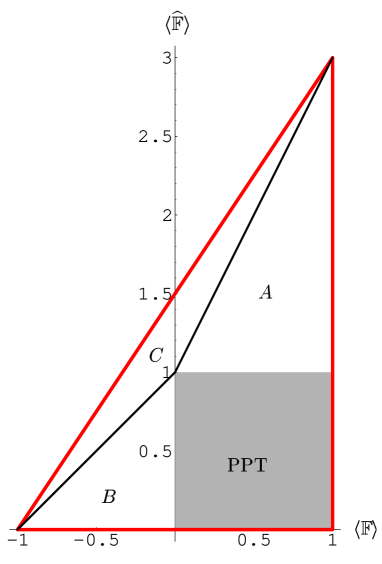
Figure 1: State space of OO-invariant states (case $d=3$). These states are parameterized by the two parameters $f=\langle\mathbb{F}\rangle$ and $\hat{f}=\langle\widehat{\mathbb{F}}\rangle$. The outer triangle represents the values corresponding to states (positivity). The grey area is the set of PPT OO-invariant states. The region of non-PPT states is subdivided further in the three triangular regions labeled $A$, $B$ and $C$. For each of these regions the optimal $\sigma$ appearing in the definition of the REEP is of a different form.

To end this section, we give the formulas for the relative entropy and the negativity of OO-invariant states. Let the states $\rho$ and $\sigma$ be determined by their expectation values $f,\hat{f}$ and $s,\hat{s}$, respectively. Using the state representation (8), in the orthogonal basis $\{U,V,W\}$, the relative entropy of $\rho$ w.r.t. $\sigma$ is given by

$$S(\rho||\sigma) = \frac{\hat{f}}{d}\log\Big{(}\frac{\hat{f}}{\hat{s}}\Big{)}\mathop{\mathrm{missing}}{Tr}\nolimits U+\frac{1-f}{d(d-1)}\log\Big{(}\frac{1-f}{1-s}\Big{)}\mathop{\mathrm{missing}}{Tr}\nolimits V$$ (9)

$$+\frac{d+df-2\hat{f}}{d(d-1)(d+2)}\log\Big{(}\frac{d+df-2\hat{f}}{d+ds-2\hat{s}}\Big{)}\mathop{\mathrm{missing}}{Tr}\nolimits W$$

$$= \frac{\hat{f}}{d}\log\frac{\hat{f}}{\hat{s}}+\frac{1-f}{2}\log\frac{1-f}{1-s}$$

$$+\frac{d+df-2\hat{f}}{2d}\log\frac{d+df-2\hat{f}}{d+ds-2\hat{s}}.$$

Recollecting that taking the partial transpose corresponds to interchanging $s$ and $\hat{s}$, the negativity of $\sigma$ is given by

$$\mathop{\mathrm{missing}}{Tr}\nolimits|\sigma^{T_{2}}| = \left|\frac{s}{d}\right|\mathop{\mathrm{missing}}{Tr}\nolimits U+\left|\frac{1-\hat{s}}{d(d-1)}\right|\mathop{\mathrm{missing}}{Tr}\nolimits V$$ (10)

$$+\left|\frac{d+d\hat{s}-2s}{d(d-1)(d+2)}\right|\mathop{\mathrm{missing}}{Tr}\nolimits W$$

$$= \frac{|s|}{d}+\frac{|1-\hat{s}|}{2}+\frac{|d+d\hat{s}-2s|}{2d}.$$

The positivity condition on $\sigma$ implies that the absolute value sign on the third term is superfluous.

In a similar way, we can show that for any OO-invariant state $\sigma$, the operator $|\sigma^{T_{2}}|^{T_{2}}$ is a state again, as we had promised. Indeed,

$$|\sigma^{T_{2}}|^{T_{2}} = \left|\frac{s}{d}\right|U^{T_{2}}+\left|\frac{1-\hat{s}}{d(d-1)}\right|V^{T_{2}}$$

$$+\left|\frac{d+d\hat{s}-2s}{d(d-1)(d+2)}\right|W^{T_{2}}.$$

An easy but somewhat lengthy calculation shows that this expression can be rewritten in terms of $U$, $V$ and $W$ with positive coefficients.

VI.3 Additive Areas

In the first step we want to identify the areas within the state space triangle where the REEP is additive.

Lemma 7

$E_{R}(\rho)$ is additive for all OO-states satisfying $\big{<}\mathbb{F}\big{>}\geq\frac{-2}{d}$ and $\big{<}\widehat{\mathbb{F}}\big{>}\leq 3-\frac{4}{d}+(d-1)\big{<}\mathbb{F}\big{>}$.

Proof: Utilizing Lemma 1 we only have to check condition (2) for every OO-invariant state $\rho$ and the corresponding optimal PPT-states $\sigma$. In the $\{U,V,W\}$-basis, $\rho\sigma^{-1}$ is directly given by

$$\rho\sigma^{-1}=uU+vV+wW,$$

with

$$u = \frac{\hat{f}}{\hat{s}}$$

$$v = \frac{1-f}{1-s}$$

$$w = \frac{d+df-2\hat{f}}{d+ds-2\hat{s}}.$$

In order to perform the partial transpose, we replace $U,V,W$ by their partial transposes and express them in the original $U,V,W$ again. This yields

$$(\rho\sigma^{-1})^{T_{2}}=(a+bd+c)U+(a-c)V+(a+c)W,$$

with

$$a=\frac{w+v}{2},\,\,b=\frac{w-v}{2},\,\,c=\frac{u-w}{d}.$$

Condition (2) is then satisfied if and only if $|a+c+bd|$, $|a+c|$ and $|a-c|$ are all $\leq 1$. For $s$ and $\hat{s}$ we have to insert the values of the optimal PPT state $\sigma$, obtained at the end of the previous section.

After a tedious calculation, we get 6 conditions an additive state has to satisfy for each of the three regions $A$, $B$ and $C$ of Figure 1. Fortunately, only two of this total of 18 conditions can be violated by expectation values belonging to normalized positive states. In the $A$ region all states are additive, in region $B$ we must have $f\geq-2/d$, and in region $C$ the condition is $\hat{f}\leq 3-4/d+(d-1)f$. These conditions give us the border between the additive and non additive areas. $\square$

The additive area for OO-states is plotted in dark grey in Figure 2 for the dimension $d=3$. States in the light grey area fulfill the condition of strong additivity.

For later use, we have marked some points in the state space that will become important in the further calculation of the AREEP. The two additivity conditions of the Lemma correspond to the boundary line segments CD and BC, respectively.

Point	$\big{<}\mathbb{F}\big{>}$	$\big{<}\widehat{\mathbb{F}}\big{>}$
A	$-1$	$0$
B	$\frac{d-4}{d}$	$d-2$
C	$\frac{-2}{d}$	$\frac{d-2}{d}$
D	$\frac{-2}{d}$	0
E	$0$	$1$
X	$\frac{4-6d+d^{2}}{d(d+2)-4}$	$\frac{d^{2}(d-2)}{d(d+2)-4}$
Y	$\frac{-d^{2}}{d(d+2)-4}$	$\frac{d(d-2)}{d(d+2)-4}$

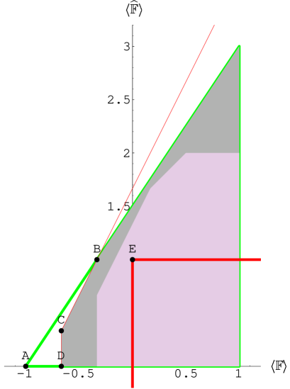
Figure 2: Additive areas for OO-invariant states (case $d=3$). The state space has been subdivided in three regions. According to Rains’ Lemma, the states in the light-grey region are strongly additive and those in the dark-grey region are weakly additive. The region of additivity is delineated by the line segments BC and CD. The points A, B, C, D and E are defined in the text.

VI.4 Rains upper bound

In the second step we want to calculate the Rains bound (4) on the OO-invariant state space. All OO-invariant states satisfy $|\sigma^{T_{2}}|^{T_{2}}\geq 0$, and we therefore restrict the optimization to OO-invariant states $\sigma$. Since we want to use the Rains bound as an upper bound, we need not to know that our so restricted $\sigma$ is really the optimal one. But due to the high symmetry of the OO-states it can easily be shown that the optimum over all possible states $\sigma$ is attained on OO-states anyway.

For additive states we have noted already that $E_{R}(\rho)=E_{R}^{\infty}(\rho)=R(\rho)$ so that calculating the REEP directly gives the Rains bound. To calculate the Rains bound in the non-additive region ABCD, we have to perform the minimization explicitly. Let the states $\rho$ and $\sigma$ be determined by their expectation values $f,\hat{f}$ and $s,\hat{s}$, respectively. Using the formula for the relative entropy of $\rho$ (9) w.r.t. the optimal $\sigma$ for the REEP (see the Table in Section VI.2) yields the Rains Bound for additive states.

For non-additive states we have to include the negativity of $\sigma$, given by (10):

$$\mathop{\mathrm{missing}}{Tr}\nolimits|\sigma^{T_{2}}|=\frac{|s|}{d}+\frac{|1-\hat{s}|}{2}+\frac{d+d\hat{s}-2s}{2d}.$$

As we will only use the above formulae for $\rho$ in the non-additive region ABCD, it is immediately clear from Figure 2 that the optimal $\sigma$ will have negative $s$. We can, therefore, simplify the formula for the negativity to

$$\mathop{\mathrm{missing}}{Tr}\nolimits|\sigma^{T_{2}}| = \frac{-s}{d}+\frac{|1-\hat{s}|}{2}+\frac{d+d\hat{s}-2s}{2d}$$

$$= \max(1,\hat{s})-\frac{2s}{d}.$$

Because of the ‘max’ function appearing in this formula, we have to consider two cases for $\sigma$ and, in the end, choose the solution that gives the smallest value for the Rains bound.

Consider first the case $\hat{s}>1$; then the negativity equals $\hat{s}-2s/d$ and we have to minimize

$$\log\frac{d\hat{s}-2s}{d}+\frac{1}{2d}\Big{[}2\hat{f}\log\frac{\hat{f}}{\hat{s}}+(d-df)\log\frac{f-1}{s-1}$$

$$+(d+df-2\hat{f})\log\frac{d+df-2\hat{f}}{d+ds-2\hat{s}}\Big{]}$$

over $s$ and $\hat{s}$. This function has a single stationary point given by

$$s = \frac{d^{2}-d\hat{f}-2}{(d^{2}-2)f-d\hat{f}}$$

$$\hat{s} = \frac{-2\hat{f}}{(d^{2}-2)f-d\hat{f}}.$$

However, the minimum we are looking for is a constrained one: the parameters $s$ and $\hat{s}$ must be expectation values of positive $\sigma$. On inspection, the positivity conditions are never satisfied in the stationary point for any choice of $f,\hat{f}$ corresponding to a positive $\rho$. Therefore, the stationary point is outside the feasible set (the state triangle) and the constrained minimum will be found on the boundary of the feasible set. This mere fact already rules out the present case $\hat{s}>1$, because we know that the optimal $\sigma$ must be closer to the set of PPT states than $\rho$ itself, in the sense that $\sigma$ should have lower negativity than $\rho$. Indeed, setting $\sigma=\rho$ (which is certainly not optimal) in the Rains bound yields a lower value than one would get for any $\sigma$ with a larger negativity than $\rho$.

We can, therefore, restrict ourselves to the case $\hat{s}\leq 1$. As the negativity is then $1-2s/d$, the function to be minimized is

$$\log\frac{d-2s}{d}+\frac{1}{2d}\Big{[}2\hat{f}\log\frac{\hat{f}}{\hat{s}}+(d-df)\log\frac{f-1}{s-1}$$

$$+(d+df-2\hat{f})\log\frac{d+df-2\hat{f}}{d+ds-2\hat{s}}\Big{]}.$$ (11)

The stationary point is

$$s = \frac{2+df}{d+2f}$$ (12)

$$\hat{s} = \frac{(2+d)\hat{f}}{d+2f}.$$ (13)

Again, $s$ and $\hat{s}$ must be expectation values of positive $\sigma$ and we must have that $\hat{s}\leq 1$. It turns out that the positivity conditions are always fulfilled. The condition $\hat{s}\leq 1$, on the other hand, is only satisfied for states $\rho$ on or below the line going through points C and Y. Therefore, the stationary point is the constrained minimum only for states $\rho$ in the quadrangle AYCD. This leads to the solution for AYCD:

$$R_{AYCD}(\rho) = \frac{1}{2}\big{(}(1+f)\log(d-2)-2\log d$$ (14)

$$-(f-1)\log(d+2)\big{)},$$

which now only depends on the Flip expectation value $f$ and is an affine function of $f$.

For states $\rho$ in the remaining triangle CYB, the stationary point is outside the feasible set, so that the constrained minimum will lie on the line $\hat{s}=1$. Minimization of (11) over $s$, while fixing $\hat{s}=1$, yields a quite cumbersome looking formula. For later use, however, we will only need to know the resulting Rains bound on the line segment YB. The solution consists of two cases, corresponding to either solution of a quadratic equation. The end result is that, for the states on the segment YX, the Rains bound is given by

$$R_{YX}(\rho) = \frac{1+f}{2}\log d(1+f)$$ (15)

$$+\frac{1-f}{2}\log\frac{d(1-f)}{d-1}$$

$$+\log\frac{d(d+2)-4}{d^{2}}-\log 2.$$

For the states on the segment XB the bound is given by

$$R_{XB}(\rho)=\frac{1+f}{2}\log(d-2)+\frac{f-1}{2}\log\frac{d}{4}.$$ (16)

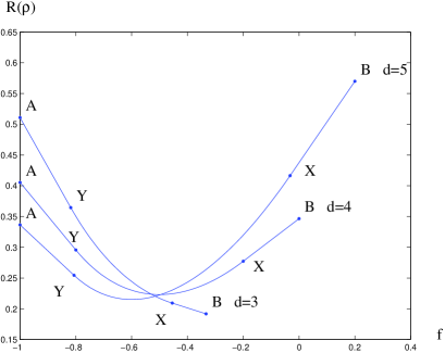
Figure 3: Rains bound on the line segment AB (see Figure 2) in terms of the parameter $f$, for three different values of $d=3,4,5$. The bound consists here of a linear part (segment AY, eq. 14), a curvilinear part (segment YX, eq. 15) and again a linear part (segment XB, eq. 16).

Figure 3 shows the Rains bound along the line segment AB, for several dimensions $d=3,4,5$.

VI.5 Minimal convex extension

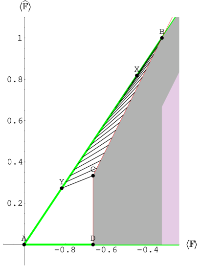
Figure 4: A close-up of the non-additive OO-invariant states in Figure 2, for the purpose of calculating the minimal convex extension to the AREEP. In region AYCD, the minimal convex extension only depends, affinely, on $f$ (eq. 17). In region BCY, the minimal convex extension is affine along the lines depicted here (given by eq. 18).

In this third and final step we calculate the minimal convex extension of the additive area. This will turn out to be more complicated than in the Werner states example. We will look at straight lines, each connecting one point on the additivity border with one, well-chosen point on the line segment AB.

The simplest case is the part of the additivity border consisting of the line segment CD, because this line lies completely in the ‘Werner’ region, region $B$ in Figure 1, where, according to (14), the REEP only depends on the Flip expectation value $f$. So, here, the two-dimensional problem is reduced to a one-dimensional one. The REEP in the Werner triangle is given by

$$E_{R}(f)=\log 2+\frac{(1+f)}{2}\log{\frac{1+f}{2}}+\frac{(1-f)}{2}\log{\frac{1-f}{2}}.$$

As lower bound for the AREEP we get

$$E_{R}^{\infty}(f,\hat{f}) \geq E_{R}(-2/d)+(f+2/d)\frac{\partial E_{R}(f)}{\partial f}\big{|}_{f=-2/d}$$ (17)

$$= \frac{1}{2}(1+f)\log\frac{d-2}{d+2}+\log\frac{2+d}{d},$$

which happens to be identical to the Rains bound (14) in the whole region AYCD. So the upper and lower bound equal each other within this region and, hence, $E_{R}^{\infty}$ is equal to the Rains bound in AYCD.

The situation for the remaining triangle YCB is somewhat more complicated. To calculate $E_{R}^{\infty}$ we consider a set of straight lines connecting points on the line segment BC with points on the segment XY and given by

$$\hat{f}=-pf+\frac{p(d^{2}-2+(d-2)p)}{2+d(p-2)-2p}.$$ (18)

These lines are parameterized by $p$, which runs from $\frac{-2}{d+2}$ to $\frac{-d}{2}$. Recall that the line XY is given by $\hat{f}=(1+f)d/2$ and BC by $\hat{f}=3-4/d+(d-1)f$.

On the line segment XY, the Rains bound is given by (15). On the segment BC, and in fact to the right of it as well, the Rains bound is equal to $E_{R}=E_{R}^{\infty}$ and is given by (9) with $s=0$ and $\hat{s}=1$ (region $C$ of Figure 1). Moreover, this formula holds for all points on the lines (18) within the additivity region, allowing for the calculation of the derivative of the Rains bound along the lines (18). Doing this in the points on the additivity border BC yields the result that, for every line (18), the tangent to the Rains bound at the start point (on segment BC) touches the Rains bound again at the end point (segment XY). By convexity of $E_{R}^{\infty}$ and of the Rains bound, and by the fact that the Rains bound is an upper bound on $E_{R}^{\infty}$ and the tangent a lower bound, it follows that both $E_{R}^{\infty}$ and the Rains bound must coincide with this tangent and, hence, be affine along each of the lines (18). We conclude that $E_{R}^{\infty}$ is equal to the Rains bound also in the remaining region YCB.

VI.6 Summary of results

We finalise the calculation of $E_{R}^{\infty}$ on the OO-invariant states by summarising all the results obtained for the different regions in the following table. Figure 5 shows a contour plot of $E_{R}^{\infty}$ for the case $d=3$.

Region	$E_{R}^{\infty}$
PPT	0
$A$	$E_{R}$, (9), with $s=\frac{1+(d-1)f-\hat{f}}{d-\hat{f}}$ and $\hat{s}=1$
$B\setminus\text{AYCD}$	$E_{R}$, (9), with $s=0$ and $\hat{s}=\frac{\hat{f}}{1+f}$
$C\setminus\text{CYB}$	$E_{R}$, (9), with $s=0$ and $\hat{s}=1$
AYCD	eq. 14
CYB	affine along lines (18) between YX and BC
YX	eq. 15

Furthermore, the Rains bound is equal to $E_{R}^{\infty}$ in any of these regions.

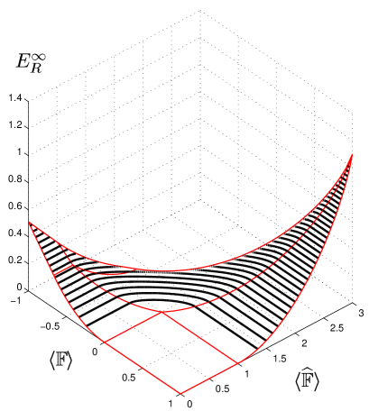
Figure 5: Contour plot of the AREEP $E_{R}^{\infty}$ for the OO-invariant states, parameterized by $f$ and $\hat{f}$ ($d=3$). Superimposed on this plot are the lines separating the different regions defined in the text (regions $A$, $B$ and $C$, the PPT set, the set of additive states and the regions AYCD and CYB).

VII Conclusion

In this paper, we have considered the calculation of the AREEP $E_{R}^{\infty}$ for the class of OO-invariant states, generalizing the results of ka , which dealt only with the class of Werner states. This has been achieved using four basic ingredients: properties of the REEP $E_{R}$, properties of the Rains bound $R$ (1), and a deep connection between these two quantities $E_{R}^{\infty}$ and $R$. The final cornerstone of the calculation is the symmetry inherent in the OO-invariant states vollbrecht1 .

The relevant properties of the REEP are that it is an additive entanglement measure in a large region of state space Rains_Lemma and that the AREEP is convex everywhere rudolph . This convexity allows us to use the “minimal convex extension” construction as a lower bound.

We have shown here that the Rains bound is also convex and continuous, and that the calculation of it can be reformulated as a convex optimization problem, which implies, by the way, that this problem can be solved efficiently and does not suffer from multiple local optima.

We have also made explicit the techniques that were already employed in ka implicitly, resulting in Lemma 4. This Lemma shows that there is a deep connection between the AREEP and the Rains bound and seems to suggest that both regularise to the same quantity rains_private . Unfortunately, in its current form, the Lemma is weakened by the additional requirement on the states $\sigma$, over which the Rains bound is minimized, that the quantity $|\sigma^{T_{2}}|^{T_{2}}$ should be positive. We have coined the term binegative states for those states that violate this requirement and we have made some initial investigations into the question of their existence. Specifically, we showed that for the case of OO-invariant states, $\sigma$ is not binegative, so that the Lemma can be used here at full strength. If it turned out that the extra requirement can always be removed, in one way or another, then the Lemma could directly be used to prove Rains’ suggestion that $E_{R}^{\infty}=R^{\infty}$.

For the time being, we have been able to show that at least for $E_{R}$-additive states $\rho$, the Rains bound and the REEP are equal (and, of course, also equal to their regularised versions).

Using these results, we have calculated the AREEP for OO-invariant states and it followed as a by-product of the calculation that the Rains bound is identical to $E_{R}^{\infty}$ for the OO-invariant states.

This last result could be taken as a hint that the Rains bound might be additive everywhere, in contrast to $E_{R}$. If this were true, then this would imply that the AREEP is precisely equal to the (non-regularised) Rains bound and, furthermore, that it can be calculated efficiently.

This work has been supported by project GOA-Mefisto-666 (Belgium), the EPSRC (UK), the European Union project EQUIP, the Deutsche Forschungsgemeinschaft (Germany) and the European Science Foundation. KA wishes to thank J. Eisert, M. Plenio, F. Verstraete, J. Dehaene and E. Rains for fruitful discussions and remarks.

References

- (1) P. Horodecki and R. Horodecki, Quant. Inf. Comp. 1, 45 (2001); R.F. Werner, Quantum information – an introduction to basic theoretical concepts and experiments, in Springer Tracts in Modern Physics 173 (Springer, Heidelberg, 2001); W.K. Wootters, Quant. Inf. Comp. 1, 27 (2001); M.A. Nielsen and G. Vidal, Quant. Inf. Comp. 1, 76 (2001); M.B. Plenio and V. Vedral, Cont. Phys. 39, 431 (1998).
- (2) R.F. Werner, Phys. Rev. A 40, 4277 (1989).
- (3) V. Vedral, M.B. Plenio, M.A. Rippin, and P.L. Knight, Phys. Rev. Lett. 78, 2275 (1997); V. Vedral and M.B. Plenio, Phys. Rev. A 57, 1619 (1998); V. Vedral, M.B. Plenio, K.A. Jacobs, and P.L. Knight, Phys. Rev. A 56, 4452(1997).
- (4) E. Rains, Phys. Rev. A 60, 179 (1999). Erratum: Phys. Rev. A 63, 019902 (2001).
- (5) E. Rains, IEEE Trans. Inf. Theory 47(7), 2921–2933, 2001.
- (6) K.G. H. Vollbrecht and R.F. Werner, Phys. Rev. A 64, 062307 (2001).
- (7) E. Rains, private communication (2001).
- (8) M. Ohya and D. Petz, Quantrum Entropy and its Use, Springer-Verlag, 1993.
- (9) M. Donald, M. Horodecki and O. Rudolph, Lanl e-print 0105017.
- (10) K. Audenaert, J. Eisert, E. Jané, M.B. Plenio, S. Virmani and B. De Moor, Phys.Rev.Lett. 87, 217902, 2001.
- (11) M. Donald and M. Horodecki, Phys.Lett. A 264, 257–260 (1999).