State permutations from manipulation of near level-crossings.

Abstract

We discuss some systematic methods for implementing state manipulations in systems formally similar to chains of a few spins with nearest-neighbor interactions, arranged such that there are strong and weak scales of coupling links. States are permuted by means of bias potentials applied to a few selected sites. This generic structure is then related to an atoms-in-a-cavity model that has been proposed in the literature as a way of achieving a decoherence free subspace. A new method using adiabatically varying laser detuning to implement a CNOT gate in this model is proposed.

I Introduction

Two central concerns of quantum information theory are representation of data through occupancy of quantum states and the manipulation of these data. Roughly speaking, for these purposes, we desire systems that have the two properties:

1) When the system is left alone it should have some eigenstates that are quite localized, in the sense that the occupancy of such a state identifies a property of a localized physical element (e.g., a particular spin being up or down, or a state of a single atom being in one energy level or the other. )

2) There is a simple mechanics for applying a signal from the outside that will move the system from one of these “localized” states to another.

In this paper we discuss two models that show some interesting potentialities for this program. The first is a novel and rather idealized “spin chain” type of model; the second is an “atoms-in-a cavity” model, still quite idealized, that has been discussed at some length in several previous works by other authors.

All of the models that we shall consider (and some others in the literature) have a unifying feature that can be stated as a nearly-general property of a class of Hamiltonians. We define this class as follows:

a) We picture the states as points distributed in a space, and connect each pair of points that correspond to a non-vanishing matrix element of $H$. We consider only cases in which each point is connected to a few neighbors. A natural extension that will be required for the atoms-in-a-cavity discussion is to include the “environment” as one of the points in the space, with dissipative links to it from some of the other states.

b) Now let there be two scales of strength in these connections, strong (S) and weak (W). If there are small neighborhoods, or blocs, in this space in which all connections, as well as the diagonal elements, are weak, then there will generally be energy eigenfunctions that are nearly confined to these blocs. This can be seen by treating the weak links to the outside perturbatively after diagonalizing the weak bloc in the absence of connections to the outside. Since the denominators in this perturbation are generally of strong order and the numerators of weak order, the perturbation will make little difference to the state. We can characterize the perturbation of the state as being of order ${\rm W/S}$. Likewise, we note that although other weak blocs somewhere else in the space of states will indeed have energies of weak scale, we are in general protected from a small denominator by the fact that we must go through a weak link to get from the first bloc into an intervening strong bloc, and then another weak link to get to the second weak bloc, where we would find energies of the weak order characterizing the first bloc. Thus the largest term with a dangerous denominator would generally be of order ${\rm W^{2}/SW}$. (The dissipative connections to the environment in the atoms-in-a-cavity model to be considered later will come to be classified as, effectively, a set of additional strong links.)

The above statement is, to be sure, neither a theorem nor an unfamiliar kind of conclusion. In much more sophisticated work on infinite systems much is known about the relations between disorder and localization. But we will show that the result above, tempered as it is with “generally” (meaning “most of the time”) is a very useful design criterion for systems that meet the objectives enunciated at the beginning of this paper.

We will begin by considering cases where the strong bloc consists of two states connected by a single strong link, such that the Hamiltonian is of the form

$$\left(\begin{array}[]{cc}0&S\\ S&0\end{array}\right),$$ (1)

and the eigenvalues of the two energy eigensates are $\pm S$. Adding weak scale connections to other states, will make only a small perturbation to these eigenstates. We may generalise this to chains of an arbitrary even number of states connected by strong links of similar size – all the eigenvalues will be of order strong. However, if we have an odd number of states, there will always be a zero eigenvalue, for example, three states connected via a Hamiltonian of the form

$$\left(\begin{array}[]{ccc}0&S_{12}&0\\ S_{12}&0&S_{23}\\ 0&S_{23}&0\end{array}\right),$$ (2)

will have eigenvalues $\{0,\pm\sqrt{S_{12}^{2}+S_{23}^{2}}\}$. Due to the presense of a zero eigenvalue, adding weak scale links to states outside of this bloc will greatly perturb the eigenstates. We regain of a set of eigenvalues, all of strong order, however, if we introduce either a coupling $S_{13}$ between the 1st and the 3rd states, or diagonal elements of strong scale. Dissipative connections, for example, would enter as imaginary diagonal terms.

Once we have reason to take a weak bloc as isolated, we then wish to address the movements of probability through the action of time dependent external interventions. In the first chain-of-spins model that we shall present, with five sites, this will take the form of a bias signal to be applied to the middle site, which is changed slowly enough for adiabaticity of a kind to be realized. The actual state transformations that we discuss can be regarded as fairly elaborate “avoided-crossing” phenomena. In the atoms-in-a-cavity models of Refs. beige1 , beige2 , and pachos that we consider, after noting how the creation therein of a decoherence-free subspace can be qualitatively understood using the strong-weak picture, we demonstrate an adiabatic method of manipulation by tuning and detuning that is different from the pulsed, and exactly-timed, laser techniques that are suggested in these references.

The remainder of this paper is structured thus: The next section analyses spin-chain models with a W and S hierarchy of nearest-neighbor couplings and time-dependent biases on selected sites. Section III then re-examines atoms-in-a-cavity models, while Sec. IV provides further discussion and a conclusion.

II Spin-chain models

Our first example uses a chain of five spins. We take the spins to be numbered consecutively from left to right, with pure exchange interactions built of the operators between adjacent spins $i$ and $j$,

$$h^{(i,j)}=\sigma_{+}^{(i)}\,\sigma_{-}^{(j)}+\sigma_{-}^{(i)}\,\sigma_{+}^{(j)}.$$ (3)

We choose the Hamiltonian

$$H=g_{1}h^{(1,2)}+\lambda h^{(2,3)}+\lambda h^{(3,4)}+g_{2}h^{(4,5)}+f(t)[\sigma_{z}^{(3)}-1],$$ (4)

where we have added a single time-dependent term involving the operator of the middle spin $\vec{\sigma}^{(3)}$. We refer to the function $f(t)$ as the bias on site #3. Since this Hamiltonian commutes with the operator $\sum_{i}\sigma_{z}^{(i)}$, we can operate within the set of five states with four of the spins up and one spin down. The S-W structure comes from taking $\lambda\ll g_{1},g_{2}$, and $g_{1}\neq g_{2}$. When $f(t)=0$, this choice has the effect of creating eigenstates of $H$ that are very nearly the following,

$$\psi_{1} = (\uparrow\downarrow+\downarrow\uparrow)(\uparrow\uparrow\uparrow)/\sqrt{2},$$

$$\psi_{2} = (\uparrow\downarrow-\downarrow\uparrow)(\uparrow\uparrow\uparrow)/\sqrt{2},$$

$$\psi_{3} = (\uparrow\uparrow\downarrow\uparrow\uparrow),$$

$$\psi_{4} = (\uparrow\uparrow\uparrow)(\uparrow\downarrow+\downarrow\uparrow)/\sqrt{2},$$

$$\psi_{5} = (\uparrow\uparrow\uparrow)(\uparrow\downarrow-\downarrow\uparrow)/\sqrt{2}.$$ (5)

We understand these combinations qualitatively by noting that they would be the exact $f=0$ eigenstates if the small coupling $\lambda$ were set to zero, and that, treating $\lambda$ as a perturbation, the link between the pairs of states (#1,#2) and (#4,#5) is of order $\lambda^{2}$.

Now we ask the question: Of the 120 permutations on this set of five states, how many can we implement by applying a small series of simple pulses in $f(t)$? In forming these pulses we shall tailor $f(t)$ to the permutation that is sought, but we shall insist that $f(t)$ begins at and ends at the value zero. By a permutation we mean just the reshuffling of the states, modulo phase. This demand effectively rules out setting relative phases, which would require fine-tuning in any system that is to be considered over a period of time. The answer to the question is “all 120”.

The method uses adiabatic avoided-level-crossing dynamics, with an additional feature that can be embodied in the above Hamiltonian, namely, that the bias on the weakly coupled site can be changed suddenly, without affecting the state of the system appreciably, at all times when the system is far from any (near) level-crossing. As an example, we choose the parameters $g_{1}=30$, $g_{2}=60$, $\lambda=1$, and begin by defining two bias operations $f(t)$,

$$f_{a}(t)=(t-t_{0})\,\,\theta[t-t_{0}]\theta[t_{0}+\tau-t]\rightarrow U_{a}(t_{0}),$$

$$f_{b}(t)=-f_{a}(t)\rightarrow U_{b}(t_{0}).$$ (6)

The signal begins at $t=t_{0}$, grows linearly until $t=t_{0}+\tau$ when it is switched off abruptly. We take $\tau=20$ in the applications that follow. Any bias $f_{\alpha}(t)$ defines a transformation,

$$U_{\alpha}(t_{0})=T[\exp(-i\int_{t_{0}}^{t_{0}+\tau}dt^{\prime}H(t^{\prime}))].$$ (7)

We will show footnote1 that the operation $U_{a}$ effects the permutation $\langle 13\rangle$, while $U_{b}$ effects $\langle 23\rangle$. The turn-off of the bias at $t=t_{0}+\tau$ leaves the state at time $t=t_{0}+\tau$ evolving with the Hamiltonian of Eq. (4) with $f=0$, so that we are prepared to apply another signal to get a compound of the permutations. Thus we can write,

$$U_{1\Leftrightarrow 2}\equiv[U_{a}(2\tau)][U_{b}(\tau)][U_{a}(0)],$$ (8)

where the time arguments emphasize that the transformations are to be executed serially over a total time of $3\tau$. Using the composition property of permutations $\langle 13\rangle\langle 23\rangle\langle 13\rangle=\langle 12\rangle$, we see that $U_{1\Leftrightarrow 2}$ just interchanges states #1 and #2, leaving #3 alone. The basis for anticipating the actions of both the individual and compound transformations can be shown in an averted level-crossing diagram based on Eq. (4) with the bias function given by,

$$f(t)=f_{a}(t)+f_{b}(t-\tau)+f_{a}(t-2\tau).$$ (9)

Figure 1 shows plots of the energy levels for the first three states as they evolve under the above successive changes of the bias.

Figure 1: Level diagrams for the three states that are appreciably affected by the pulse chain of Eq. (9). The numbers on the curves indicate possible initial states, enumerated as in Eq. (5). In the adiabatic limit, the system, beginning in one of these states, follows the continuous path connected thereto. For example, if the system is initially prepared in state #1, then it first adiabatically transforms to state #3, remains there during the sudden bias jump at $t=40$, then adiabatically transforms to state #2. States #4 and #5 remain virtually unmixed and at their original energies. The energy is is units of $\lambda$ and the time in units of $\lambda^{-1}$.

To show that the states really follow these paths, we construct the matrix $U(t)=T[\exp(-i\int_{0}^{t}dt^{\prime}H(t^{\prime}))]$ by directly solving the Schrödinger equation with the time-dependent bias of Eq. (9). In Figs. 2 and 3, we plot $|\langle 1,2,3|U(t)|1\rangle|^{2}$ and $|\langle 1,2,3|U(t)|2\rangle|^{2}$ against time in this solution, giving the expected behavior, $|U(3\tau)|^{2}=|U_{1\Leftrightarrow 2}|^{2}$ with negligible contamination either from non-adiabaticity in the region of small level separation, or from transitions induced in any of the three sudden changes. The plots show clearly the effects of each of the constituent transitions in turn, giving rise to the factorization indicated in Eq. (8).

Figure 2: The evolution of probabilities for the Hamiltonian of Eq. (4) with $f(t)$ from Eq. (9), and the initial state #1. The light solid curve is the probability of the system in state #1 (displaced slightly upward for clarity), the heavy solid curve is for #3, and the dashed curve is for #2 (displaced slightly downward). The time is given in units of $\lambda^{-1}$.

Figure 3: Same as Fig. 2, but with the initial state taken as #2. Together, Figs. 2 and 3 show the interchange operation effected by the particular pulses of (9). The time is given in units of $\lambda^{-1}$.

To implement the transformations involving states #4 and #5, we introduce four more bias functions,

$$f_{c}(t) = 2(\tau-t)\theta(\tau-t)\theta(t)\rightarrow U_{c}\rightarrow\langle 352\rangle,$$

$$f_{d}(t) = -f_{c}(t)\rightarrow U_{d}\rightarrow\langle 341\rangle,$$

$$f_{e}(t) = -2(\tau-t/2)\theta(\tau-t)\theta(t)\rightarrow U_{e}\rightarrow\langle 34\rangle,$$

$$f_{f}(t) = -f_{e}(t)\rightarrow U_{f}\rightarrow\langle 35\rangle,$$ (10)

where, for simplicity, we have chosen $t_{0}=0$. By straightforward multiplication of the operations in Eqs. (6) and (10), we obtain $U_{d}U_{a}\!\!\rightarrow\!\!\langle 14\rangle$, $U_{c}U_{b}\!\!\rightarrow\!\!\langle 25\rangle$, $U_{a}U_{f}U_{a}\!\!\rightarrow\!\!\langle 15\rangle$, $U_{b}U_{e}U_{b}\!\!\rightarrow\!\langle 24\rangle$, $U_{e}U_{f}U_{e}\!\!\rightarrow\!\!\langle 45\rangle$. These five composite operations, together with $U_{a}U_{b}U_{a}\!\!\rightarrow\!\!\langle 12\rangle$ and the four single pulse operations $U_{a},U_{b},U_{e},U_{f}$, give all of the simple interchanges. All permutations can be built from these interchanges, although in most cases it would be more efficient to draw on the cycle-of-three permutation operators $U_{c}$ and $U_{d}$ as well, or on further primary pulse shape variants that directly embody other operators.

Now we consider longer chains with nearest neighbor couplings,

$$H_{0}=\sum_{i=j+1}g_{i,j}h^{(i,j)}-E_{0},$$ (11)

where $g_{i,j}$ are coupling coefficients, and $E_{0}$ is the energy that gives $\langle H_{0}\rangle=0$ for the case of all spins up. We again adopt two scales of coupling strength: S and W. As an example, we consider the pattern of couplings $\{g_{1,2},\,\,g_{2,3},\,\,g_{3,4},\ldots\}$ to be {S, W, W, S, W, W, S, W, W, …}. Under this scheme, the states #3,#6,#9… are only weakly coupled to their neighbors.

As before, we take only states with one spin down and the remainder up. With the W coupling constants turned off, the eigenvalues of the states in which the down spin occupies one of the large blocs, i.e., {(#1,#2), (#4,#5), (#7,#8) …}, come in pairs of $\pm g_{i,i+1}$. We assume that the S couplings are sufficiently irregular so that the differences in energies between nearest strong blocs, e.g., $g_{1,2}\!-\!g_{4,5}$, are still of the strong (S) scale. When we add the W couplings, the eigenvectors will remain almost localized, as can be seen from a perturbation expansion. In general, as argued previously, small energy differences between two non-adjacent blocs are not a concern, since as we move across $n$ additional weak links we can tolerate energy denominators that are smaller by a factor of $(g_{W}/g_{S})^{2n}\ll 1$.

Thus for most cases the eigenvectors can be arranged in a list $\{(\xi_{1},\uparrow,\uparrow,\uparrow,...),\,\ (\eta_{1},\uparrow,\uparrow,\uparrow,...),\,\ (\uparrow,\uparrow,\downarrow,\uparrow,\uparrow,...),\,\ (\uparrow,\uparrow,\uparrow,\xi_{2},\uparrow,...),\,\ (\uparrow,\uparrow,\uparrow,\eta_{2},\uparrow,...),\,\ (\uparrow,\uparrow,\uparrow,\uparrow,\uparrow,\downarrow,\uparrow,...),\,\ ...\}$. Here, the $\xi$’s and $\eta$’s stand for the symmetric and anti-symmetric two-component eigenstates of the strong blocs with one spin up and the other down. If the system begins with all of its amplitude in one bloc, the amplitude will stay almost within that bloc under the evolution governed by $H_{0}$.

Now, generalizing the earlier five-site example, we can ask whether biases placed at every third site, #3, #6, #9, …, which are weakly coupled both to the right and to the left, have the capability of moving information around the whole system. We have looked at an eight-site example, with independently manipulable biases at sites #3 and #6. In complete analogy with the five-site case, we find it is easy, for example, to move one of the (#1,#2) eigenstates successively to the blocs (#3), (#4,#5), (#6), (#7,#8), again by numerically solving the Schrödinger equation for the system.

As a qualitative summary of these outcomes, we restate and sharpen some of the remarks in the introduction:

(1) If we have a chain of blocs of states connected, one to another, through an intermediary state that is weakly coupled to both blocs, the dynamics within the blocs will be nearly self-contained. That is, if the probability is localized within a particular bloc at a particular time, in the form of any superposition of the eigenstates belonging to that bloc, then the probability will remain in that bloc. Likewise, a bloc of several states in which the mutual couplings and the diagonal elements are weak will, in general, not admix appreciably with strongly coupled states to its left or right.

(2) By putting controllable biases on a weak connection site to bring the energy of an associated level to (nearly) coincide with a level in an adjacent strong bloc, shifts of probability from bloc to bloc can be implemented in an orderly and complete fashion.

III Atoms-in-a-cavity models

An exact analogue to the above mechanics for moving a system from one state to another can be applied to some models of atoms-in-a-cavity type that have been the subject of a series of recent papers. As an example, we consider the model of Ref.beige1 , with two identical atoms in a cavity, and a dynamics that is effectively confined to three states, which form a decoherence free subspace (DFS).

In this model, the two atoms have three levels, $\{0,1,2\}$, and are placed in a cavity tuned exactly to the $1\!-\!2$ level spacing, with the atoms separately addressable by weak laser fields that drive Rabi oscillations. The cavity mode, if excited, is also allowed to escape through conversion to photons at a partially transmitting wall. This is the only decohering process. The connection scheme for the relevant states is depicted in Fig.4.

Figure 4: In a notation close to that of Ref. beige1 , the states are labeled as $|{\rm atom}\,\#1,{\rm atom}\,\#2\rangle_{\rm cav}$ where “cav” is the excitation of the cavity mode. The states denoted “s” and “a” (for the atomic part) are $|{\rm s,a}\rangle=(|1,2\rangle\pm|2,1\rangle)/\sqrt{2}$. The connections are those variously induced by the three laser couplings and the cavity mode, as explained in the text.

The excitation of the cavity mode from the states in the chain that are coupled thereto are the S links, denoted by fat double arrows. The thin double arrows are W links, and the double arrows leading to D represent the cavity mode leakage to the outside. All W links come from the laser interactions, which are three-fold: on atom #2, an exactly tuned $0\!\leftrightarrow\!2$ signal and an exactly tuned $1\!\leftrightarrow\!2$ signal; on atom #1, just an exactly tuned $1\!\leftrightarrow\!2$ signal, $180^{\circ}$ out of phase with the corresponding signal on the other atom.

The structure shown in Fig. 4 has a general property in common with the models discussed above; there is a bloc within which all connections are weak,

$$|1,1\rangle_{0}\leftrightarrow|a\rangle_{0}\leftrightarrow|1,0\rangle_{0},$$ (12)

characterized in Ref.beige1 as a DFS. The existence of this DFS is explained qualitively in the diagram of Fig.4. In this model both the cavity mode coupling (thick arrows connecting states) and the cavity mode decay (labelled $D$) are of order “strong”. The cavity mode decay is necessary for obtaining the DFS, since in its absence the strongly coupled block by itself

$$|1,1\rangle_{2}\Leftrightarrow|s\rangle_{1}\Leftrightarrow|2,2\rangle_{0}$$ (13)

has a zero eigenvalue. With the dissipative links, $D$, included through imaginary diagonal terms in the Hamiltonian matrix, all three eigenvalues are of “strong” level, and are thus approximately decoupled from the three states $\{|1,1\rangle_{0},|a\rangle_{0},|1,0\rangle_{0}\}$ which form a DFS, as emphasized in Ref.beige1 .

Ref.beige1 proceeds from this observation to the construction of a CNOT gate in which the transformation of states is effected by means of accurately timed laser pulses. We now demonstrate the action of an alternative mechanism for the controlled transformation of the states, following an exact analogue of the protocol used in the first example in this paper. In this mechanism the applied laser fields are slowly changed in frequency, rather than turned on and off.

To show this, we first write an effective Hamiltonian operating within the bloc of Eq. (12), as given in Ref.beige1 , but allowing the laser frequencies to be detuned by a small amount,

$$H_{\rm eff}\!=\!\frac{\Omega}{2}\left[e^{i\Delta_{A}t}|1,0\rangle_{0}\langle a|_{0}-e^{i\Delta_{B}t}|a\rangle_{0}\langle 1,1|_{0}\right]+{\rm h.c.}.$$ (14)

Here $\Omega$ is a Rabi frequency, and the detunings of the $0\!\leftrightarrow\!2$ and $1\!\leftrightarrow\!2$ lasers are given by $\Delta_{A}$ and $\Delta_{B}$ respectively. Transition probabilities in the indicated basis will be unaffected by the transformation (acting in the atomic space only), $\Psi^{\prime}(t)=\exp(-i\Lambda t)\Psi(t)$, where

$$2\Lambda\! = \!({\Delta_{A}\!+\!\Delta_{B}})|1,0\rangle\langle 1,0|\ +\ ({\Delta_{B}\!-\!\Delta_{A}})|a\rangle\langle a|$$ (15)

$$-\ ({\Delta_{A}\!+\!\Delta_{B}})|1,1\rangle\langle 1,1|,$$

giving the new effective Hamiltonian,

$$H^{\prime}_{\rm eff}=\Lambda+\frac{\Omega}{2}[|1,0\rangle_{0}\langle a|_{0}-|a\rangle_{0}\langle 1,1|_{0}]+{\rm h.c.}$$ (16)

This is exactly the first example of the present paper, with the five states reduced to three by taking only the symmetric states in place of the (#1,#2) and (#4,#5) complexes. We may thus interchange the states, exactly as before, by adiabatically varying the detunings. For example, by adiabatically changing the combination ${\Delta_{A}\!+\!\Delta_{B}}$, while keeping ${\Delta_{A}\!-\!\Delta_{B}}$ constant, we can effect the interchange of the states $|1,1\rangle_{0}$ and $|1,0\rangle_{0}$, thus performing a CNOT operation.

The full set of equations describing the evolution of all the states depicted in Fig.4 is given below, where we have used the Hamiltonian from Ref.beige1 and added detuning as in Eq.16:

$$\dot{c}_{|a\rangle_{0}} = -\frac{i\Omega}{2}\left(c_{|10\rangle_{0}}-c_{|11\rangle_{0}}+c_{|22\rangle_{0}}\right)$$

$$\quad\quad-\frac{i}{2}\left(\Delta_{A}-\Delta_{B}\right)c_{|a\rangle_{0}},$$

$$\dot{c}_{|10\rangle_{0}} = -\frac{i\Omega}{2}\left(c_{|a\rangle_{0}}+\frac{1}{\sqrt{2}}c_{|2,0\rangle_{0}}+c_{|s\rangle_{0}}\right)$$

$$\quad\quad-\frac{i}{2}\left(\Delta_{A}+\Delta_{B}\right)c_{|10\rangle_{0}},$$

$$\dot{c}_{|11\rangle_{0}} = -\frac{i\Omega}{2}c_{|a\rangle_{0}}+\frac{i}{2}\left(\Delta_{A}+\Delta_{B}\right)c_{|11\rangle_{0}},$$

$$\dot{c}_{|s\rangle_{0}} = -\frac{i\Omega}{2}c_{|10\rangle_{0}}+\sqrt{2}gc_{|11\rangle_{1}},$$

$$\dot{c}_{|11\rangle_{1}} = \sqrt{2}gc_{|s\rangle_{0}}-\kappa c_{|11\rangle_{1}},$$

$$\dot{c}_{|s\rangle_{1}} = g\left(c_{|22\rangle_{0}}-\sqrt{2}c_{|11\rangle_{2}}\right)-\kappa c_{|s\rangle_{1}},$$

$$\dot{c}_{|22\rangle_{0}} = \frac{i\Omega}{2}\left(c_{|a\rangle_{0}}-\sqrt{2}c_{|20\rangle_{0}}\right)-gc_{|s\rangle_{1}},$$

$$\dot{c}_{|20\rangle_{0}} = -\frac{i\Omega}{2}\left(\frac{1}{\sqrt{2}}c_{|10\rangle_{0}}-\sqrt{2}c_{|22\rangle_{0}}\right)-gc_{|10\rangle_{1}}$$

$$\dot{c}_{|10\rangle_{1}} = gc_{|20\rangle_{0}}-\kappa c_{|10\rangle_{1}},$$

$$\dot{c}_{|11\rangle_{2}} = \sqrt{2}gc_{|s\rangle_{1}}-2\kappa c_{|11\rangle_{2}}.$$ (17)

In these equations, $g$ is the parameter setting the strong scale depicted by the fat double-arrows in Fig. 4, while $\kappa$ sets the (strong) scale of the dissipative links $D$ to the environment (decay of cavity modes).

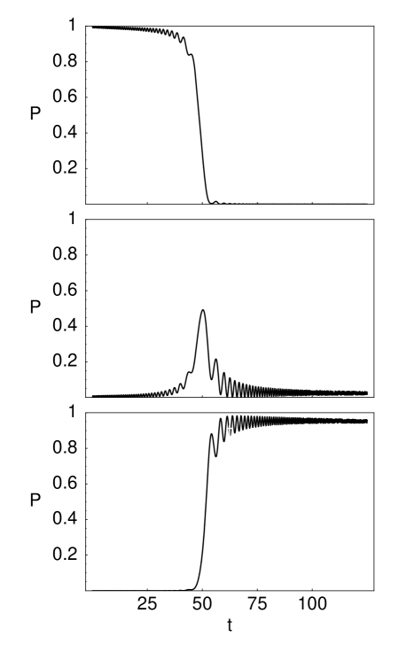
Figure 5: The top panel shows the survival probability of the initial state $|10\rangle_{0}$, the center panel $|a\rangle_{0}$, and the lower panel $|11\rangle_{0}$. The horizontal axis displays time in units of $\Omega^{-1}$. We have taken the parameters $\kappa=g=2000\Omega$, $\Delta_{A}=(10-0.2t)\Omega$ and $\Delta_{A}=(10-0.2t)\Omega$. The CNOT opertation is implemented by adiabatically changing the detunings $\Delta_{A}+\Delta_{B}$ while keeping $\Delta_{A}-\Delta_{B}$ constant.

We have solved this set of equation numerically, to demonstrate the interchange of states $|10\rangle_{0}\leftrightarrow|11\rangle_{0}$. We begin with a steady situation in which detuning parameters $\Delta_{A}$ and $\Delta_{B}$ are substantially greater than $\Omega$, and the initial state is (very stably) either $|1,1\rangle_{0}$ or $|1,0\rangle_{0}$. Then the detuning is manipulated, using simultaneous slow changes of both laser frequencies in order to interchange these two states, in a process similar to those described in section II. The evolution is shown graphically in Fig.5. By contrast, Ref.beige1 uses the perfectly tuned case $\Delta_{A,B}=0$, and takes $\Omega=0$ until a pulse turn-on time. The pulse is then turned off at exactly the time for the interchange $|1,0\rangle_{0}\!\leftrightarrow\!|1,1\rangle_{0}$ to have occurred under the influence of precession alone. In either method, the transformation represents a CNOT gate, the states $|0,1\rangle_{0}$ and $|0,0\rangle_{0}$ being frozen due to the S-W effect. Note that our implementation does not require accurate timing of applied fields.

IV Discussion and conclusion

We have shown that in systems with appropriate arrangements of strong (S) and weak (W) couplings, variable potentials applied to a relatively small number of sites can efficiently effect state permutations for spin chains with pure-exchange coupling. Using the same approach, we found a new way to implement a CNOT gate in an atoms-in-a-cavity model discussed by previous authors beige1 .

A number of models similar to that of Ref. beige1 can be found in the recent literature itano ; block ; beige2 ; facchi ; pachos ; jane . For many of these cases, the generic S-W paradigm developed in the present paper provides a unified basis for understanding how isolated subspaces are generated.

As our final comment we note that the S-W non-dissipative links, and decay-induced dissipation – the two cases specifically studied here – are not the only means by which subspaces can become mutually isolated. For instance, Ref. stodolsky and many subsequent works have discussed cases in which rapid incoherent scattering can freeze a system in a single state or subspace of states.

References

- (1) Permutations are denoted by , where, e.g., implies , , .
- (2) A. Beige, D. Braun, B. Tregenna, and P. L. Knight, Phys. Rev. Lett. 85, 1762 (2000).
- (3) B. Tregenna, A. Beige, P. L. Knight, Phys. Rev. A 65, 032305 (2002).
- (4) J. Pachos and H. Walther, Phys. Rev. Lett. 89, 187903 (2002).
- (5) If the laser-induced couplings and the cavity mode coupling were all of the same order of magnitude as the dissipation through leakage D, then a system initially within the subspace of Eq. (12) would flow rapidly to the modes at the edges of Fig. 4, and out the door D.
- (6) P. Facchi and S. Pascazio, Phys. Rev. Lett. 89, 080401 (2002)
- (7) E. Jané, M. B. Plenio, and D. Jonathan, Phys. Rev. A 65, 050302 (2002).
- (8) R. A. Harris and L. Stodolsky, Phys. Lett. 116B, 464 (1982).
- (9) W. M. Itano, D. J. Heinzen, J. J. Bollinger, and D. J. Wineland, Phys. Rev. A 41, 2295 (1990).
- (10) E. Block and P. R. Berman, Phys. Rev. A 44, 1466 (1991).