Mode structure and photon number correlations in squeezed quantum pulses

Abstract

The question of efficient multimode description of optical pulses is studied. We show that a relatively very small number of nonmonochromatic modes can be sufficient for a complete quantum description of pulses with Gaussian quadrature statistics. For example, a three-mode description was enough to reproduce the experimental data of photon number correlations in optical solitons [S. Spälter et al., Phys. Rev. Lett. 81, 786 (1998)]. This approach is very useful for a detailed understanding of squeezing properties of soliton pulses with the main potential for quantum communication with continuous variables. We show how homodyne detection and/or measurements of photon number correlations can be used to determine the quantum state of the multi-mode field. We also discuss a possible way of physical separation of the nonmonochromatic modes.

I Introduction

For a complete quantum description of an optical pulse, one has to use a multimode density matrix. The question is, how many modes are necessary for such a description. If one works with monochromatic modes, then an infinite number of modes would be needed, which is impractical. On the other hand, one can construct different sets of modes as linear combinations of the monochromatic modes TG66 . These modes (which are however nonmonochromatic) may be more suitable for the quantum description of pulses. In particular, it would be useful to find such a modal structure so that the quantum state of the pulse can be described by the density operator $\hat{\varrho}$ $=$ $\hat{\varrho}_{\rm exc}\otimes\hat{\varrho}_{\rm vac}$, where $\hat{\varrho}_{\rm exc}$ is some nontrivial density operator of a few modes and $\hat{\varrho}_{\rm vac}$ is the vacuum state density operator of all the remaining modes. Thus, we could work with a concise description of the pulse by means of $\hat{\varrho}_{\rm exc}$.

Our work is motivated by the question how to completely describe the quantum state of solitons in optical fibers. Such soliton pulses are used in various schemes of quantum information processing (for a review see, e.g., Natasa ). Can a single-mode description of a soliton pulse be sufficient? When explaining squeezing in the Kerr medium, one sometimes plots a picture of phase space where a quantum uncertainty circle is deformed into an ellipse—a description which clearly corresponds to a single mode situation. This approach is useful to qualitatively understand the generation of continuous variables entanglement as in Silberhorn , but do we use all the quantum features of a given pulse if we treat it as a single mode object? Should one, instead, work with many more modes of a pulse in the hope that each of them can become a useful resource for quantum communication? Multi-mode correlations of photon numbers in a soliton were observed SKKSL98 . To numerically calculate such correlations, quantum variables of a soliton were treated on a position grid of typically $\sim 10^{2}-10^{3}$ points Spaelter-dis ; SKW99 . Are there hundreds of useful modes available in a pulse, or would a better choice of the mode functions show that only a few modes (perhaps just one?) are in some nontrivial quantum state? Or are just four quantum operators introduced by Haus and Lai HausLai sufficient to describe all the relevant phenomena?

Knowing the answer to the question of what is the complete quantum description of a pulse would be very helpful in quantum information processing: one could fully utilize the squeezing and entanglement properties of our sources. After forming a soliton pulse in a fiber, one can determine its multimode quantum state in the most comprehensive way. One can then optimize the medium properties to achieve maximum squeezing, or maximum purity of an entangled state. Working with pairs of correlated pulses, one could apply a proper measurement scheme and use entanglement criteria for multimode bipartite Gaussian states EntCrit to check wheteher the pulse pair is entangled or separable. One can also better understand the influence of the medium on the propagating pulse: provided that the output pulse is deformed, what happens with the quantum information carried by the pulse? Is it washed out by decoherence processes (or perhaps by an eavesdropper), or is it just unitarily transformed into other modes of the same pulse? A simple and correct measurement and description of the multimode state is highly desirable.

This work is organized as follows. In Sec. II we introduce nonmonochromatic modes and deal with the transformations between different sets of quadrature operators. Sec. III studies basic properties of the photon statistics of multimode fields: mean photon numbers and covariances between different modes. In Sec. IV we discuss a homodyne scheme for a complete determination of Gaussian states of nonmonochromatic multi-mode fields. In Sec. V we compare the photon number squeezing available via applying a proper local oscillator modulation and via using spectral filtering. Sec. VI suggests a way for an optimal selection of the nonmonochromatic mode functions. In Sec. VII we discuss a possible way how to physically separate individual nonmonochromatic modes of the pulse. Discussion and conclusion are presented in Sec. VIII. Most of the mathematical details are discussed in Appendixes A–E, and in App. F we compare our approach to that of Haus and Lai HausLai .

II Nonmonochromatic modes

Under the term “mode” we understand a single degree of freedom of the electromagnetic field; a mode can be described by a pair of bosonic operators. It can be monochromatic (evolution described by a single frequency) or nonmonochromatic. Any state of the field can be treated in different mode decompositions. In a given decomposition the state is called single mode if all modes except of one have vacuum statistics of their operators, in the opposite case the state is multimode. In this section we deal with the transition between different mode decompositions.

II.1 Bosonic operators

Let us assume polarized optical field propagating in a given direction. The monochromatic modes of the field are denoted by the corresponding frequency $\omega$, and the bosonic operators of these modes satisfy the commutation relations

$$[\hat{a}(\omega),\hat{a}^{{\dagger}}(\omega^{\prime})]=\delta(\omega-\omega^{\prime}),\qquad[\hat{a}(\omega),\hat{a}(\omega^{\prime})]=0.$$ (1)

Let us assume a complete orthonormal set of functions $f_{k}(\omega)$,

$$\int f_{m}^{*}(\omega)f_{k}(\omega)d\omega=\delta_{mk},$$ (2)

$$\sum_{k}f_{k}^{*}(\omega)f_{k}(\omega)=\delta(\omega-\omega^{\prime}).$$ (3)

We define a new set of operators $\hat{b}_{k}$ as

$$\hat{b}_{k}=\int f_{k}(\omega)\hat{a}(\omega)d\omega$$ (4)

which satisfy the commutation relations

$$[\hat{b}_{k},\hat{b}_{k^{\prime}}^{{\dagger}}]=\delta_{kk^{\prime}},\qquad[\hat{b}_{k},\hat{b}_{k^{\prime}}]=0.$$ (5)

Thus, the functions $f_{k}(\omega)$ can be used to define a new set of nonmonochromatic modes. The inverse transformation of the nonmonochromatic modes to the monochromatic ones reads

$$\hat{a}(\omega)=\sum_{k}f^{*}_{k}(\omega)\hat{b}_{k}.$$ (6)

II.2 Example

Let us consider a pulse with a normalized frequency envelope $f(\omega)$; $\int|f(\omega)|^{2}d\omega$ $=$ 1. Let us define an orthonormal system of mode functions as in Eqs. (2) and (3) with $f_{1}(\omega)\equiv f(\omega)$. Let the quantum state of the first mode $\hat{b}_{1}$ be a coherent state $|\beta\rangle_{1}$, $\hat{b}_{1}|\beta\rangle_{1}$ $=$ $\beta|\beta\rangle_{1}$, and let all the other $b$-modes be in vacuum $|0\rangle_{k}$, $\hat{b}_{k}|0\rangle_{k}$ $=$ 0, $k>1$. By means of the transformation (6) we find that using the monochromatic modes, the quantum state is a multi-mode coherent state $\prod_{\omega}|f(\omega)\beta\rangle_{\omega}$. Even though the single-mode and multimode coherent states are related to the same object, i.e., a pulse in a coherent state, the single-mode description is clearly more convenient for handling and for understanding the field structure. Of course, for other than coherent states the transformations of the state in different mode-systems are not so straightforward, but still can provide us with a very convenient way of the quantum state description.

II.3 Quadrature operators

We define the hermitian quadrature operators $\hat{x}(\omega)$, $\hat{p}(\omega)$ as

$$\hat{x}(\omega) = \frac{1}{\sqrt{2}}\left(\hat{a}(\omega)+\hat{a}^{{\dagger}}(\omega)\right),$$ (7)

$$\hat{p}(\omega) = \frac{1}{i\sqrt{2}}\left(\hat{a}(\omega)-\hat{a}^{{\dagger}}(\omega)\right),$$ (8)

and similarly the $b$-mode quadrature operators $\hat{X}_{k}$, $\hat{P}_{k}$ as

$$\hat{X}_{k} = \frac{1}{\sqrt{2}}\left(\hat{b}_{k}+\hat{b}_{k}^{{\dagger}}\right),$$ (9)

$$\hat{P}_{k} = \frac{1}{i\sqrt{2}}\left(\hat{b}_{k}-\hat{b}^{{\dagger}}_{k}\right).$$ (10)

These operators obey the same commutation relations as the quantum mechanical position and momentum operators with $\hbar$ $=$ 1, i.e.,

$$\left[\hat{x}(\omega),\hat{p}(\omega^{\prime})\right]=i\delta(\omega-\omega^{\prime}),$$ (11)

$$\left[\hat{x}(\omega),\hat{x}(\omega^{\prime})\right]=\left[\hat{p}(\omega),\hat{p}(\omega^{\prime})\right]=0,$$ (12)

and

$$\left[\hat{X}_{k},\hat{P}_{k^{\prime}}\right]=i\delta_{kk^{\prime}},$$ (13)

$$\left[\hat{X}_{k},\hat{X}_{k^{\prime}}\right]=\left[\hat{P}_{k},\hat{P}_{k^{\prime}}\right]=0.$$ (14)

The transformation between the two sets of quadrature operators can be written in the form

$$\hat{\mu}_{k} = \sum_{\xi=x,p}\int Z^{\mu\xi}_{k}(\omega)\hat{\xi}(\omega)d\omega,$$ (15)

$$\hat{\xi}(\omega) = \sum_{\mu=X,P}\sum_{k}Z^{\mu\xi}_{k}(\omega)\hat{\mu}_{k}$$ (16)

with $\xi=x,p$, and $\mu=X,P$, and the transformation matrix $Z$ is

$$Z^{Xx}_{k}(\omega)=Z^{Pp}_{k}(\omega)=\text{Re}\ f_{k}(\omega)$$ (17)

$$Z^{Xp}_{k}(\omega)=-Z^{Px}_{k}(\omega)=\text{Im}\ f_{k}(\omega).$$ (18)

As can be checked, matrix $Z$ satisfies the orthogonality relations

$$\sum_{\xi}\int Z^{\mu\xi}_{k}(\omega)Z^{\mu^{\prime}\xi}_{k^{\prime}}(\omega)d\omega=\delta_{\mu\mu^{\prime}}\delta_{kk^{\prime}},$$ (19)

$$\sum_{\mu}\sum_{k}Z^{\mu\xi}_{k}(\omega)Z^{\mu\xi^{\prime}}_{k}(\omega^{\prime})=\delta(\omega-\omega^{\prime})\delta_{\xi\xi^{\prime}}.$$ (20)

Sometimes it is useful to work with a discrete set of frequencies $\omega_{j}$ corresponding to frequency bins of width $\Delta\omega$. Quadrature $\hat{\xi}_{j}$ of the $j$th bin is obtained as

$$\hat{\xi}_{j}=\sum_{\mu=X,P}\sum_{k}Z^{\mu\xi}_{kj}\hat{\mu}_{k},$$ (21)

where the transformation matrix elements $Z^{\mu\xi}_{kj}$ are

$$Z^{\mu\xi}_{kj}\equiv Z^{\mu\xi}_{k}(\omega_{j})\sqrt{\Delta\omega}.$$ (22)

For brevity, we can join the quadratures $\hat{x}(\omega)$ and $\hat{p}(\omega)$ into a single vector $\hat{\xi}$, and similarly the quadratures $\hat{X}_{k}$ and $\hat{P}_{k}$ into a single vector $\hat{\mu}$, so that the transformations (15) and (16) [or (21)] are written in the matrix multiplication form

$$\hat{\mu}=Z\hat{\xi},\qquad\hat{\xi}=Z^{T}\hat{\mu}.$$ (23)

Here the superscript $T$ means matrix transposition, and the rows of the matrix $Z$ are represented by indices $\mu$ and $k$, and the columns by the indices $\xi$ and $\omega$ (or $j$).

II.4 Mean quadratures and variances

Important properties of multimode quantum states are given by the vectors of the quadrature mean values, $\overline{\xi}_{j}$ $\equiv$ Tr$[\hat{\varrho}\hat{\xi}_{j}]$ and $\overline{\mu}_{k}$ $\equiv$ Tr$[\hat{\varrho}\hat{\mu}_{k}]$, and by the variance matrices $V$ and $V^{\prime}$, given as

$$V_{\mu k,\mu^{\prime}k^{\prime}} = \frac{1}{2}\left\langle\left\{\left(\mu_{k}-\overline{\mu}_{k}\right),\left(\mu^{\prime}_{k^{\prime}}-\overline{\mu^{\prime}}_{k^{\prime}}\right)\right\}\right\rangle,$$ (24)

$$V^{\prime}_{\xi j,\xi^{\prime}j^{\prime}} = \frac{1}{2}\left\langle\left\{\left(\xi_{j}-\overline{\xi}_{j}\right),\left(\xi^{\prime}_{j^{\prime}}-\overline{\xi^{\prime}}_{j^{\prime}}\right)\right\}\right\rangle$$ (25)

where $\{\dots\}$ stands for the anticommutator, $\{\hat{A},\hat{B}\}$ $\equiv$ $\hat{A}\hat{B}$ $+$ $\hat{B}\hat{A}$, and $\langle\dots\rangle$ represents averaging $\langle\hat{A}\rangle$ $\equiv$ Tr$(\hat{\varrho}\hat{A})$. The relationship between these quantities can be written in the matrix multiplication form as

$$\overline{\mu} = Z\overline{\xi},$$ (26)

$$\overline{\xi} = Z^{T}\overline{\bf\mu},$$ (27)

$$V = ZV^{\prime}Z^{T},$$ (28)

$$V^{\prime} = Z^{T}VZ.$$ (29)

In general, to transform between $\overline{\mu}$, $V$, and $\overline{\xi}$, $V^{\prime}$, one has to know the complete transformation matrix $Z$, i.e., the whole set of mode functions $f_{k}(\omega)$. However, if we assume that only a few nonmonochromatic modes are excited while the rest is in vacuum state, then the explicit form of the empty mode functions does not play any role. (It was also illustrated in the Example II.2 where only one mode function $f(\omega)$ was enough to transform the state into the multi-mode case.) This can be used for a simplified calculation of the transformed quantities, as discussed in App. A.

III Photon statistics of multimode Gaussian states

Among all possible states, the class of Gaussian states is one of the most important—both from the theoretical and experimental point of view. The basic property of these states is that their Wigner function (as well as the $Q$-function or the characteristic function) have Gaussian form (see, e.g., SMD94 ; EntCrit ; Reconstr ). Examples of Gaussian states are coherent states, squeezed coherent states, thermal states, and squeezed thermal states. Gaussian states are typically observed in most experiments with optical pulses. In this paper we confine ourselves to Gaussian states; the main advantage used here is that a Gaussian state remains Gaussian in any mode decomposition and a relatively small number of parameters is necessary for its description.

III.1 Mean photon numbers and variances

Let us first study the relation between quadrature moments and photon number moments in discrete modes. The photon number operator in $k$th mode $\hat{n}_{k}$ can be expressed by means of the quadrature operators as

$$\hat{n}_{k}=\frac{1}{2}\left(\hat{x}_{k}^{2}+\hat{p}_{k}^{2}-1\right).$$ (30)

The mean photon number in $k$th mode is thus

$$\langle n_{k}\rangle=\frac{1}{2}\left(\langle\hat{x}_{k}^{2}\rangle+\langle\hat{p}_{k}^{2}\rangle-1\right),$$ (31)

and the mean product of photon numbers is

$$\langle n_{k}n_{l}\rangle=\frac{1}{4}\left(\left\langle\hat{x}_{k}^{2}\hat{x}_{l}^{2}\right\rangle+\left\langle\hat{x}_{k}^{2}\hat{p}_{l}^{2}\right\rangle+\left\langle\hat{p}_{k}^{2}\hat{p}_{l}^{2}\right\rangle+\left\langle\hat{p}_{k}^{2}\hat{x}_{l}^{2}\right\rangle\right.$$

$$\left.-\left\langle\hat{x}_{k}^{2}\right\rangle-\left\langle\hat{p}_{k}^{2}\right\rangle-\left\langle\hat{x}_{l}^{2}\right\rangle-\left\langle\hat{p}_{l}^{2}\right\rangle+1\right).$$ (32)

As discussed in App. B, for Gaussian states all the quadrature moments on right hand sides of Eqs. (31) – (32) can be expressed using the quadrature means and variances as in Eqs. (82) – (86). The resulting photon number moments can be used to calculate the photon number covariances

$${\rm cov}\ (n_{k},n_{l})\equiv\langle n_{k}n_{l}\rangle-\langle n_{k}\rangle\langle n_{l}\rangle,$$ (33)

which can be written in terms of the quadrature means and variances as

$${\rm cov}\ (n_{k},n_{l})=\bar{x}_{k}\bar{x}_{l}V^{\prime}_{xk,xl}+\bar{x}_{k}\bar{p}_{l}V^{\prime}_{xk,pl}$$

$$+\bar{p}_{k}\bar{x}_{l}V^{\prime}_{pk,xl}+\bar{p}_{k}\bar{p}_{l}V^{\prime}_{pk,pl}$$

$$+\frac{1}{2}\left(V^{\prime 2}_{xk,xl}+V^{\prime 2}_{pk,xl}+V^{\prime 2}_{xk,pl}+V^{\prime 2}_{pk,pl}\right)-\frac{\delta_{kl}}{4},$$ (34)

with the special case $\Delta n_{k}^{2}$ $\equiv$ cov$(n_{k},n_{k})$. A very important role is played by the so called normally ordered covariance

$$C_{kl}\equiv\langle:\Delta\hat{n}_{k}\Delta\hat{n}_{l}:\rangle=\text{cov}(n_{k},n_{l})-\delta_{kl}\langle n_{k}\rangle.$$ (35)

The normally ordered covariance is used to define the normalized correlation matrix as in SKKSL98 ,

$$C^{\text{(n)}}_{kl} \equiv \frac{\langle:\Delta\hat{n}_{k}\Delta\hat{n}_{l}:\rangle}{\sqrt{\Delta n_{k}^{2}\Delta n_{l}^{2}}}=\frac{C_{kl}}{\sqrt{\Delta n_{k}^{2}\Delta n_{l}^{2}}}.$$ (36)

Values of the correlation matrix measured in SKKSL98 are shown in Fig. 1a. In the limit of continuous frequency modes, one can define photon number density $\langle n(\omega)\rangle$, variance density $\langle\Delta n^{2}(\omega)\rangle$ $=\langle n(\omega)\rangle$, and the normally ordered covariance $C(\omega,\omega^{\prime})$ with its normalized version $C^{\text{(n)}}(\omega,\omega^{\prime})$. Since a Gaussian state remains Gaussian in any mode decomposition, and since the parameters of a Gaussian state $\bar{\xi}$ and $V$ can easily be transformed from one mode decomposition into another, one can also calculate the photon number mean values and correlations in arbitrary mode decomposition.

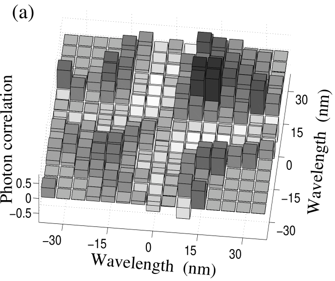
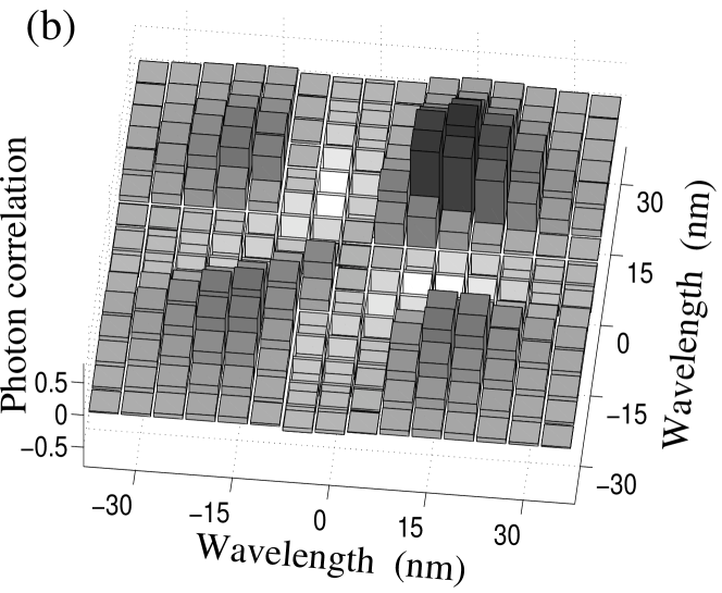
Figure 1: Photon correlation matrix $C^{\text{(n)}}_{kl}$ as a function of the wavelengths of the pulse spectrum. Results measured in SKKSL98 with omitted elements with very large fluctuations ($>0.8$) $(a)$, and the best fit using a reconstructed three-mode variance matrix $V_{Xk,Xk^{\prime}}$ (see Sec. III.4) $(b)$.

III.2 Photon correlations in multimode pulses

If we try to reproduce the experimental results of SKKSL98 as truly as possible with as few modes as possible, the first attempt would be to start with just a single nonmonochromatic mode. However, as shown in Appendix C, the covariance matrix cov$(n_{k},n_{l})$ of such a field would have the same sign for all values $k$ and $l$. The sign would be positive if the single-mode state is super-Poissonian, or negative if the single-mode state is sub-Poissonian. On the other hand, the covariance matrix measured in SKKSL98 contains both positive and negative elements. Therefore, the quantum state of the soliton pulses measured in SKKSL98 cannot be described as a single nonmonochromatic mode.

Exact analytical expressions are rather lengthy if more than one mode are excited. However, relatively simple relations can be obtained if the following requirements are met: $(i)$ The coherent amplitude of at least one of the modes is much greater than any of the variance matrix elements, $(ii)$ only the $X$-quadratures have non-zero mean values, i.e., $\bar{P}_{k}=0$ for all $k$, and $(iii)$ the mode functions are real. While the condition $(i)$ is generally valid for all strong pulses, the conditions $(ii)$ and $(iii)$ are related to our choice of mode functions and their generalization is straightforward. In Eq. (34) the terms containing $\bar{p}_{k,l}$ vanish and the first term on the right is dominant; thus Eq. (34) becomes

$$\text{cov}\ (n_{k},n_{l})\approx\bar{x}_{k}\bar{x}_{l}V^{\prime}_{xk,xl}.$$ (37)

To calculate this quantity using the nonmonochromatic modes, we write

$$\bar{x}_{k}=\sum_{n\leq N}f_{n}(\omega_{k})\bar{X}_{n}\sqrt{\Delta\omega}$$ (38)

(see Eqs. (27), (17), and (22)), and for $V^{\prime}_{xk,xl}$ we use Eq. (76) from Appendix A. The mean photon number is

$$\langle n_{k}\rangle\approx\frac{1}{2}\sum_{m,n\leq N}f_{m}(\omega_{k})f_{n}(\omega_{k})\bar{X}_{m}\bar{X}_{n}\Delta\omega,$$ (39)

using Eqs. (31), (82), and the conditions $(i)$–$(iii)$. The normally ordered covariance (35) thus becomes

$$C_{kl}=\sum_{m,n\leq N}f_{m}(\omega_{k})f_{n}(\omega_{l})\left(V_{Xm,Xn}-\frac{\delta_{mn}}{2}\right)$$

$$\times\sum_{m^{\prime},n^{\prime}\leq N}f_{m^{\prime}}(\omega_{k})f_{n^{\prime}}(\omega_{l})\bar{X}_{m^{\prime}}\bar{X}_{n^{\prime}}\Delta\omega^{2}.$$ (40)

Since in very narrow frequency bins $\Delta\omega$, the mean photon number and photon number variance are approximately equal, $\langle\Delta n^{2}_{k}\rangle$ $\approx$ $\langle n_{k}\rangle$ $\ll 1$, Eq. (39) can be used also to obtain $\langle\Delta n^{2}_{k}\rangle$, and the normalized correlation matrix (36) becomes

$$C^{\text{(n)}}_{kl}\!=\!2\!\sum_{m,n\leq N}f_{m}(\omega_{k})f_{n}(\omega_{l})\left(V_{Xm,Xn}-\frac{\delta_{mn}}{2}\right)\Delta\omega.$$ (41)

Taking $\Delta\omega\to 0$, we can work with the continuous quantity

$$C^{\text{(n)}}(\omega,\omega^{\prime})\!=\!2\!\sum_{m,n\leq N}f_{m}(\omega)f_{n}(\omega^{\prime})\left(V_{Xm,Xn}-\!\frac{\delta_{mn}}{2}\right).$$

In Eq. (III.2) only the $X$-elements of the quadrature variances $V$ occur. In other words, the measured photon number covariances are only influenced by the covariances of quadratures which are in phase with the quadrature of the strongly excited modes.

III.3 Reconstruction of the quadrature variances from the photon number covariances

In the preceding subsection we have seen how to calculate the normalized photon covariance from the quadrature variance matrix of the nonmonochromatic modes. We can also consider an inverse problem. Let us assume that the mode functions $f_{k}(\omega)$ are known. Let us also assume that the normally ordered covariances $C(\omega,\omega^{\prime})$ are measured as in SKKSL98 so that the normalized covariance $C^{\text{(n)}}(\omega,\omega^{\prime})$ can be determined. As can be seen from Eq. (III.2), this quantity is a linear combination of the products of the mode functions $f_{k}(\omega)$. The coefficients in the linear combination are elements of the quadrature variance $V$. Thus, to obtain the elements of $V$, one can use the orthonormality of the mode functions $f_{k}(\omega)$ to invert the linear dependence. We find

$$V_{Xk,Xk^{\prime}}=\frac{1}{2}\delta_{kk^{\prime}}$$

$$+\frac{1}{2}\int\int C^{\text{(n)}}(\omega,\omega^{\prime})f_{k}(\omega)f_{k^{\prime}}(\omega^{\prime})d\omega d\omega^{\prime}.$$ (43)

Thus, from the spectral covariances of the photon numbers one can reconstruct the $N(N+1)/2$ elements of the quadrature variance matrix, out of the total number of $N(2N+1)$ independent elements.

Since Eq. (43) is linear, it allows for a direct estimation of the reconstruction error (see, e.g., Reconstr ). If the normalized covariances were measured with precision $\Delta C^{\text{(n)}}(\omega,\omega^{\prime})$, then the error in reconstructing the elements of $V$ can be estimated as

$$\langle\Delta V^{2}_{Xk,Xk^{\prime}}\rangle\approx{1\over 4}\int\int\Delta C^{\text{(n)}2}(\omega,\omega^{\prime})$$

$$\times f^{2}_{k}(\omega)f^{2}_{k^{\prime}}(\omega^{\prime})d\omega d\omega^{\prime}.$$ (44)

Note that here, for the sake of brevity, we have assumed uncorrelated errors in the elements of $C^{\text{(n)}}(\omega,\omega^{\prime})$; derivation of a more general formula taking into account correlated errors is straightforward.

Let us stress that the formulas derived in here and in Sec. III.2 are valid for very narrow frequency bins where $\langle\Delta n^{2}_{k}\rangle$ $\approx$ $\langle n_{k}\rangle$ $\ll 1$. However, in real experiments, it is often necessary to work with wider bins in which the photon statistics can differ from Poissonian so that using Eqs. (III.2) and (43) could cause significant errors. This situation can be easily taken into account by substituting the proper expression for $\langle\Delta n^{2}_{k}\rangle$ in the formulas connecting the photon correlation matrix with the quadrature variance matrix. The equations (III.2) and (43) then become slightly more involved; since this generalization is straightforward, we do not include the formulas in this text.

III.4 Application to experimental data

To illustrate our method, we have used the experimental data obtained in SKKSL98 (reproduced in Fig. 1a). They were measured for soliton pulses propagating in a 2.7 m optical fiber. We have used a preliminary set of mode functions (starting with a sech function as the basic shape of the soliton) and applied the reconstruction formula (43). We have diagonalized the resulting variance matrix $V_{Xk,Xk^{\prime}}$ and found that only three eigenvalues are substantially different from the vacuum value $1/2$. The corresponding eigenvectors can be used to construct a new set of mode functions (see Fig. 2). In this set, the $X$-quadratures are independent of each other. Thus, we have found that with respect to the quadratures which are in phase with the coherent amplitude ($X$-quadratures in our convention), the pulse measured in SKKSL98 can effectively be described as a three mode field, the quadrature variances being $V_{X1,X1}\approx 0.29$, $V_{X2,X2}\approx 1.39$, and $V_{X3,X3}\approx 2.69$ with the off-diagonal elements being zero. The smallest eigenvalue corresponds to squeezing $-2.35\$dB. The reconstructed variance matrix $V_{Xk,Xk^{\prime}}$ can be used to calculate back the photon number correlation matrix $C^{\text{(n)}}_{kl}$; see Fig. 1b.

Since the photon number correlations were measured with limited precision, these results suffer from errors. To estimate the precision of our results, we have Monte-Carlo generated 1000 “experimental” matrices $C^{\text{(n)}}_{kl}$ with elements fluctuating with errors given by the error estimates of the original experiment. The squeezing value then fluctuated between $-2.2\$dB and $-4.1\$dB, with most results centered around $-3.1\$dB. Even though the error is too large to make a definite statement, these result suggest that larger squeezing is available than the measured $\approx-2.5\$dB of this setup with spectral filtering. Let us note that the shape of the mode function corresponding to the squeezed quadrature (full line in Fig. 2) resembles the spectral filtering approach: the contribution from the middle of the spectrum is enhanced while the outer parts are suppressed. The question of photon number squeezing availability via spectral filtering and via local oscillator functions is studied in more detail in Sec. V.

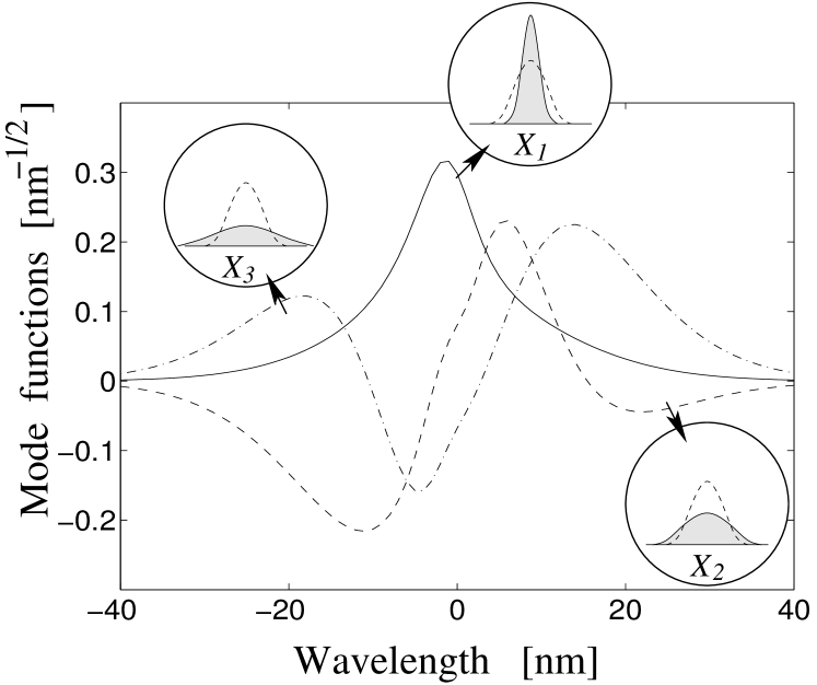
Figure 2: Mode functions for which the $V_{Xk,Xk^{\prime}}$ matrix of the pulse measured in SKKSL98 is diagonal. The insets show the fluctuations of the $X$-quadratures in comparison with the vacuum fluctuation (dashed line). In the main figure, the full line corresponds to the mode function $f_{1}$ with the squeezed quadrature, $V_{X1,X1}\approx 0.29$, dashed line to $f_{2}$ with $V_{X2,X2}\approx 1.39$, and the dash-dotted line to $f_{3}$ with $V_{X3,X3}\approx 2.69$.

III.5 Conclusion

We have seen that one mode description of a pulse is not sufficient to explain the experimental data of SKKSL98 , whereas a three mode description gives a good agreement with the measurements. However, we cannot conclude from this that the pulse does not contain more than three modes. In other modes the $P$-quadratures can be excited which do not influence the observed photon statistics. Also, the measurement noise was too high so that weak excitation of some additional modes might be undistinguished from the data noise backgraund.

It is interesting to compare our approach with that of Haus and Lai HausLai (see also Kaup90 ; Haus00 ; MK00 ). In their case the quantum field is decomposed into a “soliton” part and a “continuum” part. The soliton field is described by four operators $\Delta\hat{n}$, $\Delta\hat{\theta}$, $\Delta\hat{x}$, and $\Delta\hat{p}$, related to the soliton energy, phase, position, and velocity, respectively. As shown in App. F, these operators can be expressed by our quadrature operators of four modes, provided that the mode functions are properly selected. However, only two of these operators ($\Delta\hat{n}$ and $\Delta\hat{x}$) related to two our modes ($f_{1}$ and $f_{2}$) influence the photon statistics. Thus, confining ourselves to the four soliton operators of HausLai would not be sufficient to describe the observed phenomena. To apply the formalism of HausLai , one would have to work with the full set of the soliton and continuum operators.

IV Complete determination of the variance matrix

Even though one can obtain full information about the $X$-quadratures from the spectral correlations of photon numbers, one has no access to the variances $V_{Pk,Pk^{\prime}}$ and $V_{Xk,Pk^{\prime}}$. To get full information on the multimode Gaussian quantum state, one has to perform phase dependent measurements. Homodyne detection is one example of such a measurement; recently it was studied how to apply homodyne detection scheme to the quantum state reconstruction of a multimode optical field Reconstruc ; OWV97 . Because we confine ourselves to the Gaussian states, the task is easier than reconstruction of a general quantum state.

To find the variance matrix $V$, one can use the scheme of OWV97 with the local oscillator pulses shaped to the form of weighted combinations of the mode functions. It is very useful to subtract the coherent amplitude of the pulse by using a balanced Sagnac interferometer SH90 as in Fig. 3. Here, two counterpropagating identical squeezed pulses are interfering at a 50%/50% beam splitter. In one of the outputs of the beam splitter the pulses interfere constructively and form a bright pulse, which is then used to form the local oscillator. In the other output where the pulses interfere destructively, squeezed vacuum (or a more general field with zero mean amplitude) is formed. The squeezed vacuum pulse has the same quadrature variance matrix $V$ as each of the two counterpropagating pulses.

The bright pulse is shaped interferometrically so that its envelope has the form of different combinations of the mode functions $f_{k}(\omega)$. Such a pulse is then used as a local oscillator in a balanced homodyne detector. Thus, if the local oscillator is $f_{k}(\omega)$, one can obtain the value of $V_{Xk,Xk}$, whereas with the local oscillator $if_{k}(\omega)$ one can obtain $V_{Pk,Pk}$. Knowing these values and using the local oscillator pulse of the form $f_{k}(\omega)+f_{k^{\prime}}(\omega)$ one can obtain the value of $V_{Xk,Xk^{\prime}}$, by using the local oscillator form $i(f_{k}(\omega)+f_{k^{\prime}}(\omega))$ one can obtain the value of $V_{Pk,Pk^{\prime}}$, and by using the form $f_{k}(\omega)+if_{k^{\prime}}(\omega)$ one can obtain the value of $V_{Xm,Pm^{\prime}}$. Altogether, $N(2N+1)$ different forms of the local oscillator are sufficient to obtain all the $N(2N+1)$ independent elements of the variance matrix $V$. Let us note that to increase the precision of the measurements, one can increase the number of different phases of the local oscillator; a Maximum-Likelihood method for parameter estimations of a single mode Gaussian state using many phases has been discussed in DAriano .

Figure 3: Scheme to measure all the elements of the quadrature variance matrix. The Sagnac interferometer produces in one output squeezed vacuum and in the other output a bright pulse corresponding to one of the mode functions (say $f_{1}(\omega)$). The pulse shaping device transforms the bright pulse envelope into different combinations of the mode functions. Using the resulting bright pulse as a local oscillator in a balanced homodyne detector, one can reconstruct the quadrature variance matrix $V$.

Having found the variance matrix, one has all the information about the Gaussian state. Then we can immediately see, e.g., what is the maximum available squeezing of the state: it is the value corresponding to the minimum eigenvalue of $V$. Typically, this value will be smaller than the minimum diagonal element of $V$, which means that the optimum squeezing is shared among different modes. For example, there is a quadrature squeezing in the fundamental mode $f_{1}$ due to the Kerr effect (assuming mode functions as in App. F), but the $X_{1}$ quadrature is also correlated to the $X_{3}$ quadrature, because of the correlation between the pulse width and energy. Therefore, better squeezing can be expected to occur in a combination of the modes 1 and 3 than in the isolated mode 1. Thus, if the scheme is used to produce squeezing, the measurement scheme can serve as a tool for a selection of the optimum local oscillator.

One can also see how much are individual modes entangled with each other. To take full advantage of this knowledge one has to be able to separate individual modes from each other and distribute them among Alice, Bob, and other entanglement consumers. This is, however, a rather nontrivial task; in Sec. VII we will briefly mention a possible approach to its solution.

V Photon number squeezing via local oscillator modulation vs. spectral filtering

Let us assume that we want to prepare a pulse with the maximum photon number squeezing, i.e., the photon number fluctuates as little as possible. To quantify the photon number squeezing, one uses the Mandel $Q$-parameter Mandel defined as

$$Q=\frac{\langle\Delta n^{2}\rangle-\langle n\rangle}{\langle n\rangle},$$ (45)

where $n$ refers to the photon number of the entire pulse. This quantity is negative for sub-Poissonian field and positive for super-Poissonian fields. It was suggested in several works Friberg that spectral filtering of the pulse can lead to improvement of the photon number squeezing by blocking frequency bands with correlated photon fluctuations and letting through frequency bands with anticorrelated photon numbers. Here we show that a proper modulation of the coherent amplitude (playing the role of the local oscillator) leads to the optimum squeezing which cannot be overcome by the spectral filtering method.

V.1 Local oscillator modulation

Let us first assume that the quadrature variance matrix $V$ is fixed while we can modulate the mean values of the quadratures $\bar{X}_{n}$ and $\bar{P}_{n}$; this corresponds to the experimental situation as in Sec. IV and Fig. 3. The photon number variance is

$$\langle\Delta n^{2}\rangle=\sum_{k,l}\text{cov}\ (n_{k},n_{l}).$$ (46)

Assuming as in Sec. III.2 that the coherent amplitudes are much greater than the variance matrix elements, and that the mode functions are real (generalization to complex functions being straightforward), we can express the photon number variance as

$$\langle\Delta n^{2}\rangle=\sum_{m,n\leq N}\left(\bar{X}_{m}\bar{X}_{n}V_{Xm,Xn}\right.$$

$$\left.+2\bar{X}_{m}\bar{P}_{n}V_{Xm,Pn}+\bar{P}_{m}\bar{P}_{n}V_{Pm,Pn}\right).$$ (47)

The mean photon number is

$$\langle n\rangle=\sum_{k}\langle n_{k}\rangle=\frac{1}{2}\sum_{n\leq N}\left(\bar{X}_{n}^{2}+\bar{P}_{n}^{2}\right),$$ (48)

so that the $Q$-parameter of Eq. (45) can be written, after some algebra, as

$$Q=2\sum_{m,n\leq N}\left[\tilde{X}_{m}\left(V_{Xm,Xn}-\frac{\delta_{mn}}{2}\right)\tilde{X}_{n}\right.$$

$$\left.+2\tilde{X}_{m}V_{Xm,Pn}\tilde{P}_{n}+\tilde{P}_{m}\left(V_{Pm,Pn}-\frac{\delta_{mn}}{2}\right)\tilde{P}_{n}\right],$$ (49)

where

$$\tilde{X}_{m}\equiv\frac{\bar{X}_{m}}{\sqrt{\sum_{n\leq N}\left(\bar{X}_{n}^{2}+\bar{P}_{n}^{2}\right)}},$$ (50)

$$\tilde{P}_{m}\equiv\frac{\bar{P}_{m}}{\sqrt{\sum_{n\leq N}\left(\bar{X}_{n}^{2}+\bar{P}_{n}^{2}\right)}}.$$ (51)

Thus the $Q$-parameter can be expressed in the matrix multiplication form as

$$Q=2\left(\tilde{X}^{T},\tilde{P}^{T}\right)\left(\begin{array}[]{cc}V_{XX}&V_{XP}\\ V_{PX}&V_{PP}\end{array}\right)\left(\begin{array}[]{c}\tilde{X}\\ \tilde{P}\end{array}\right)-1,$$ (56)

where $\tilde{X}$ and $\tilde{P}$ are column vectors with the $\tilde{X}_{m}$ and $\tilde{P}_{m}$ elements, and $V_{XX}$, $V_{XP}$, and $V_{PP}$ are the corresponding submatrices of the variance matrix $V$. The variance matrix is multiplied from the left and from the right with a unit vector, so that the $Q$-parameter is limited by

$$2\left(V^{\text{(min)}}-\frac{1}{2}\right)\leq Q\leq 2\left(V^{\text{(max)}}-\frac{1}{2}\right),$$ (57)

where $V^{\text{(min)}}$ is the minimum eigenvalue of the variance matrix $V$ and $V^{\text{(max)}}$ is its maximum eigenvalue. The minimum value of $Q$ is reached if the vector of mean values of $X$ and $P$ is the eigenvector of $V$ corresponding to its minimum eigenvalue. Setting the components of this vector is possible using the scheme of Fig. 3.

V.2 Spectral filtering

Let us assume a spectral filtering function $0\leq c(\omega)\leq 1$: the frequency component is completely transmitted if $c(\omega)=1$ and it is completely blocked if $c(\omega)=0$. This function transforms the mean quadratures and variances as

$$\bar{x}_{k}^{f} = c(\omega_{k})\bar{x}_{k},$$ (58)

$$\bar{p}_{k}^{f} = c(\omega_{k})\bar{p}_{k},$$ (59)

$$V^{\prime f}_{xk,xl} = c(\omega_{k})V^{\prime}_{xk,xl}c(\omega_{l})+\frac{\delta_{kl}}{2}\left[1-c^{2}(\omega_{k})\right],$$ (60)

$$V^{\prime f}_{pk,pl} = c(\omega_{k})V^{\prime}_{pk,pl}c(\omega_{l})+\frac{\delta_{kl}}{2}\left[1-c^{2}(\omega_{k})\right],$$ (61)

$$V^{\prime f}_{xk,pl} = c(\omega_{k})V^{\prime}_{xk,pl}c(\omega_{l}).$$ (62)

The $\delta_{kl}$ terms in Eqs. (60) and (61) follow from the quantum mechanical nature of the quadratures: partially blocking a frequency component means that the corresponding field is mixed with vacuum.

Eqs. (58)–(62) can be used to determine $\langle\Delta n^{2}\rangle$ and $\langle n\rangle$ as in the preceding subsection, and thus to find the $Q$-parameter of the filtered field. After a straightforward algebra, one can express the new $Q$-parameter as

$$Q^{f}=2\sum_{m,n\leq N}\left[\tilde{X}^{f}_{m}\left(V_{Xm,Xn}-\frac{\delta_{mn}}{2}\right)\tilde{X}^{f}_{n}\right.$$

$$\left.+2\tilde{X}^{f}_{m}V_{Xm,Pn}\tilde{P}^{f}_{n}+\tilde{P}^{f}_{m}\left(V_{Pm,Pn}-\frac{\delta_{mn}}{2}\right)\tilde{P}^{f}_{n}\right],$$ (63)

where

$$\tilde{X}^{f}_{m}=\frac{\sum_{n\leq N}c_{mn}\bar{X}_{n}}{\sqrt{\sum_{n,n^{\prime}\leq N}c_{nn^{\prime}}\left(\bar{X}_{n}\bar{X}_{n^{\prime}}+\bar{P}_{n}\bar{P}_{n^{\prime}}\right)}},$$ (64)

$$\tilde{P}^{f}_{m}=\frac{\sum_{n\leq N}c_{mn}\bar{P}_{n}}{\sqrt{\sum_{n,n^{\prime}\leq N}c_{nn^{\prime}}\left(\bar{X}_{n}\bar{X}_{n^{\prime}}+\bar{P}_{n}\bar{P}_{n^{\prime}}\right)}},$$ (65)

with

$$c_{nn^{\prime}}=\int c^{2}(\omega)f_{n}(\omega)f_{n^{\prime}}(\omega)d\omega.$$ (66)

Again, the $Q$-parameter is calculated as a matrix product of the variance $V$ multiplied from the left and from the right by a vector. This time, however, the vector is not of the unit length, so that $Q^{f}$ is limited by

$$2A^{2}\left(V^{\text{(min)}}-\frac{1}{2}\right)\leq Q^{f}\leq 2A^{2}\left(V^{\text{(max)}}-\frac{1}{2}\right),$$ (67)

where $A^{2}$ is the square of the magnitude of the multiplying vector,

$$A^{2}=\sum_{n\leq N}\left(\tilde{X}^{f2}_{n}+\tilde{P}^{f2}_{n}\right).$$ (68)

To show that $Q^{f}$ can never be smaller than the minimum value achievable by local oscillator modulation, it is enough to show that $A^{2}\leq 1$, i.e., that the magnitude of the multiplying vector is not bigger than one. Proof of this inequality is shown in Appendix D.

V.3 Conclusion

We can see that no spectral filtering can improve the photon number squeezing below the minimum eigenvalue of the quadrature variance matrix, which is available via the local oscillator modulation approach. Let us stress that our method of finding the optimum local oscillator function is very simple and straightforward since it is based on linear algebra. It was suggested recently to use an adaptive algorithm to optimize the pulse shape for achieving optimum photon number squeezing Takeoka . In this method, the optimum was reached after 20 000 iterations. In our case, provided that the pulse is sufficiently well described by $N=5$ modes, $N(2N+1)=55$ iterations is enough.

VI Selection of appropriate mode functions

So far it was assumed that the set of mode functions was given and the question was about the statistics of the corresponding quadratures. But how should these mode functions be selected?

In principle, any orthogonal set of mode functions can be used for description of the pulse statistics. However, since the aim is to reduce the number of quantum variables necessary to describe the pulse, the functions should be carefully chosen. One possibility is to start from theory and assume some particular shape of the pulse - e.g., a hyperbolic secant soliton and to construct the orthogonal set from the typical perturbations. An example is given in App. F, Eqs. (111)–(114) where relationship to the soliton quantum fluctuations approach by Haus and Lai HausLai is discussed.

Another approach does not assume any particular mode function form and is related directly to the experiment. It is useful to assume that only one mode has a nonzero coherent amplitude and a very small number of modes have quadrature fluctuations substantially different from the vacuum values. To find the optimum set of mode functions, one can use the following procedure.

1. Select $f_{1}(\omega)$ as the measured classical envelope of the pulse (see App. E).

2. Determine the minimum value of variance to be still considered as different from vacuum.

3. Construct a temporary set of orthogonal functions $f^{\text{(temp)}}_{k}$, $k=1\dots N^{\prime}$ with $f^{\text{(temp)}}_{1}=f_{1}$ chosen in 1. The size $N^{\prime}$ of the temporary set should reasonably correspond to the experimental conditions.

4. Perform the measurement of the $2N^{\prime}\times 2N^{\prime}$ variance matrix $V^{(1)}$ with the temporary set of mode functions.

5. Construct the reduced matrix $V^{(2)}$ from $V^{(1)}$ by excluding rows and columns referring to quadratures of mode 1. Let indexes $1\dots N^{\prime}-1$ correspond to the $X$ quadratures, and indexes $N^{\prime}\dots N^{\prime}-2$ correspond to the $P$ quadratures.

6. Diagonalize $V^{(2)}$ to get $\tilde{V}^{(2)}=WV^{(2)}W^{T}$ with $W$ an orthogonal matrix. Let us choose $W$ such that $\tilde{V}^{(2)}_{11}$ is the largest element of $\tilde{V}^{(2)}$; $\tilde{V}^{(2)}_{11}=\sum_{k,l}W_{1k}W_{1l}V^{(2)}_{k,l}$.

7. The function $f_{2}$ is constructed as

   $$f_{2}=\sum_{k=1}^{N^{\prime}-1}\left(W_{1k}+iW_{1k+N^{\prime}-1}\right)f^{\text{(temp)}}_{(k+1)}.$$ (69)

   It can be checked that the variance of the $X$ quadrature corresponding to this mode function is $\langle\hat{X}_{2}^{2}\rangle=\tilde{V}^{(2)}_{11}$.

8. A new temporary set of $N^{\prime}-2$ mode functions is constructed from the old one as an orthogonal complement to $f_{1}$ and $f_{2}$. By means of the transformation connecting the new temporary set of mode functions to the initial one, calculate the corresponding variance matrix. Construct reduced matrix $V^{(3)}$ by excluding rows and columns referring to quadratures of modes 1 and 2. Diagonalize $V^{(3)}$ and find mode function $f_{3}$ in the same way as in 6 and 7. Note that the variances of the quadratures of mode 3 are smaller than the variance $\langle\hat{X}_{2}^{2}\rangle$.

9. Repeat this procedure of redefining the temporary mode set, transforming and diagonalizing the variance matrix, and defining a new mode function. After each repetition, the maximum variance of the $(n+1)$st mode is smaller than the maximum variance of the $n$th mode. If for some $n=N$ the variance of mode $n+1$ is sufficiently close to $1/2$ (as defined in item 2), the quantum state of the $(n+1)$st mode is indistinguishable from vacuum. The pulse can be described with the given precision as an $N$-mode object.

Let us note that the procedure of redefining the temporary mode set and rediagonalizing the reduced variance matrix each time when a new mode function is constructed is necessary. It is not possible, as one might be tempted, to find a set of mode functions simply by diagonalizing the measured variance matrix, since the SO(2$N$) transformation corresponding to diagonalization is generally not a canonical transformation (see, e.g. SMD94 for more details). On the other hand, in the special case of pure Gaussian states which are specified by $N(N+1)$ real parameters one can find a set of uncorrelated modes. In this case our procedure would be terminated after the first diagonalization. The diagonalization of pure Gaussian multimode states into uncorrelated modes has recently been studied in Bennink .

The procedure of operational construction of mode functions as described above is, of course, not the only possible. It is, however, very useful for finding the minimum subspace of mode functions sufficient for the pulse description. Other sets of mode functions can be selected such that the variance matrix takes some special shape, e.g., some of the “canonical” forms studied in SMD94 .

VII Separation of modes

It may be very useful to separate individual nonmonochromatic modes which form the pulse. The possibility of obtaining nonclassical correlations of optical pulses by partitioning the pulse in the spectral region was suggested in SKW00 . Similarly as with spectral filtering, this approach is not necessarily the optimum one for obtaining maximum entanglement from the source.

The basic idea for obtaining the optimum separation is to send different (nonmonochromatic) modes into different channels by using a special unitary transformation among them. It was shown in Reck that any discrete unitary operator can be constructed interferometrically. For this purpose we suggest to apply a scheme as in Fig. 4. In the first step one decomposes the pulse into quasimonochromatic components. The frequencies of these components are then shifted by means of acusto-optical modulators (AOMs) so that each channel has the same central frequency. The channels then interfere on a 2$N$-port consisting of beam splitters and mirrors. By a proper choice of the 2$N$-port parameters one can manage that most of a pulse in the $f_{k}(\omega)$ mode leaves the 2$N$-port in the $k$th output channel.

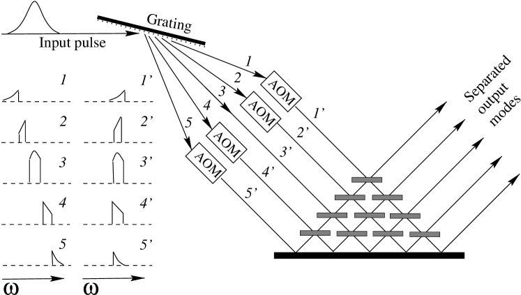
Figure 4: Scheme to separate individual nonmonochromatic modes. The pulse is first decomposed on a grating into quasimonochromatic channels. The frequency of each channel is then shifted by means of an AOM to the central frequency of the pulse. The resulting modes (with the same central frequency) then interfere on a 2$N$-port.

One can also optimize the 2$N$-port parameters to prepare a set of optimally entangled $K$ modes (multipartite entanglement), sent to different channels. This would be a generalization of the proposal of SKW00 for partitioning soliton pulses to generate entangled states.

Let us note that the spectral filtering of solitons used to produce photon number squeezing Friberg is a special kind of mode separation. However, as shown in Sec. V, in this case the separation is not optimized with respect to all relevant degrees of freedom. Therefore, better results can be expected in our general approach.

VIII Discussion and conclusion

To summarize our results we can state that:

$(i)$ For a complete description of the experimental results measured on optical solitons it appears that a very small number of nonmonochromatic modes is enough. The results cannot be described by means of a single-mode field, but already three nonmonochromatic modes were sufficient to reproduce the experimental data of SKKSL98 . With our approach it is easy to interpret the “butterfly” pattern of the measured photon covariances: three different non-monochromatic modes overlap and contribute with their fluctuating in-phase quadratures to the photon statistics (see Fig. 2).

$(ii)$ Provided that the pulses are Gaussian (which seems to be a relevant assumption for most of the experimental situations), a complete quantum description of the pulse can be done by means of a multimode variance matrix. The elements of this matrix can be determined by means of homodyne detection with specially shaped local oscillator pulses.

$(iii)$ Concrete form of the mode functions is a matter of choice. If the aim is to find the smallest number of modes, an operational method for constructing the mode functions is provided. In this case the first mode contains the coherent amplitude, whereas the rest of the modes have zero mean fields and their field variances decrease with increasing mode index. By selecting the minimum set of modes, one can substantially reduce the number of parameters necessary for a complete description of the physical situation.

$(iv)$ Knowledge of the mode structure of the pulse and of the corresponding quantum state will be very useful for quantum information purposes: one can select the optimum shape of the local oscillator pulse to detect maximum squeezing or entanglement. This optimum finding is very straightforward and much faster than adaptive algorithms as in Takeoka . One can also relatively easily study the influence of the medium on the propagated pulses and on the quantum information they carry. By measurement of the multimode quantum state of the input and output pulses we can find the von Neumann entropy of the states. This would enable us to tell whether the observed pulse deformation corresponds most probably to a unitary evolution or rather to decay and dephasing, possibly caused by an eavesdropper.

$(v)$ In principle, one can also separate individual modes to match the requirements of the pulse user, e.g., to prepare a single mode maximally squeezed field, or to extract a maximally entangled two-mode field, etc.

$(vi)$ The pulse separation is generalization of spectral filtering which has also been used for observation of photon number squeezing Friberg . We have shown that spectral filtering can never beat the coherent amplitude modulation approach in achieving better photon number squeezing. In our approach, we can understand why spectral filtering can help with squeezing, but we can also see its limitations.

$(vii)$ Our approach of multimode description of solitons is different from the approach by Haus and Lai HausLai (see App. F for more details). The formalism of HausLai was developed to solve an idealized quantum soliton equation and to study the soliton dynamics. Its essential feature is the decomposition of the field into the “soliton” and “continuum” part, where the soliton field is completely described by four operators. Our approach ignores the dynamics (which is rather complicated in real life), focusing on the phenomenological description of the pulse. The four soliton operators of HausLai can be expressed by means of our quadrature operators, but they alone appear to be insufficient for description of the observed phenomena. It is necessary to work with the complete set of “soliton” and “continuum” operators if one wishes to describe the observed pulses using the formalism of HausLai .

Appendix A Simplified calculation of transformed mean quadratures and variances for few excited modes

Let us assume that only the first $N$ modes of the $\hat{b}_{k}$ system are occupied, while the rest is in vacuum, $|0\rangle_{k}$ for $k>N$. The quadrature means and variances are thus

$$\overline{\mu}_{k}=0\quad{\rm for}\ k>N,$$ (70)

and

$$V_{\mu k,\mu k} = \frac{1}{2}\quad\text{for}\ k>N,$$

$$V_{\mu k,\mu^{\prime}k^{\prime}} = 0\quad\text{for}\ \mu\neq\mu^{\prime}$$ (71)

$$\text{and}\ (k>N\ \text{or}\ k^{\prime}>N).$$

The transformations (27) and (29) can then be written as

$$\bar{\xi}_{j}=\tilde{\sum_{\mu,k}}Z^{\mu\xi}_{kj}\bar{\mu}_{k},$$ (72)

and

$$V^{\prime}_{\xi j,\xi^{\prime}j^{\prime}}=\tilde{\sum_{\mu,k}}\tilde{\sum_{\mu,k^{\prime}}}Z^{\mu\xi}_{kj}\ V_{\mu k,\mu^{\prime}k^{\prime}}\ Z^{\mu^{\prime}\xi^{\prime}}_{k^{\prime}j^{\prime}}$$

$$+\frac{1}{2}\sum_{\mu}\sum_{k>N}Z^{\mu\xi}_{kj}\ Z^{\mu,\xi^{\prime}}_{kj^{\prime}}\$$ (73)

$$\!=\!\tilde{\sum_{\mu,\mu^{\prime}k,k^{\prime}}}\!\left[Z^{\mu\xi}_{kj}\left(V_{\mu k,\mu^{\prime}k^{\prime}}\!-\!\frac{\delta_{\mu\mu^{\prime}}\delta_{kk^{\prime}}}{2}\right)Z^{\mu^{\prime}\xi^{\prime}}_{k^{\prime}j^{\prime}}\right]\!+\!\frac{\delta_{\xi\xi^{\prime}}\delta_{jj^{\prime}}}{2}$$

(74)

with

$$\tilde{\sum_{\mu,k}}\equiv\sum_{\mu=X,P}\sum_{k=1}^{N}.$$ (75)

To get (74) from (73), the orthogonality and completeness relation (20) was used. As a special case, let us consider the variance matrix elements $V^{\prime}_{xj,xj^{\prime}}$ when the mode functions $f_{k}(\omega)$ are real, as in Sec. III.2. Eq. (74) then becomes

$$V^{\prime}_{xj,xj^{\prime}}=\frac{\delta_{jj^{\prime}}}{2}$$

$$+\!\sum_{k,k^{\prime}\leq N}f_{k}(\omega_{j})f_{k^{\prime}}(\omega_{j^{\prime}})\Delta\omega\left(V_{Xk,Xk^{\prime}}\!-\!\frac{\delta_{kk^{\prime}}}{2}\right).$$ (76)

Appendix B Quadrature moments of multimode Gaussian states

An $N$-mode Gaussian state with mean quadratures $\overline{\mu}$ and variance matrix $V$ has the Wigner function $W(\mu)$,

$$W(\mu)\!=\!\frac{1}{(2\pi)^{N}\!\sqrt{{\rm det}\ V}}\exp\left[-\frac{\left(\mu\!-\!\overline{\mu}\right)^{T}\!V^{-1}\!\left(\mu\!-\!\overline{\mu}\right)}{2}\right],$$ (77)

where $V^{-1}$ is the matrix inversion of $V$. Thus, a Gaussian state is fully determined by 2$N^{2}$ $+$ 3$N$ real parameters (2$N$ mean quadratures plus $N(2N+1)$ independent elements of the symmetric matrix $V$).

Generally, a quadrature moment $\langle\hat{\mu}_{k}^{n}\rangle$ can be calculated as the integral of the Wigner function

$$\langle\hat{\mu}_{k}^{n}\rangle=\int\dots\int\mu_{k}^{n}W(\mu)dX_{1}\dots dP_{N}.$$ (78)

The symmetrical two-variable moments $\frac{1}{2}\left\langle\left\{\hat{\mu}_{k},\hat{\mu}^{\prime}_{k^{\prime}}\right\}\right\rangle$ and $\frac{1}{2}\left\langle\left\{\hat{\mu}_{k}^{2},\hat{\mu}_{k^{\prime}}^{2}\right\}\right\rangle$ can be calculated as

$$\frac{1}{2}\left\langle\left\{\hat{\mu}_{k},\hat{\mu}^{\prime}_{k^{\prime}}\right\}\right\rangle=\int\dots\int\mu_{k}\mu^{\prime}_{k^{\prime}}W(\mu)dX_{1}\dots dP_{N}$$ (79)

and

$$\frac{1}{2}\!\left\langle\left\{\hat{\mu}_{k}^{2},\hat{\mu}_{k^{\prime}}^{\prime 2}\right\}\right\rangle=\int\dots\int\mu_{k}^{2}\mu_{k^{\prime}}^{\prime 2}W(\mu)dX_{1}\dots dP_{N}$$

$$-\frac{1}{2}\tilde{\delta}_{\mu k,\mu^{\prime}k^{\prime}},\!$$ (80)

where $\tilde{\delta}_{\mu k,\mu^{\prime}k^{\prime}}$ $\equiv$ 0 if $\mu_{k}$ and $\mu^{\prime}_{k^{\prime}}$ commute with each other, and $\tilde{\delta}_{\mu k,\mu^{\prime}k^{\prime}}$ $\equiv$ 1 if $\mu_{k}$ and $\mu^{\prime}_{k^{\prime}}$ are conjugate variables. Using Eq. (77) one can analytically evaluate the integrals and express the quadrature moments by means of the parameters $\overline{\mu}_{k}$ and $V^{\prime}_{\mu k,\mu^{\prime}k^{\prime}}$. We obtain

$$\langle\hat{\mu}_{k}\rangle = \overline{\mu}_{k},$$ (81)

$$\langle\hat{\mu}_{k}^{2}\rangle = \overline{\mu}_{k}^{2}+V_{\mu k,\mu k},$$ (82)

$$\langle\hat{\mu}_{k}^{3}\rangle = \overline{\mu}_{k}^{3}+3\overline{\mu}_{k}V_{\mu k,\mu k},$$ (83)

$$\langle\hat{\mu}_{k}^{4}\rangle = \overline{\mu}_{k}^{4}+6\overline{\mu}_{k}^{2}V_{\mu k,\mu k}+3V_{\mu k,\mu k}^{2},$$ (84)

$$\frac{1}{2}\left\langle\left\{\hat{\mu}_{k},\hat{\mu}^{\prime}_{k^{\prime}}\right\}\right\rangle = \bar{\mu}_{k}\bar{\mu}_{k^{\prime}}+V_{\mu k,\mu^{\prime}k^{\prime}},$$ (85)

and

$$\frac{1}{2}\left\langle\left\{\hat{\mu}_{k}^{2},\hat{\mu}_{k^{\prime}}^{\prime 2}\right\}\right\rangle=\bar{\mu_{k}}^{2}\bar{\mu}_{k^{\prime}}^{\prime 2}+\bar{\mu_{k}}^{2}V_{\mu^{\prime}k^{\prime},\mu^{\prime}k^{\prime}}+\bar{\mu}_{k^{\prime}}^{\prime 2}V_{\mu k,\mu k}$$

$$+V_{\mu k,\mu k}V_{\mu^{\prime}k^{\prime},\mu^{\prime}k^{\prime}}+4\bar{\mu_{k}}\bar{\mu^{\prime}}_{k^{\prime}}V_{\mu k,\mu^{\prime}k^{\prime}}$$

$$+2V_{\mu k,\mu^{\prime}k^{\prime}}^{2}-\frac{1}{2}\tilde{\delta}_{\mu k,\mu^{\prime}k^{\prime}}.$$ (86)

Note that although (81), (82), and (85) are generally valid for all states, the equalities (83), (84), and (86) only hold for Gaussian states. Corresponding expressions can be found also for the moments of the quadratures $\xi(\omega)$.

Appendix C Photon statistics in different frequency channels of a single nonmonochromatic mode

Let us assume a nonmonochromatic mode defined by the discrete function $f(\omega_{k})$, $k=1\dots N$, $\sum_{k=1}^{N}|f(\omega_{k})|^{2}$ $=$ 1. Let the state of this mode be Gaussian. We are interested in the photon number correlations between different frequency channels.

Theorem: All non-zero elements of a multi-mode photon correlation matrix of an effectively single-mode Gaussian state have the same sign. They are negative (positive) iff the single-mode state is sub(super)-Poissonian.

Proof: The mode function $f(\omega_{k})$ defines the first row of the unitary transformation matrix $U$. Let the parameters of the single-mode Gaussian state be $\bar{X}$, $\bar{P}$, $V_{XX}$, $V_{PP}$, and $V_{XP}$. The multi-mode parameters $\bar{x}_{k}$, $\bar{p}_{k}$, $V_{xk,xl}$, $V_{xk,pl}$, etc., can be calculated by means of the simplified summation as in (72) and (74). The sign of the off diagonal element of the correlation matrix (36) is determined by the sign of the covariance (33). After some algebra with applying Eqs. (72), (74), and (34) we arrive at

$${\rm cov}\ (n_{k},n_{l})=|f(\omega_{k})|^{2}|f(\omega_{l})|^{2}$$

$$\times\left[\bar{X}^{2}\left(V_{XX}\!-\!\frac{1}{2}\right)+\ 2\bar{X}\bar{P}V_{XP}+\bar{P}^{2}\left(V_{PP}\!-\!\frac{1}{2}\right)\right.$$

$$\left.+\frac{1}{2}\left(V_{XX}\!-\!\frac{1}{2}\right)^{2}+V^{\prime 2}_{XP}+\frac{1}{2}\left(V_{PP}\!-\!\frac{1}{2}\right)^{2}\right].$$ (87)

Thus, we can see that the sign of the non-zero elements does not depend on the arguments $\omega_{k}$ and $\omega_{l}$, but is fully determined by the expression in the square brackets. If we denote the photon number in the single mode by $\hat{n}$, we find that the quantity $\Delta n^{2}-\langle n\rangle$ is equal to the expression in the square brackets. This quantity is negative for sub-Poissonian states and positive for super-Poissonian states by definition, QED.

Appendix D Proof that the magnitude of the spectral-filtering quadrature vector is less than 1

Showing that

$$A^{2}=\sum_{n\leq N}\left(\tilde{X}^{f2}_{n}+\tilde{P}^{f2}_{n}\right)\leq 1$$ (88)

is equivalent to showing that

$$\sum_{k,l,n\leq N}c_{kn}c_{ln}\left(\bar{X}_{k}\bar{X}_{l}+\bar{P}_{k}\bar{P}_{l}\right)$$

$$\leq\sum_{k,l\leq N}c_{kl}(\bar{X}_{k}\bar{X}_{l}+\bar{P}_{k}\bar{P}_{l}),$$ (89)

which follows directly from the definitions of $\tilde{X}^{f}$ and $\tilde{P}^{f}$, Eqs. (64), (65). To violate Eq. (89), it would be necessary to have some vector $Y$ such that

$$Y^{T}\underline{c}^{2}Y>Y^{T}\underline{c}Y,$$ (90)

where $\underline{c}$ is a matrix with the elements $c_{kl}$. Eq. (90) could only be valid if there exists some eigenvalue $c_{\lambda}$ of $\underline{c}$ such that $c_{\lambda}>1$. Let us assume that such an eigenvalue does exist. Let $u_{k}$ be the elements of the corresponding eigenvector, i.e.,

$$\sum_{l\leq N}c_{kl}u_{l}=c_{\lambda}u_{k},$$ (91)

i.e.,

$$\sum_{l\leq N}u_{l}\int c^{2}(\omega)f_{k}(\omega)f_{l}(\omega)d\omega=c_{\lambda}u_{k}.$$ (92)

Let us define a function $q(\omega)$ as

$$q(\omega)=\sum_{l\leq N}u_{l}f_{l}(\omega).$$ (93)

Since $u_{k}=\int q(\omega)f_{k}(\omega)d\omega$, one has

$$\int c^{2}(\omega)q(\omega)f_{k}(\omega)d\omega=c_{\lambda}\int q(\omega)f_{k}(\omega)d\omega,$$ (94)

i.e.,

$$\left|\int c^{2}(\omega)q(\omega)f_{k}(\omega)d\omega\right|>\left|\int q(\omega)f_{k}(\omega)d\omega\right|,$$ (95)

which cannot happen for any function $q(\omega)$ since $|c^{2}(\omega)|\leq 1$. Thus, $A^{2}\leq 1$, QED.

Appendix E Elimination of coherent amplitudes of a multi-mode Gaussian state

Let us assume that $N$ modes of the $b$-system are excited and the rest is in vacuum. Then, one can redefine the $N$ modes such that only one of them (say mode $\hat{b}_{1}$) has nonzero values of $\bar{X}_{1}$, $\bar{P}_{1}$, whereas $\bar{X}_{m}$ $=$ 0, $\bar{P}_{m}$ $=$ 0 for $m$ $>$ 1 (the variance matrix elements corresponding to these modes are, however, generally non-zero).

Proof: Define $\beta_{m}$ $\equiv$ $2^{-1/2}(\bar{X}_{m}+i\bar{P}_{m})$ $=$ $\langle\hat{b}_{m}\rangle$, $m$ $=$ $1\dots N$. Let $f_{m}$ be the mode functions normalized such that $(f_{m},f_{m^{\prime}})$ $=$ $\delta_{mm^{\prime}}$, where the bracket denotes the scalar product. Let us define a new mode function $g_{1}$ as $g_{1}$ $\equiv$ $A\sum_{m=1}^{N}\beta^{*}_{m}f_{m}$ and a corresponding annihilation operator $\hat{h}_{1}$ $\equiv$ $A\sum_{m=1}^{N}\beta^{*}_{m}\hat{b}_{m}$, where $A$ $=$ $\left(\sum_{m=1}^{N}|\beta_{m}|^{2}\right)^{-1/2}$. Then $\langle\hat{h}_{1}\rangle$ $=$ $\sqrt{\sum_{m=1}^{N}|\beta_{m}|^{2}}$. Let us define mode functions $g_{2}\dots g_{N}$ as linear combinations of $f_{1}\dots f_{N}$ by some orthogonalization procedure, i.e., $g_{m}$ $=$ $\sum_{m^{\prime}=1}^{N}G_{mm^{\prime}}f_{m^{\prime}}$, $m=2\dots N$ such that $(g_{m},g_{m^{\prime}})$ $=$ $\delta_{mm^{\prime}}$, $m=1\dots N$. In particular,

$$(g_{1},g_{m})=A\sum_{l=1}^{N}\beta_{l}G_{ml}=0$$ (96)

for $m>1$. The annihilation operators corresponding to the $g$-modes are $\hat{h}_{m}$ $\equiv$ $\sum_{m^{\prime}=1}^{N}G_{mm^{\prime}}\hat{b}_{m^{\prime}}$, and their mean values are $\langle\hat{h}_{m}\rangle$ $=$ $\sum_{m^{\prime}=1}^{N}G_{mm^{\prime}}\langle\hat{b}_{m^{\prime}}\rangle$ $=$ $\sum_{m^{\prime}=1}^{N}G_{mm^{\prime}}\beta_{m^{\prime}}$ $=$ 0 according to (96). Thus, in the new system of modes only the first one has a non-zero coherent amplitude, QED.

Appendix F Relationship to the soliton perturbation approach by Haus and Lai

In HausLai (see also Haus00 ; MK00 ) it is suggested to describe the quantum fluctuations of the Nonlinear Schrödinger equation (NSE) soliton by writing

$$\hat{a}(x,t)=a_{o}(x,t)+\Delta\hat{a}(x,t),$$ (97)

where $a_{o}(x)$ is the unperturbed solution of the NSE of the hyperbolic secant form, and

$$\Delta\hat{a}=\Delta\hat{a}_{\text{sol}}+\Delta\hat{a}_{\text{cont}}$$ (98)

is the quantum perturbation part with $\Delta\hat{a}_{\text{sol}}$ describing fluctuations of the soliton degrees of freedom, while $\Delta\hat{a}_{\text{cont}}$ corresponds to field fluctuations not contained in the soliton solution and thus belonging to the continuum. The soliton fluctuations are expressed by means of four operators $\Delta\hat{n}$, $\Delta\hat{\theta}$, $\Delta\hat{x}$, and $\Delta\hat{p}$ as

$$\Delta\hat{a}_{\text{sol}}=\left[\Delta\hat{n}(t)f_{n}(x)+\Delta\hat{\theta}(t)f_{\theta}(x)\right.$$

$$\left.+\Delta\hat{x}(t)f_{x}(x)+n_{o}\Delta\hat{p}(t)f_{p}(x)\right]\times\exp\left(i\frac{KA_{o}^{2}}{2}t\right),$$ (99)

where the functions $f_{n}$, $f_{\theta}$, $f_{x}$, and $f_{p}$ are derivatives of the soliton function

$$a_{o}(x,t)=A_{o}\exp\left[i\left(\frac{KA_{o}^{2}}{2}t-\frac{C}{2}p_{o}^{2}t+p_{o}x+\theta_{o}\right)\right]$$

$$\times\text{sech}\left(\frac{x-x_{o}-Cp_{o}t}{\xi}\right)$$ (100)

with respect to the parameters $n_{o}(=2\xi|A_{o}|^{2})$, $p_{o}$, $\theta_{o}$, and $x_{o}$. In these equations the value $n_{o}$ is the mean photon number of the pulse, $\xi$ is the soliton width, $p_{o}$ and $x_{o}$ refer to the carrier frequency and soliton center position, respectively. The value $K$ is related to the Kerr nonlinearity and $C$ to the medium dispersion. To find the values of the operators from measured data, one introduces adjoint functions $\underline{f}_{n}$, $\underline{f}_{\theta}$, $\underline{f}_{x}$, and $\underline{f}_{p}$ with the property

$$\text{Re}\ \left[\int\underline{f}^{*}_{k}(x)f_{l}(x)dx\right]=\delta_{kl}$$ (101)

with $k,l=n,\theta,x,p$ (note that $f_{k}$ themselves do not form an orthogonal set; explicit form of functions $f_{k}$ and $\underline{f}_{k}$ can be found in Haus00 ). Writing $\Delta\hat{a}$ as a sum of hermitian operators $\Delta\hat{a}=\Delta\hat{a}^{(1)}+i\Delta\hat{a}^{(2)}$ one finds that

$$\Delta\hat{n} = \int\underline{f}_{n}^{*}(x)\Delta\hat{a}^{(1)}(x)dx,$$ (102)

$$\Delta\hat{\theta} = i\int\underline{f}_{\theta}^{*}(x)\Delta\hat{a}^{(2)}(x)dx,$$ (103)

$$\Delta\hat{x} = \int\underline{f}_{x}^{*}(x)\Delta\hat{a}^{(1)}(x)dx,$$ (104)

$$\Delta\hat{p} = i\frac{1}{n_{o}}\int\underline{f}_{p}^{*}(x)\Delta\hat{a}^{(2)}(x)dx.$$ (105)

The relationship of this approach to our scheme can be easily examined if one assumes the first four mode functions $f_{k}(\omega)$ in the form

$$f_{1}(\omega) = \frac{1}{\sqrt{2\omega_{o}}}\text{sech}\frac{\omega}{\omega_{o}},$$ (107)

$$f_{2}(\omega) = \sqrt{\frac{3}{2\omega_{o}}}\text{tanh}\frac{\omega}{\omega_{o}}\text{sech}\frac{\omega}{\omega_{o}},$$ (108)

$$f_{3}(\omega) = \frac{1}{\sqrt{\frac{1}{3}+\frac{\pi^{2}}{9}}}\frac{1}{\sqrt{2\omega_{o}}}$$ (109)

$$\times \left(2\frac{\omega}{\omega_{o}}\text{tanh}\frac{\omega}{\omega_{o}}\text{sech}\frac{\omega}{\omega_{o}}-\text{sech}\frac{\omega}{\omega_{o}}\right),$$

$$f_{4}(\omega) = i\frac{\sqrt{3}}{\sqrt{\frac{\pi^{2}}{9}-1}}\frac{1}{\sqrt{2\omega_{o}}}$$ (110)

$$\times \left(\text{tanh}\frac{\omega}{\omega_{o}}\text{sech}\frac{\omega}{\omega_{o}}-\frac{2}{3}\frac{\omega}{\omega_{o}}\text{sech}\frac{\omega}{\omega_{o}}\right).$$

These functions were obtained by an orthogonalization procedure from the Fourier transformed functions $f_{n,\theta,x,p}$ with $\omega_{o}=2c/(\pi\xi)$. With this choice of the mode functions one finds that the soliton perturbation operators can be expressed by means of the quadratures $\hat{X}_{1}$, $\hat{X}_{2}$, $\hat{P}_{1}$, $\hat{P}_{2}$, $\hat{P}_{3}$, and $\hat{P}_{4}$ as

$$\Delta\hat{n} = \sqrt{2n_{o}}\hat{X}_{1},$$ (111)

$$\Delta\hat{\theta} = \frac{1}{\sqrt{2n_{o}}}\hat{P}_{1}+\frac{\sqrt{\frac{1}{3}+\frac{\pi^{2}}{9}}}{\sqrt{2n_{o}}}\hat{P}_{3},$$ (112)

$$\Delta\hat{x} = \frac{2c}{\sqrt{6n_{o}}\omega_{o}}\hat{X}_{2},$$ (113)

$$\Delta\hat{p} = \frac{\sqrt{6n_{o}}\omega_{o}}{2c}\hat{P}_{2}-\sqrt{\frac{\pi^{2}}{9}-1}\frac{\sqrt{6n_{o}}\omega_{o}}{2c}\hat{P}_{4}.$$ (114)

Assuming vacuum fluctuations of $\hat{X}_{k}$ and $\hat{P}_{k}$, $\langle X_{k}^{2}\rangle=1/2$, $\langle P_{k}^{2}\rangle=1/2$, one finds that the uncertainty products of the soliton perturbation operators are

$$\langle\Delta\hat{n}^{2}\rangle\langle\hat{\Delta}\theta^{2}\rangle = \frac{1}{3}+\frac{\pi^{2}}{36}\approx 0.675,$$ (115)

$$\langle\Delta\hat{x}^{2}\rangle\langle n_{o}^{2}\Delta\hat{p}^{2}\rangle = \frac{\pi^{2}}{36}\approx 0.274,$$ (116)

which are larger than the minimum uncertainty value $1/4$ following from the commutation relations $[\Delta\hat{n},\Delta\hat{\theta}]=i$ and $[\Delta\hat{x},n_{o}\Delta\hat{p}]=i$. This result corresponds exactly to that of HausLai ; Haus00 . Our interpretation of the result is that the operator $\Delta\hat{\theta}$ is not purely a conjugate of $\Delta\hat{n}$, but it contains an admixture of an operator commuting with $\Delta\hat{n}$. This admixture [in (112) proportional to $\hat{P}_{3}$] increases the noise above the minimum uncertainty limit. Similar interpretation holds for the pair $\Delta\hat{x}$, $n_{o}\Delta\hat{p}$.

From Eqs. (111)–(114) one sees that from the statistics of $\hat{X}_{1,2}$ and $\hat{P}_{1,2,3,4}$ one can determine the statistics of the soliton perturbation operators $\Delta\hat{n}$, $\Delta\hat{\theta}$, $\Delta\hat{x}$ and $\Delta\hat{p}$. This does not hold vice versa: knowledge of the four soliton operators is not enough to determine the six quadratures.

References

- (1) U.M. Titulaer and R.J. Glauber, Phys. Rev. 145, 1041 (1966).
- (2) N. Korolkova and G. Leuchs, in: Coherence and Statistics of Photons and Atoms, J. Peřina (Ed.) John Wiley & Sons, Inc., 2001, pp/ 111-158; G. Leuchs, Ch. Silberhorn, F. König, P.K. Lam, A. Sizmann, and N. Korolkova, in: Quantum information theory with continuous variables. S.L. Braunstein and A.K. Pati (Eds.) Kluwer, Dordrecht, 2002.
- (3) Ch. Silberhorn, P.K. Lam, O. Weiß, F. König, N. Korolkova, and G. Leuchs, Phys. Rev. Lett. 86, 4267 (2001).
- (4) S. Spälter, N. Korolkova, F. König, A. Sizmann, and G. Leuchs, Phys. Rev. Lett. 81, 786 (1998).
- (5) S. Spälter, PhD dissertation, Univ. Erlangen-Nürnberg, 1998.
- (6) E. Schmidt, L. Knöll, and D.–G. Welsch, Phys. Rev. A 59, 2442 (1999).
- (7) H.A. Haus and Y. Lai, J. Opt. Soc. Am. B 7, 386 (1990).
- (8) R. Simon, N. Mukunda, and B. Dutta, Phys. Rev. A 49, 1567 (1994).
- (9) G. Giedke, B. Kraus, M. Lewenstein, and J.I. Cirac, Phys. Rev. Lett. 87, 167904 (2001).
- (10) U. Leonhardt, Measuring the quantum state of light, (Cambridge University Press, Cambridge 1997); D.-G. Welsch, W. Vogel and T. Opatrny, Progress in Optics, vol. XXXIX, ed. E. Wolf (North-Holland, Amsterdam), 63 (1999).
- (11) D.J. Kaup, Phys. Rev. A 42, 5689 (1990).
- (12) H.A. Haus, Electromagnetic Noise and Quantum Optical Measurements, (Springer, Berlin 2000), Chap. 13.
- (13) A.B. Matsko and V.V. Kozlov, Phys. Rev. A 62, 033811 (2000).
- (14) T. Opatrný, D.-G. Welsch, and W. Vogel, Acta Phys. Slov. 46, 469 (1996); M.G. Raymer, D.F. McAlister, and U. Leonhardt, Phys. Rev. A 54, 2397 (1996); T. Opatrný, D.-G. Welsch and W. Vogel, Optics Commun. 134, 112 (1997); Th. Richter, J. Mod. Opt. 44, 2385 (1997); G.M. D’Ariano, M.F. Sacchi, and P. Kumar, Phys. Rev. A 61, 013806 (1999); M.G. Raymer and A.C. Funk, Phys. Rev. A 61, 015801 (1999); J. Fiurášek, Phys. Rev. A 63, 033806 (2001); Fortschr. Phys. 49, 955 (2001).
- (15) T. Opatrný, D.–G. Welsch, and W. Vogel, Phys. Rev. A 55, 1416 (1997).
- (16) M. Shirasaki and H.A. Haus, J. Opt. Soc. Am. B 7, 30 (1990).
- (17) G.M. D’Ariano, M.G.A. Paris, and M.F. Sacchi, Phys. Rev. A 62, 023815 (2000).
- (18) L. Mandel, Opt. Lett. 4, 205 (1979).
- (19) S.R. Friberg, S. Machida, M.J. Werner, A. Levanon, and T. Mukai, Phys. Rev. Lett. 77, 3775 (1996); D. Levandovsky, M. Vasilyev, and P. Kumar, Opt. Lett. 24, 43 (1999).
- (20) M Takeoka, D. Fujishima, and F. Kannari, Opt. Lett. 26, 1592 (2001).
- (21) R.S. Bennink and R.W. Boyd, Improved measurement of multimode squeezed light via an eigenmode approach, presented at QELS 2002 conference, Long Beach, May 2002; QELS 2002 Technical Digest, Optical Society of America 2002, QThG6, p. 203; manuscript submitted to Phys. Rev. A.
- (22) E. Schmidt, L. Knöll, and D.–G. Welsch, J. Opt. B Quant. Semiclass. Opt. 2, 457 (2002); Opt. Commun. 194, 393 (2001).
- (23) M. Reck, A. Zeilinger, H.J. Bernstein, and P. Bertani, Phys. Rev. Lett. 73, 58 (1994).